The Mass of the Cosmos

Abstract

We point out that the mass of the cosmos on gigaparsec scales can be measured, owing to the unique geometric role of the maximum in the areal radius. Unlike all other points on the past null cone, this maximum has an associated mass, which can be calculated with very few assumptions about the cosmological model, providing a measurable characteristic of our cosmos. In combination with luminosities and source counts, it gives the bulk mass to light ratio. The maximum is particularly sensitive to the values of the bulk cosmological parameters. In addition, it provides a key reference point in attempts to connect cosmic geometry with observations. We recommend the determination of the distance and redshift of this maximum be explicitly included in the scientific goals of the next generation of reshift surveys. The maximum in the redshift space density provides a secondary large scale characteristic of the cosmos.

I Introduction

The emergence of automated large-scale redshift surveys SDSS ; 2dF is opening up new possibilities for measuring the content and dynamics of the cosmos on very large scales. We point out a significant characterisation of the cosmos on gigaparsec scales that will become measurable with the next generation of surveys.

It is well known in observational cosmology that our past null cone (pnc) has a maximum in its areal radius, $\hat{R}_{m}$, where the angular size of sources of a given size is minimum. Beyond this point, more distant images, though dimmer, subtend larger angular sizes Hoyl61 ; McC34 . It is also known in relativistic cosmology that this maximum occurs where the observer’s pnc crosses the apparent horizon. What hasn’t been realised is that a measurement of this maximum is equivalent to a measurement of the mass within a sphere of areal radius $\hat{R}_{m}$, and that this relationship is quite general, not requiring the assumption of homogeneity for example. Less well known is that the number density of sources in redshift space also has a maximum. This latter maximum, however, does not have such a deep significance as the former.

It is best to use the Lemaître-Tolman (LT) model, as both $R$ and $M$ are primary functions, so the relationships we are interested in are particularly clear. Also, the equation of state — pressure free matter plus $\Lambda$ — is very suitable for the post-recombination universe, and the spherical symmetry of the model about the origin is entirely natural in the context of observations, since isotropy is fairly well established, and of course our own past light cone is centered on ourselves.

The Lemaître-Tolman (LT) metric Lem33 ; Tol34 is

$$ds^{2}=-dt^{2}+\frac{(R^{\prime})^{2}}{1+2E}\,dr^{2}+R^{2}(d\theta^{2}+\sin^{2}\theta\,d\phi^{2})$$ (1)

where $R=R(t,r)$ is the areal radius, $R^{\prime}=\partial{R}/\partial{r}$, and $E=E(r)$ is an arbitrary function of coordinate radius $r$. We use geometric units in all equations. This metric describes pressure-free matter in comoving coordinates. From the Einstein field equations,

$$\dot{R}^{2} =\frac{2M}{R}+2E+\frac{\Lambda R^{2}}{3}~{},$$ (2)

$$\kappa\rho =\frac{2M^{\prime}}{R^{2}R^{\prime}}~{},$$ (3)

where $\kappa=8\pi G/c^{4}=8\pi$, $\rho(t,r)$ is the density, $\dot{R}=\partial{R}/\partial{t}$ and $M=M(r)$ is also arbitrary. The solutions to (2) are best found numerically for the general case. The density is divergent at the bang and crunch, $R=0$, and also at shell crossings, where $R^{\prime}=0$ but $M^{\prime}\neq 0$. The latter singularity is avoidable HelLak85 , but the former isn’t.

As can be seen from (1), the function $E$ determines the local geometry. In addition, (2) shows that it is a kind of energy parameter. Function $M$ is the gravitational mass within a comoving sphere of radius $r$, so it includes any putative dark matter component(s), but does not include the “density” associated with $\Lambda$. This $M$ is not the same as the integrated proper density $\cal M$,

$${\cal M}=\int_{0}^{r}\rho\,d^{3}V=\int_{0}^{r}\big{(}M^{\prime}/\sqrt{1+2E}\;\big{)}\,dr~{}.$$ (4)

This latter is the mass one would obtain by summing the masses of individual galaxies, gas clouds, dark matter concentrations, etc. See Kra97 for further discussion of the LT model and supporting references.

II Observables

The light rays making up the pnc (past null cone) are the incoming radial null geodesics arriving at the central observer at a given moment, in particular:

$$\frac{{\rm d}{t}}{{\rm d}{r}}=\frac{-R^{\prime}}{\sqrt{1+2E}\;}~{},~{}~{}~{}~{}~{}~{}t=t_{0}~{}~{}\mbox{at}~{}~{}r=0$$ (5)

with solution $t=\hat{t}(r)$. Any quantity $Q(t,r)$ evaluated on our current pnc will be indicated with a hat: $\hat{Q}=\hat{Q}(r)=Q(\hat{t}(r),r)$, and for expressions a square bracket with subscript “$n$” will be used. The redshift of an observed object, located at $r_{e}$, is given by

$$\ln(1+z)=\int_{0}^{r_{e}}\frac{\widehat{\dot{R}^{\prime}}}{\sqrt{1+2E}\;}\,dr$$ (6)

where $\dot{R}^{\prime}$ may be found from (2). Along a ray, the areal radius is $\hat{R}=R(\hat{t}(r),r)$, and its rate of change along the ray, using (2) and (5), is

$$\hat{R}^{\prime} =\left[\dot{R}\hat{t}^{\prime}+R^{\prime}\right]_{n}$$

$$=\left[\left(-\frac{\sqrt{\frac{2M}{R}+2E+\frac{\Lambda R^{2}}{3}}\;}{\sqrt{1+2E}\;}+1\right)R^{\prime}\right]_{n}.$$ (7)

Since the coordinate $r$ is not observable or physically meaningful we calculate

$$\frac{{\rm d}{\hat{R}}}{{\rm d}{z}}=\frac{\hat{R}^{\prime}}{z^{\prime}}=\Bigg{[}\frac{R^{\prime}}{\dot{R}^{\prime}(1+z)}\Bigg{(}\sqrt{1+2E}\;$$

$$~{}~{}~{}~{}-\sqrt{\frac{2M}{R}+2E+\frac{\Lambda R^{2}}{3}}\;\Bigg{)}\Bigg{]}_{n}~{}.$$ (8)

Near the origin we have $M\to 0$, $E\to 0$ and $z\to 0$, so

$${\rm d}{\hat{R}}/{\rm d}{z}\to[R^{\prime}/\dot{R}^{\prime}]_{n\,0}~{}.$$ (9)

See MuHeEl97 ; MuBaHeEl98 for further details.

If a source such as a galaxy has measured angular diameter $\delta$ and known actual diameter $D$, then the diameter distance is identically the areal radius on the pnc and is defined by

$$\hat{R}=d_{D}=D/\delta~{}.$$ (10)

If the apparent luminosity of an observed source is $\ell$, and its absolute luminosity is known to be $L$, then the luminosity distance is defined by

$$d_{L}=\sqrt{L/\ell}\;d_{a}=10^{(m-\tilde{m})/5}\,d_{a}~{},$$ (11)

where $d_{a}=10$ pc, $m$ is the apparent magnitude and $\tilde{m}$ the absolute magnitude. For a general curved spacetime and arbitrary motion, the reciprocity theorem tells us

$$d_{L}=d_{D}(1+z)^{2}~{}.$$ (12)

If $d_{D}=\hat{R}$ is calculated from $m$ & $z$ measurements using (12), the fractional error is comparable with that of $d_{L}$, assuming the redshifts are fairly accurate:

$$\delta\hat{R}/\hat{R} =0.2\,\ln 10\,\delta(m-\tilde{m})-2\delta z/(1+z)~{}.$$ (13)

For each of these distances, it is essential to know an intrinsic source property, $D$ or $L$ (or $\tilde{m}$). While their values for nearby sources can be determined using other distance measures, for distant sources there is the extra difficulty of determining how much they have evolved with time, or even what type of nearby object the source corresponds to.

If $n$ is the number density of sources in redshift space(/steradian/unit redshift interval), and $\mu$ is the mass per source, then the relation between $n$ and $\rho$ is

$$\mu n =\Bigg{[}\frac{\rho R^{2}R^{\prime}}{\sqrt{1+2E}\;}\Bigg{]}_{n}\,\frac{dr}{dz}=\Bigg{[}\frac{2M^{\prime}}{\kappa\dot{R}^{\prime}(1+z)}\Bigg{]}_{n}=\Bigg{[}\frac{2}{\kappa}\frac{d{\cal M}}{dz}\Bigg{]}_{n}$$ (14)

See Hel01 for a discussion of multiple source types and multicolour observations.

III Characteristic Cosmic Mass and Density

In an expanding, non-inflating universe, the diameter distance $\hat{R}(r)$ necessarily has a maximum. The locus of such points, where different rays are momentarily at constant $R$, is the apparent horizon (AH). We find it by putting $\hat{R}^{\prime}=0$ in (7), giving

$$\Lambda\hat{R}_{m}^{3}-3\hat{R}_{m}+6M_{m} =0,$$ (15)

so thus if $R_{m}$ is on the AH, then $2M_{m}=R_{m}-\Lambda R_{m}^{3}/3$, and if $\Lambda=0$ this is the familiar $R=2M$. In general the locus of the pnc, and the variation of measurables down it, are strongly affected by the details of the cosmological model. This point, however, where the pnc crosses the AH, has a unique meaning:

• there is a simple direct relationship between $R$ and $M$ that is independent of any inhomogeneities in $E$, $t_{B}$ and $M$,

• since $R$ is measurable, the mass $M$ within that radius is immediately determined,

• this point flags a major causal feature of model,

• the maximum in $R$ is a distinctive feature of the $R$-$z$ plot.

No other point on the pnc has such a simple, generic $M$-$R$ relationship, and this holds true whether not the model is homogeneous. Therefore $R_{m}$ and the redshift $z_{m}$ where it occurs are distinctive characteristics of the cosmological model.

For $M_{m}\geq 0$ & $R_{m}\geq 0$, equation (15) has solutions if

$$M_{m}\leq 1/(3\sqrt{\Lambda}\;)=(M_{m})_{max}~{},$$ (16)

and this maximum possible value of $M_{m}$ occurs at

$$(R_{m})_{max}=1/\sqrt{\Lambda}\;~{}.$$ (17)

Thus if an incoming ray reaches $R>(R_{m})_{max}$, then it has no maximum in $R$. Worldlines with $M>(M_{m})_{max}$ never meet the AH, and those with $M<(M_{m})_{max}$ cross it twice.

Condition (15) will always hold somewhere for any cosmology with a non-zero matter density, because $M=0$ at the observer, and increases outwards. In all LT models with a bang, the AH goes as $\hat{R}\approx 2M$ near the bang. In ever-expanding models, the AH asypmtotically approaches the de Sitter horizon, $R=\sqrt{3/\Lambda}\;$, as $t\to\infty$. The “incoming” ray that is tangential to $R=\sqrt{3/\Lambda}\;$ at $t=\infty$ divides rays that have a maximum and reach the origin, from those that have no maximum and have ever-increasing $\hat{R}$. In closed re-collapsing models, putting $\dot{R}=0$ and $E=-1/2$ in (2) reproduces (15), thus showing that the moment of maximum expansion at the maximum in the spatial sections lies on the AH. (In fact it is where the past and future AHs cross.) Thus all pncs in (physically well-behaved) closed re-collapsing LT models have maxima in their areal radii. For further discussion of the apparent horizon, see Hel87 ; KraHel04b .

It is evident from (14) that the redshift space density also has a maximum, because, although $M^{\prime}\geq 0$ and increases from zero at the origin, both $\dot{R}^{\prime}$ and $(1+z)$ are finite at the observer, and diverge towards the bang. For the maximum in $\mu n$, we put

$$0=\frac{d(\mu n)}{dz}=\Bigg{[}\frac{2}{\kappa}\frac{d^{2}{\cal M}}{dz^{2}}\Bigg{]}_{n}=\Bigg{[}\frac{2}{\kappa(\dot{R}^{\prime})^{3}(1+z)^{2}}\times$$

$$\Big{\{}\sqrt{1+2E}\;(M^{\prime\prime}\dot{R}^{\prime}-M^{\prime}\dot{R}^{\prime\prime})+M^{\prime}(\ddot{R}^{\prime}R^{\prime}-(\dot{R}^{\prime})^{2})\Big{\}}\Bigg{]}_{n},$$ (18)

and solve for $\widetilde{\mu n}_{m}$ and $\tilde{z}_{m}$. The locus of this maximum doesn’t have a deep geometric or physical meaning, but depends on the redshift behaviour down the pnc, which depends strongly on the details of the model. Nevertheless, one can say that the maximum in $\mu n$ is a large scale characteristic density of the model.

IV Robertson-Walker Case

The key results are those given above in section III, which apply to a fairly general class of realistic post-recombination cosmologies. However, it is useful to look at the characteristic cosmic mass and densitiy in the standard homogeneous model. The above results are specialised to the homogeneous case in appendix A.

The Robertson-Walker (RW) version of the AH equation (32) seems quite complex, and hides the key relationship that is evident in (15).

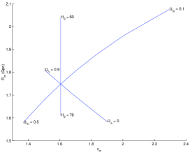
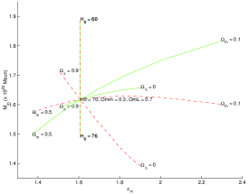
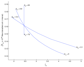
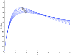
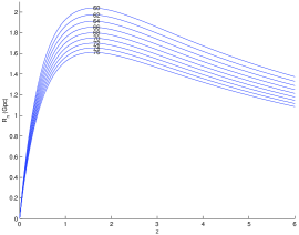
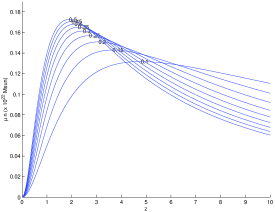
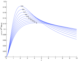
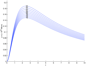
The dependence of $\hat{R}_{m}$, $M_{m}$, ${\cal M}_{m}$ and $\widetilde{\mu n}$ on $H_{0}$, $\Omega_{\Lambda}$ and $\Omega_{m}$ is shown in fig 1, and for reference the $\hat{R}(z)$ and $\mu n(z)$ curves for a range of values of these parameters are given in the appendix.

Figure 1: (a) The dependence of $\hat{R}_{m}$ and $z_{m}$ on the RW parameters; (b) the dependence of $M_{m}$ (solid lines) and ${\cal M}_{m}$ (dashed lines) on the RW parameters. (c) the dependence of $\widetilde{\mu n}_{m}$ and $\tilde{z}_{m}$ on the RW parameters.

V Discussion

The properties outlined in section III below eq (15) make the maximum in $\hat{R}$ a very significant feature of a cosmological model, both theoretically and observationally.

Both $\hat{R}_{m}$ and $z_{m}$ may be measured, and calculating $M_{m}$ from (15) requires only the value of $\Lambda$, and is independent of the details of the cosmology, or even whether large-scale homogeneity exists. Note also that $M_{m}$ is not very sensitive to uncertainties in $\Omega_{\Lambda}$; for a given measured $R_{m}$, an increase from $0$ to $0.7$ decreases the calculated $M_{m}$ by $12$%.

Current galaxy redshift surveys only extend to $z=0.3$, while quasar redshift surveys extend to $z=6$. However the data is not complete enough, and the quasar population too diverse to be useful. The next generation of galaxy surveys will extend past the redshift of the maximum, and recent supernova observations StroEtAl04 are already approaching it. The $\hat{R}$-$z$ plot may be obtained from direct measurements of redshifts and angular diameters, or derived from $m$-$z$ measurements. While the former would be ideal, the latter is acceptable, since the reciprocity theorem is very general. Of course, knowledge (or assumptions) about true diameters and absolute luminosities of sources, and their $z$ evolution, is essential, and at large $z$ this is a significant uncertainty.

While locating $\hat{R}_{m}$ reliably requires a good sample of data points in a range near $z_{m}$, determination of $n(z)$ is not so easy, since one must be sure of detecting or reliably estimating all masses. Nevertheless, a sufficiently deep, complete survey should provide an indication of $\widetilde{\mu n}_{m}$ and $\tilde{z}_{m}$.

An issue for future consideration is the effect of inhomogeneities on the uncertainty in $\hat{R}_{m}$ and $z_{m}$ determinations. For example MuBaHeEl98 showed inhomogeneity can cause loops in the $\hat{R}$-$z$ curve near the maximum.

The mass-to-light ratio is difficult to determine outside gravitationally bound systems, and direct estimates of (gravitational) mass from galaxy and cluster dynamics, and from gravitational lensing only extend up to cluster or supercluster size, whereas the determination of $M_{m}$ reaches several orders of magnitude larger.

The possibility of determining the metric of the cosmos from observations of redshifts, luminosities (or angular diameters) and the number density of sources, combined with the evolution of absolute luminosities, true diameters, and mass per source, was considered in ObsCosmol ; MuHeEl97 ; Hel01 . A project to begin implementing this is now underway LuHel05 . The cosmic mass $M_{m}$ provides an important cross-check on the summed mass at that radius. In fact the theorem of MuHeEl97 — that, given any reasonable set of observations and any reasonable source evolutions functions, an LT model can be found that fits them — needs to be qualified, as the combination of observations and evolution functions must mesh correctly close to $\hat{R}_{m}$.

Within the dust-$\Lambda$-RW model, it is noteworthy that the maximum is where the $\hat{R}(z)$ curve is most sensitive to variations in $\Omega_{\Lambda}$ and $H_{0}$, and nearly so for $\Omega_{m}$, and that variations in these 3 parameters move the $(z_{m},\,\hat{R}_{m})$ and $(\widetilde{\mu n}_{m},\,\tilde{z}_{m})$, loci in very different directions. Thus a determination of $\hat{R}_{m}$ & $z_{m}$ would provide rather generic limits on $H_{0}$, $\Omega_{m}$ and $\Omega_{\Lambda}$, and combined with the initial slope of the $\hat{R}$-$z$ graph, or with measurements of $\widetilde{\mu n}_{m}$ and $\tilde{z}_{m}$, would fix all three values. Determining $\hat{R}_{m}$ and $z_{m}$ to within 10% would by itself provide confirmation (or otherwise) of current parameter estimations, while 5% accuracy would put new constraints on the possible values.

The problem of averaging in GR means that identifying the RW model that best fits the observations is not a well-defined execise. Therefore measurments of bulk effects are particularly important, and since $R_{m}$, unlike any other point on the pnc, gives the total mass on that scale, the $R_{m}$ and $z_{m}$ values provide a natural definition of the best fit RW model.

Although particular models always have a $\hat{R}$-$M$ relation, such as (19) & (20) would give for RW models, this relation is very model dependent, whereas $M_{m}$ is not. It is more general even than the LT model, as any cosmology will have a locus where the past null cone crosses the apparent horizon, and an associated mass is naturally defined there.

VI Conclusion

In summary, the maximum in the diameter distance is the only point on the past null cone that corresponds to a model independent mass, thus allowing direct measurement of a characteristic cosmic mass on gigaparsec scales. Therefore it also provides a very large-scale check on the mass to light ratio, as well as a reference point for determining geometry from observations. Since it is a point on the apparent horizon, a measurement of this maximum may actually be the first detection of a relativistic horizon.

For RW models, the region near the maximum is where $R(z)$ is most sensitive to the values of the RW parameters.

We advocate that, with the next generation of surveys, direct measurements of angular sizes and hence diameter distances be compiled and calculated independently of luminosity distances, and that, apart from fitting a Friedmann-Lemaître-Robertson-Walker (FLRW) model to the available data, a separate determination of $\hat{R}_{m}$ be done with a limited data set near $z_{m}$, thus giving a model independent value for $M_{m}$.

Figure 2: The $\hat{R}(z)$ curves for a range of RW parameters: (a) different $\Omega_{m}$ values ($H_{0}=70$, $\Omega_{\Lambda}=0.7$), (b) $\Omega_{\Lambda}$ values ($H_{0}=70$, $\Omega_{m}=0.3$), (c) $H_{0}$ values ($\Omega_{m}=0.3$, $\Omega_{\Lambda}=0.7$).

Figure 3: The $\mu n(z)$ curves for a range of RW parameters (note that the $z$ scale is different from that of fig. (2): (a) various $\Omega_{m}$ values ($H_{0}=70$, $\Omega_{\Lambda}=0.7$), (b) $\Omega_{\Lambda}$ values ($H_{0}=70$, $\Omega_{m}=0.3$), (c) $H_{0}$ values ($\Omega_{m}=0.3$, $\Omega_{\Lambda}=0.7$).

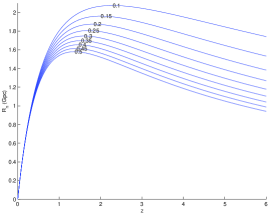
Appendix A Specialising the LT equations to RW

The dust-$\Lambda$-RW model, in its most common coordinate system, is obtained if we put

$$M=M_{0}r^{3}~{},~{}~{}~{}~{}2E=-kr^{2}~{},~{}~{}~{}~{}t_{B}=0~{},$$ (19)

from which we have

$$R=rS(t)~{},~{}~{}~{}~{}~{}\dot{S}^{2}=2M_{0}/S-k+\Lambda S^{2}/3~{},$$ (20)

$$H_{0}=\dot{S}_{0}/S_{0}~{},~{}~{}~{}\kappa\rho=6M_{0}/S^{3}~{},~{}~{}~{}\kappa\rho_{0}=6M_{0}/S_{0}^{3}~{},$$ (21)

where $S$ is the scale factor. Given $H_{0}$, $\Omega_{\Lambda}$ and $\Omega_{m}$, then

$$t_{0} =2/3H_{0}~{},~{}~{}~{}~{}\kappa\rho_{0}=3\Omega_{m}H_{0}^{2}~{},~{}~{}~{}~{}\Lambda=3H_{0}^{2}\Omega_{\Lambda}~{},$$ (22)

$$\Omega_{k} =1-\Omega_{\Lambda}-\Omega_{m}~{},~{}~{}~{}~{}k=-{\rm sign}(\Omega_{k})~{},$$ (23)

$$S_{0} =\left\{\begin{array}[]{ll}\text{arbitrary}&~{}\mbox{if}~{}~{}k=0~{},\\ \frac{1}{H_{0}}\sqrt{\frac{-k}{\Omega_{k}}}&~{}\mbox{if}~{}~{}k\neq 0~{},\end{array}\right.$$ (26)

$$M_{0} =\Omega_{m}H_{0}^{2}S_{0}^{3}/2~{},$$ (27)

where $\Omega_{m}$ is the baryonic plus dark matter fraction. The integrated density equation is

$${\cal M} =\frac{3M_{0}k}{2}\Bigg{(}\frac{\sin^{-1}(\sqrt{k}\;r)}{\sqrt{k}\;}-r\sqrt{1-kr^{2}}\;\Bigg{)}$$ (28)

so for nearly flat models, where $r<<1$,

$$({\cal M}-M)/M\approx 0.3kr^{2}$$ (29)

The pnc and AH equations (5), (8), (9), (15) & (18), using $S_{m}=S(\hat{t}(r_{m}))$, become

$$\hat{t}^{\prime}=\frac{-S}{\sqrt{1-kr^{2}\;}} ~{},$$ (30)

$$\frac{{\rm d}{R_{n}}}{{\rm d}{z}}=\left[\frac{\sqrt{1-kr^{2}}\;-r\dot{S}}{H(1+z)}\right]_{n} ~{},~{}~{}~{}~{}\frac{{\rm d}{R_{n}}}{{\rm d}{z}}\Bigg{|}_{z=0}=\frac{1}{H_{0}}~{},$$ (31)

$$\Lambda r_{m}^{3}\hat{S}_{m}^{3}-3r_{m}\hat{S}_{m} +6M_{0}r_{m}^{3}=0~{},$$ (32)

$$\frac{6M_{0}}{\kappa\dot{S}^{3}(1+z)^{2}}\Big{(}2r\sqrt{1-kr^{2}}\;\dot{S} +r^{2}(S\ddot{S}-\dot{S}^{2})\Big{)}=0$$ (33)

Figs 2 and 3, show $\hat{R}(z)$ and $\mu n(z)$ for a range of $H_{0}$, $\Omega_{\Lambda}$ and $\Omega_{m}$ values. The primary interest is on how these parameters affect the maxima.

References

- (1) http://www.sdss.org/
- (2) http://www.aao.gov.au/2df/
- (3) F. Hoyle, “Cosmological Tests of Gravitational Theories” in Proc. Enrico Fermi School of Physics, Course XX, Varenna, “Evidence for Gravitational Theories”, Ed. C. Moller (Academic Press, New York) (1961), p 141-174. This is apparently the first article to explicitly state the angular diameter corresponding to a fixed physical diameter has a minimum as redshift increases.
- (4) W.E. McCrea “Observable Relations in Relativistic Cosmology”, Zeits. Astrophys., 9, 290-314 (1934). Although the paper doesn’t state the diameter distance has a maximum, equation (55) is the standard result for the diameter distance in an Einstein-de Sitter model.
- (5) G. Lemaître, Ann. Soc. Sci. Bruxelles A53, 51 (1933); reprinted in Gen. Rel. Grav. 29, 641 (1997).
- (6) R. C. Tolman, Proc. Nat. Acad. Sci. USA 20, 169 (1934); reprinted in Gen. Rel. Grav. 29, 935 (1997).
- (7) C Hellaby, K. Lake, Astrophys. J. 290, 381 (1985) [+ erratum: Astrophys. J. 300, 461 (1985)].
- (8) A. Krasiński, “Inhomogeneous Cosmological Models”, Cambridge U P (1997), ISBN 0 521 48180 5.
- (9) N. Mustapha, C. Hellaby and G.F.R. Ellis Mon. Not. Roy. Astro. Soc. 292, 817-30, (1997).
- (10) N. Mustapha, B.A.C.C. Bassett, C. Hellaby and G.F.R. Ellis Class. Q. Grav. 15, 2363-79, (1998).
- (11) C. Hellaby Astron. Astrophys. 372, 357-363 (2001).
- (12) C. Hellaby, Class. Q. Grav. 4, 635 (1987).
- (13) A. Krasiński and C. Hellaby, Phys. Rev. D 69, 043502 (2004).
- (14) G.F.R. Ellis and G. Tivon, The Observatory 105, 189 (1985).
- (15) L.-G. Strolger Et Al, Astrophys. J. 613, 200-223 (2004).
- (16) J. Kristian and R.K. Sachs (1966) Astrophys. J. 143, 379-99. G.F.R. Ellis, S.D. Nel, R. Maartens, W.R. Stoeger, & A.P. Whitman (1985) Phys. Reports 124, 315-417. W.R. Stoeger, S.D. Nel, R. Maartens & G.F.R. Ellis (1992), Class. Q. Grav., 9, 493-507. W.R. Stoeger, G.F.R. Ellis & S.D. Nel (1992a), Class. Q. Grav., 9, 509-26. W.R. Stoeger, S.D. Nel & G.F.R. Ellis (1992b), Class. Q. Grav., 9, 1711-23. W.R. Stoeger, S.D. Nel & G.F.R. Ellis (1992c), Class. Q. Grav., 9, 1725-51. R. Maartens, D.R. Matravers (1994) Class. Q. Grav. 11, 2693-704. M.E. Araújo & W.R. Stoeger (1999) Phys. Rev. D, 60, 104020, 1-7; plus Errata in (2001) Phys. Rev. D, 64, 049901, 1. M.N. Celerier, Astron. Astrophys. 353 63-71 (2000). M.E. Araújo, R.C. Arcuri, J.L. Bedran, L.R. de Freitas, & W.R. Stoeger (2001) Astrophys. J. 549, 716-20. M.E. Araújo, S.R.M.M. Roveda & W.R. Stoeger (2001) Astrophys. J. 560, 7-14. M.B. Ribeiro & W.R. Stoeger, (2003) Astrophys. J. 592, 1-16.
- (17) H.-C. Lu, C. Hellaby, in preparation (2005).