The white dwarf luminosity function. I. Statistical errors and alternatives

Abstract

The white dwarf luminosity function is an important tool for the study of the solar neighborhood, since it allows the determination of the age of the Galactic disk. Over the years, several methods have been proposed to compute galaxy luminosity functions, from the most simple ones — counting sample objects inside a given volume — to very sophisticated ones — like the C^- method, the STY method or the Choloniewski method, among others. However, only the $1/\mathcal{V}_{\rm max}$ method is usually employed in computing the white dwarf luminosity function and other methods have not been applied so far to the observational sample of spectroscopically identified white dwarfs — in sharp contrast with the situation when galaxy luminosity functions are derived from a large variety of samples. Moreover, the statistical significance of the white dwarf luminosity function has also received little attention and a thorough study still remains to be done. In this paper we study, using a controlled synthetic sample of white dwarfs generated using a Monte Carlo simulator, which is the statistical significance of the white dwarf luminosity function and which are the expected biases. We also present a comparison between different estimators for computing the white dwarf luminosity function. We find that for sample sizes large enough the $1/\mathcal{V}_{\rm max}$ method provides a reliable characterization of the white dwarf luminosity function, provided that the input sample is selected carefully. Particularly, the $1/\mathcal{V}_{\rm max}$ method recovers well the position of the cut–off of the white dwarf luminosity function. However, this method turns out to be less robust than the Choloniewski method when the possible incompletenesses of the sample are taken into account. We also find that the Choloniewski method performs better than the $1/\mathcal{V}_{\rm max}$ method in estimating the overall density of white dwarfs, but misses the exact location of the cut–off of the white dwarf luminosity function.

1 Introduction

The white dwarf luminosity function is perhaps one of the most useful tools for deriving important properties of the solar neighborhood. In particular, but not only, the disk white dwarf luminosity function carries valuable information about the age of the Galaxy (Winget et al. 1987; García–Berro et al. 1988; Hernanz et al. 1994; Richer et al. 2000) and of the stellar formation rate (Noh & Scalo 1990; Díaz–Pinto et al. 1994; Isern et al. 1995; Isern et al. 2001). Additionally, the luminosity function of white dwarfs provides an independent test of the theory of dense plasmas (Segretain et al. 1994; Isern et al. 1997). Finally, the white dwarf luminosity function directly measures the current death rate of low– and intermediate–mass stars in the local disk. Consequently, a reliable determination of the observational white dwarf luminosity function is of the maximum interest.

Previous observational efforts, like the Palomar Green Survey (Green et al. 1986) have provided us with an invaluable wealth of good quality data. Moreover, ongoing projects like the Sloan Digital Sky Survey (York et al. 2000; Stoughton et al. 2002; Abazajian et al. 2003, 2004), the 2 Micron All Sky Survey (Skrutskie et al. 1997; Cutri et al. 2003), the SuperCosmos Sky Survey (Hambly et al. 2001a; Hambly, et al. 2001b; Hambly, Irwin & MacGillivray 2001), the 2dF QSO Redshift Survey (Vennes et al. 2002), the SPY project (Pauli et al. 2003), and others will undoubtely increase the sample of spectroscopically identified white dwarfs with reliable determinations of parallaxes and proper motions, which are essential for an accurate determination of the white dwarf luminosity function. Last but not least, future space missions like Gaia (Perryman et al. 2001) will increase the sample of known white dwarfs with very accurate astrometric determinations even further (Torres et al. 2005), thus allowing a precise and reliable determination of the properties of the disk white dwarf population.

Over the years, several methods have been used to determine luminosity functions for all sort of objects, ranging from main sequence stars to galaxies. These include the most simple ones (counting stars inside a given volume) to very sophisticated ones — like the C^- method (Lynden-Bell 1971), the STY method (Sandage et al. 1979) and the Choloniewski method (Choloniewski 1986). In spite of the variety of methods currently used to estimate galaxy luminosity functions, the $1/\mathcal{V}_{\rm max}$ method (Schmidt 1968) is the most commonly used method for estimating white dwarf luminosity functions, though, to the best of our knowledge, nobody has yet assesed in depth its statistical reliability for such a purpose. More specifically, up to now only two works have studied how good the $1/\mathcal{V}_{\rm max}$ method performs in estimating the white dwarf luminosity function. In particular, Wood & Oswalt (1998) demonstrated by using a Monte Carlo simulator that the $1/\mathcal{V}_{\rm max}$ method for proper–motion selected samples is a good density estimator, although it shows important statistical fluctuations when estimating the slope of the bright end of the white dwarf luminosity function. Later on, García–Berro et al. (1999), using another Monte Carlo simulator, corroborated the previous study and, moreover, showed that the standard procedure used by the $1/\mathcal{V}_{\rm max}$ method to asign error bars severely understimates the size of the real error bars for a typical sample of 200 objects. Additionally these last authors also showed that there was a bias in the derived ages of the solar neighborhood, consequence of the binning procedure. However, the most apparent conclusion of both papers is that, in general, selection effects or, simply, the inherent characteristics of the sample under consideration have a strong effect on the shape of the estimated white dwarf luminosity function, despite using an unbiased estimator, like the $1/\mathcal{V}_{\rm max}$ method.

In this paper we assess the statistical significance of the observational white dwarf luminosity function. For such a purpose we will use a controlled synthetic sample of white dwarfs generated with our Monte Carlo simulator. We discuss in depth which are the typical biases introduced by the procedures used to select the sample. This includes both the bias in retrieving the correct slope for the monotonically increasing branch of the white dwarf luminosity function and, most importantly, the bias obtained when retrieving the precise location of the observed cut–off. This last point is of the maximum interest, since the observed drop–off of the white dwarf luminosity is currently one of the best estimators used to date the local neighborhood. We also present an independent estimate of the size of the error bars. Finally we discuss the advantages and shortcomings of the several methods that can be used to obtain the observational white dwarf luminosity function and we present a set of recommendations. The reader should take into account that in the present paper we only discuss the sampling biases and do not take into account the measurement errors. Clearly, the effects of the measurement errors will affect the sampling biases and viceversa. Moreover, the effects of the measurement errors could be as important as the sampling biases, although this remains still to be studied. Such an study is under preparation and will be published elsewhere. The paper is organized as follows. In section 2 we describe the different estimators most commonly used today for obtaining luminosity functions. Section 3 is devoted to describe the Monte Carlo simulations used to compare the different methods previously described in §2, whereas in Section 4 we apply the different estimators to our Monte Carlo samples. Finally in Section 5 we summarize our major findings and we draw our conclusions.

2 The most commonly used luminosity function estimators

2.1 Schmidt’s estimator for proper motion and magnitude selected samples

This method, also known as the $1/\mathcal{V}_{\rm max}$ method, was first introduced by Schmidt (1968) in the studies of the quasar population. Later on Schmidt (1975) extended it to proper motion selected samples and Felten (1976) made a generalization of the method introducing the dependence on the direction of the sample. This turns out to be useful when studying stellar samples because the scale height of the Galactic disk introduces some biases.

Consider a sample of stars having a lower proper motion limit $\mu_{\rm l}$ and faint apparent magnitude limit $m_{\rm f}$, the maximum distance for which an object can contribute to the sample is:

$$r_{\max}=\min\left[\pi^{-1}(\mu/\mu_{\rm l});\pi^{-1}10^{0.2(m_{\rm f}-m)}\right]$$ (1)

where $\pi$ is the stellar parallax, $\mu$ is the proper motion, and $m$ the apparent magnitude. If the sample is only complete to a certain upper proper–motion limit $\mu_{\rm u}$ and to a bright magnitude limit $m_{\rm b}$, then there is also a minimum distance for which an object contributes to the luminosity function:

$$r_{\min}=\max\left[\pi^{-1}(\mu/\mu_{\rm u});\pi^{-1}10^{0.2(m_{\rm b}-m)}\right]$$ (2)

Additionally, if the sample only covers a fraction of the sky, $\beta$, then the maximum volume in which a star can contribute is:

$$\mathcal{V}_{\max}=\frac{4\pi}{3}\beta(r_{\max}^{3}-r_{\min}^{3})$$ (3)

The luminosity function, $\varphi_{M}$, is then built by binning the sample in $i\in(1,N)$ magnitude bins and performing a weighted sum over the objects in each magnitude bin, $N_{i}$. The weight with which every object contributes to the sum depends on the maximum volume in which it could be detected given its apparent magnitude and proper motion:

$$\varphi(M_{i})={\displaystyle\sum\limits_{j=1}^{N_{i}}}\frac{1}{\mathcal{V}^{j}_{\max}}$$ (4)

Though this estimator is based on heuristic appreciations about how a good estimator should be, it has been shown that it is unbiased (Felten 1976). However, the fact that the estimator is unbiased does not guarantee a good estimate of the luminosity function if the input data is not properly selected. More specifically, the input sample should be complete and, additionally, Takeuchi et al. (2000) have pointed out that the $1/\mathcal{V}_{\rm max}$ method for magnitude selected samples is seriously affected when the input data — even if complete — is clustered or, more generally speaking, when the input data are not homogenously scattered. This, in turn, affects the derived shape of the luminosity function. Consequently, the $1/\mathcal{V}_{\rm max}$ method should only be used when homogeneity and completitude of the sample under consideration are guaranteed. This, of course, is not an easy task, and for most of the observational samples is an “a priori” assumption.

2.2 Maximum Likelihood estimators based on the probability of selection

Maximum likelihood estimators are based on the probability of selecting a given object in a sample and have been shown to be insensitive to sample inhomogenities. Moreover, by definition, these estimators are unbiased and have minimum variance for large samples. Two variants have been already developed. The first one is a parametric estimator (Sandage et al. 1979), hereafter the STY estimator, whereas the corresponding non–parametric version (Efstathiou et al. 1988) is called the StepWise Maximum Likelihood estimator (SWML). Both estimators are designed for magnitude selected samples and their performances when evaluating galaxy luminosity functions have been thoroughly tested using detailed Monte Carlo simulations (Willmer 1997; Takeuchi et al. 2000).

Following Luri et al. (1996) we define the likelihood function, $\mathcal{L}$, as the product of the probability distributions of the variables of interest, under the assumption that all of them are statistically independent:

$$\mathcal{L}(\theta)={\prod\limits_{k=1}^{n_{x}}}\mathcal{D}(x_{k}|\theta)$$ (5)

where $x$ is a random variable with probability density $\mathcal{D}(x_{k}|\theta)$ depending on a set of unknown parameters $\theta=(\theta_{1},\theta_{2},\ldots,\theta_{n})$ and realizations $(x_{1},\ldots,x_{n_{x}})$. The value of $\theta$ that maximizes this function is the maximum likelihood estimator, $\theta_{\rm ML}$, of the parameters.

Observational selection may be modelled by introducing a new probability density, $\mathcal{M}(x_{k}|\theta)$, with the help of a normalization constant, $\mathcal{C}_{M}^{-1}$, which depends upon the maximization variables, and of a selection function, $\mathcal{S}(x_{k})$:

$$\mathcal{M}(x_{k}|\theta)=\mathcal{C}_{M}^{-1}\mathcal{D}(x_{k}|\theta)\mathcal{S}(x_{k})$$ (6)

A typical example of such a selection function is that obtained for the case of a sample which is complete up to a certain limiting apparent magnitude, $m_{\rm lim}$. In this case the selection function is simply a Heaviside function, $\mathcal{S}(m_{k})=\Theta(m_{k}-m_{\lim})$. Writing down the probability distribution as the product of the densities of the variables of interest in our sample — absolute magnitude, $M$, parallax, $\pi$, and tangential velocity, $v_{\rm tan}$ — we get the structure of the STY and SWML estimators for magnitude selected samples:

$$\mathcal{M}(M_{k}|\theta)\propto\frac{\varphi(M_{k}|\theta)}{\int\varphi(M|\theta)dM}$$ (7)

$$\mathcal{L}(\theta)={\prod\limits_{k=1}^{n_{x}}}\mathcal{M}(M_{k}|\theta)$$ (8)

It becomes obvious from the definition of likelihood that the statistical independence of the variables makes the maximization process insensitive to the distribution of velocities and to the parallax probability density. Note, however, that for the case in which we have a mixture of populations (thin and thick disk and halo, for instance) the velocities and the absolute magnitude are no longer independent variables. The SWML method is then obtained by adopting for $\varphi$ as a stepwise function:

$$\varphi(M)=\sum_{i=1}^{N}\hat{\varphi}_{i}W(M_{i}-M)$$ (9)

where the window function $W(M_{i}-M),$ is defined by:

$$W(M_{i}-M)\equiv\left\{\begin{array}[l]{cl}1&{\rm if\ \ }M_{i}-\frac{\Delta M}{2}\leq M\leq M_{i}+\frac{\Delta M}{2}\\ 0&{\rm otherwise}\end{array}\right.$$ (10)

and $\hat{\varphi}_{i}$ yields the luminosity function of the corresponding magnitude bin. On the other hand, the STY estimator is obtained by adopting for $\varphi$ a parametric function as, for example, a Schechter function (Schechter 1976). For the case under study we have modified the Schechter function to adapt it to the characteristics of our problem:

$$\varphi(M)\propto 10^{0.4(M^{\star}-M)(A+1)}\exp(-10^{1.6(M^{\star}-M)(A+1)})$$ (11)

where the parameters $A$ and $M^{\star}$ are related with the slope and with the position of the cut–off of the white dwarf luminosity function, respectively. It is worth noticing that this is a good characterization of the luminosity function when the cut–off is sharp. The real white dwarf luminosity function does not show such a sharp cut–off but, instead, a tail extending to fainter magnitudes is observationally found (Oswalt et al. 1996). This is the reason why this method cannot be applied to real samples but to simplified synthetic samples in which this tail is not present (see §3 below). In both cases, the likelihood can be maximized using standard methods. The main drawback of these methods is that they can obtain the shape of the luminosity function but do not provide the normalization factor.

2.3 Maximum likelihood estimators based on poissonian statistics

As an alternative to the estimators shown in the previous sections, there exist other maximum likelihood estimators that build the likelihood using a different approach. Taking as a premise that local distribution of objects in some pair of variables of the sample has a poissonian distribution, it is possible to define a likelihood as a function of the parameter space. The first of such methods, the C^- method, was proposed by Lynden-Bell (1971) and was later improved by Choloniewski (1986). The Choloniewski method uses simple data to define a probabilistic model and then a new likelihood, by dividing the parameter space (magnitude and parallax in our case) in cells and assuming poissonian statistics for each cell. This method allows to estimate both the shape of the luminosity function and the total density of objects simultaneously.

We consider a sample with a total number of $N_{\rm obj}$ objects having absolute magnitudes $M_{i}$ and parallaxes $\pi_{i}$, with $i=1,\ldots,N_{\rm obj}$. The method is restricted to a solid angle $\Omega=4\pi\beta$. Moreover, the absolute magnitude is assumed to fall within $M\in[M_{0},M_{A}]$ and the parallax also obeys $\pi\in[\pi_{0},\pi_{B}]$. This defines a volume:

$$V_{t}=\frac{\Omega}{3}(r_{B}^{3}-r_{0}^{3})$$ (12)

where $r_{0}=1/\pi_{0}$ and $r_{B}=1/\pi_{b}$. Consequently, the number density can be written as

$$n=\frac{N_{c}}{V_{t}}$$ (13)

and the luminosity function and spatial density of the sample are, respectively:

$$\int^{M_{A}}_{M_{0}}\varphi(M)\,dM=n$$ (14)

$$\int V_{t}\varrho(x,y,z)\,dxdydz=N_{\rm obj}$$ (15)

where $\varrho$ is the spatial density of the sample of objects. The key point of the method is to assume that the number of objects in every interval $dM\,dxdydz$ is given by a poissonian random process and that, consequently, the probability of finding $k$ objects in each box can be modelled using the following expression:

$$P_{k}=\exp(-\lambda)\frac{\lambda^{k}}{k!}$$ (16)

Figure 1: Distance versus absolute magnitude for a sample population of white dwarfs. Also shown are the limiting magnitude and the parameter space, $S$, adopted for the calculation of the luminosity function using the Choloniewski method. See text for details.

If, furthermore, the distribution in absolute magnitude and the spatial density distribution are assumed to be independent — which may not be the case if different kinematic populations are present in the sample — we have:

$$\lambda=\frac{1}{n}\varphi(M)\varrho(x,y,z)\,dM\,dxdydz$$ (17)

In order to build the likelihood, the previous expressions are discretized by considering the distribution of objects in the $(M,\pi)$ plane, and binning it into square boxes (see figure 1). We set $\Delta M=\Delta\pi=\Delta$ and $M_{i}=M_{0}+i\Delta$ and $\pi_{j}=\pi_{0}+j\Delta$ with $j=0,\ldots,A$, and $i=0,\ldots,B$. We denote the number of objects that can be found in the box $(i,j)$ as $N_{ij}$ and so the binned probability can be written as:

$$P_{N_{ij}}=\exp(-\lambda_{ij})\frac{\lambda_{ij}^{N_{ij}}}{N_{ij}!},$$ (18)

with:

$$\lambda_{ij}=\frac{1}{n}\hat{\varphi}_{i}\hat{\varrho}_{j}\Delta\frac{\Omega}{3}(r_{j}^{3}-r_{j-1}^{3})$$ (19)

being $\hat{\varphi}_{i}$ closely related to the luminosity function in the given magnitude interval through the expression:

$$\hat{\varphi}_{i}=\int^{M_{i-1}}_{M_{i}}\varphi(M)dM\times\left[\int^{M_{i-1}}_{M_{i}}dM\right]^{-1},$$ (20)

whereas the spatial density is given by:

$$\hat{\varrho}_{j}=\int_{r_{j-1}}^{r_{j}}\int_{\Omega}\varrho(x,y,z)r^{2}\,dr\,d\Omega\times\left[\int_{r_{j-1}}^{r_{j}}\int_{\Omega}r^{2}\,dr\,d\Omega\right]^{-1}$$ (21)

Finally, we mention that the Choloniewski likelihood must be computed considering the selection effects. As the sample only provides information for apparent magnitudes up to a limiting magnitude $m\leq m_{\rm lim}$, the value of the number of objects in each box is only known for the region below the selection line. Thus, we have

$$\mathcal{L}(\theta)={\prod_{i=1}^{A}\prod_{j=1}^{B}}_{i,j\in S}\exp(-\lambda_{ij})\frac{\lambda_{ij}^{N_{ij}}}{N_{ij}}$$ (22)

where $S$ stands for grid in the parameter space (see figure 1). This likelihood can, again, be maximized using standard methods.

3 The Monte Carlo Simulations

Our Monte Carlo simulator has been thouroughly described in previous papers (García–Berro et al. 1997; García–Berro et al. 2004) so here we will only summarize the most important inputs. We have used a pseudo–random number generator algorithm (James 1990) which provides a uniform probability density within the interval $(0,1)$ and ensures a repetition period of $\ga 10^{18}$, which is virtually infinite for practical simulations. When gaussian probability functions are needed we have used the Box-Muller algorithm (Press et al. 1986).

Since we want to test the behaviour of the proposed estimators previously discussed in §2 under different assumptions for the underlying white dwarf population we have analyzed a series of different scenarios with controlled stellar parameters. In a first set of simulations we have adopted the most simple prescriptions for the stellar evolutionary inputs. Specifically, we have adopted the most simple cooling law (Mestel 1952). Consequently, emission of neutrinos was not considered. Crystallization and phase separation were also disregarded. Additionally, for all white dwarfs we adopt the same cooling sequence, namely that of a typical $0.6\,M_{\sun}$ white dwarf, independently of its respective mass. Thus, the effects of the mass spectrum of white dwarfs are also completely disregarded. The initial–to–final mass relationship for white dwarfs and the main sequence lifetime of their progenitors adopted here were the analytical expressions of Iben & Laughlin (1989). Finally, no bolometric corrections were used. Also a very simple galactic model has been used. In particular, a standard initial mass function (Scalo 1998) and a constant volumetric star formation rate were adopted. The velocities have been drawn from normal laws taking into account the differential rotation of the disk and the peculiar velocity of the Sun with respect to the local standard of rest. Since the effect of the spatial distribution of the white dwarf population can be important, we have performed two kinds of simulations: in the first one a uniform distribution was used, whereas for the second one a constant scale height of 300 pc was assumed.

Table 1: Summary of models

Model	Cooling	$r_{\rm max}$	$z$-distribution
	sequences
1	Mestel (1952)	250 pc	Uniform
2	Mestel (1952)	1800 pc	Uniform
3	Mestel (1952)	1800 pc	$h=300$ pc
4	Salaris et al. (2000)	1800 pc	Time-dependent $h$

In a second stage a set of more realistic model simulations has also been performed. For this second set of simulations the cooling sequences of Salaris et al. (2000) which incorporate the most accurate physical inputs for the stellar interior (including neutrinos, crystallization and phase separation) and reproduce the blue turn at low luminosities (Hansen 1998) have been used. Also, these cooling sequences encompass the full range of interest of white dwarf masses, so a complete coverage of the effects of the mass spectrum of the white dwarf population was taken into account. Besides, the spatial density distribution is obtained from a scale height law (Isern et al. 1995) which varies with time and is related to the velocity distributions.

All the simulations presented here are the average of an ensemble of 400 independent realizations. In all the cases but in the first one the white dwarf population was modelled up to distances of $r_{\rm max}=1800$ pc, in order to avoid the effects of the border and were normalized to the local space density of white dwarfs within 250 pc, $n=0.5\times 10^{-3}$ pc^-3 for $M_{V}<12.75^{\rm mag}$ (Liebert, Bergeron & Holberg 2005). For model 1 we adopted $r_{\rm max}=250$ pc in order to test the effects of a distance-limited sample. Table 1 summarizes the main characteristics of each simulation.

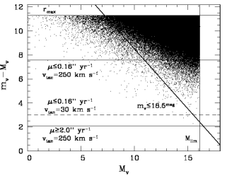
Figure 2: Distance modulus versus absolute magnitude for a whole population of white dwarfs within a 1800 pc in a uniform distribution. Also shown are the selection criteria in proper motion and apparent magnitude. See text for details.

4 Results

4.1 The $1/\cal{V}_{\rm max}$ method: slope, cut–off and binning

We start discussing model 1. Since the final goal is to compute the white dwarf luminosity function a set of restrictions is needed for selecting a subset of white dwarfs which, in principle, should be representative of the whole white dwarf population. We have chosen the following criteria for selecting the final sample: $m_{\rm V}\leq 18.5^{\rm mag}$ and $\mu\geq 0.16^{\prime\prime}\;{\rm yr}^{-1}$ as it was done in Oswalt et al. (1996). We do not consider white dwarfs with very small parallaxes $(\pi\leq 0.005^{\prime\prime})$, since these are unlikely to belong to a realistic observational sample. Additionally, all white dwarfs brighter than $M_{\rm V}\leq 13^{\rm mag}$ are included in the sample, regardless of their proper motions, since the luminosity function of hot white dwarfs has been obtained from a catalog of spectroscopically identified white dwarfs (Green 1980; Fleming et al. 1986) which is assumed to be complete (Liebert, Bergeron & Holberg 2005). Moreover, all white dwarfs with tangential velocities larger than 250 km s^-1 were discarded (Liebert et al. 1989) since these would be probably classified as halo members. With all these inputs the white dwarf luminosity function should have a constant slope and a very sharp cut–off, which depends on the adopted age of the disk. Given the cooling law adopted here the slope turns out to be 5/7 and, moreover, considering that the cut–off of the observational white dwarf luminosity function is located at $\log(L/L_{\sun})\simeq-4.6$ (Liebert et al. 1988) the adopted age of the disk turns out to be 13 Gyr.

Figure 3: a) A sample of 20 realizations of the disk white dwarf luminosity function. b) Average and standard deviation of the 400 realizations of the white dwarf luminosity function.

In order to illustrate the effects of the previous restrictions in the final sample, in figure 2 we show the distance modulus as a function of the absolute $V$ magnitude for the whole white dwarf population of a given realization of our Monte Carlo simulations. The upper horizontal line corresponds to the maximum distance to which our synthetic population extends (1800 pc). The vertical line corresponds to the limiting absolute magnitude, $M_{\rm lim}$, which is directly obtained from the adopted age of the disk and the Mestel cooling law used in this set of simulations. The diagonal line corresponds to the limiting magnitude imposed by the selection criteria previously mentioned. On the other hand, there is as well a maximum distance for which a white dwarf could be found within the proper motion limit. In particular, an object should have a tangential velocity smaller than 250 km s^-1 to be considered as a disk white dwarf, otherwise it would be considered a halo member. Note, however, that most of the synthetic white dwarfs above this line have tangential velocities considerably smaller than 250 km s^-1 and, consequently have proper motions smaller than the proper motion cut. We have drawn an horizontal line for this maximum distance ($r=330$ pc) for which a white dwarf could be considered as a disk member. The upper dotted line in this diagram corresponds to the distance for which an otherwise typical white dwarf with $v_{\rm tan}=30$ km s^-1 would be included in the final sample of white dwarfs ($r=65$ pc). Finally, it is worth noticing that the currently available proper motions surveys are not sensitive to large proper motions. A representative upper cut in proper motion could be $\mu_{\rm u}=2^{\prime\prime}$ yr^-1. The solid bottom horizontal line in Fig. 2 represents the corresponding distance for a high velocity white dwarf with $v_{\rm tan}=250$ km s^-1, representative of the halo population. As can be seen in Fig. 2 the effects of the selection criteria are dramatical and only an extremely small percentage of the whole white dwarf population meets the selection criteria and, consequently, are culled for building the white dwarf luminosity function.

Fig. 3a shows 20 independent realizations of the white dwarf luminosity function, computed with the $1/\mathcal{V}_{\rm max}$ method, binned in 2 bins (top panel), 4 bins (middle panel) and 8 bins (bottom panel) per decade. The solid lines correspond to the theoretical expectations previously described. That is, a straight line with constant slope and a very sharp cut–off at the observed position. Each sample typically contains about 300 white dwarfs, the size of the observational sample. We recall that, by construction, our samples are complete. As can be seen, there is a considerable spread about the theoretical expectations and, moreover, the white dwarf luminosity function is underestimated at moderately high luminosities. On the other hand, Fig. 3b shows the average and standard deviation of the 400 realizations of the white dwarf luminosity function. Again it is clearly visible that the $1/\mathcal{V}_{\rm max}$ method considerably underestimates the density of white dwarfs with moderately high luminosities. In fact, the $1/\mathcal{V}_{\rm max}$ method only recovers the right slope for luminosities smaller than $\log(L/L_{\sun})\simeq-2.2$. Moreover, the position of the cut–off also depends on how the data is binned, its position being more accurate for finer binning, and it is always located at larger luminosities, a direct consequence of the binning procedure, as already found by García–Berro et al (1999).

Figure 4: a) Distribution of slopes for the white dwarf luminosity functions of Fig 3. b) Distribution of cut–offs for the white dwarf luminosity functions of Fig. 3.

In order to quantify the previous statements Fig. 4a shows the frequency distribution of slopes for the 400 independent realizations of the white dwarf luminosity function. The vertical solid line corresponds to the theoretical value of the slope of the white dwarf luminosity function (5/7). Obviously all the realizations severely overestimate the slope and, moreover, there is a considerable dispersion. On the other hand, in Fig. 4b the distribution of simulated cut–offs is shown. Clearly, the finer the binning the more accurate is the determination of the cut–off. However, the dispersion is relatively small. That is, this is a systematic bias, which can be accounted for and ultimately corrected.

Another important information that can be readily obtained from our simulations is how to compare the observational procedure to assign error bars — basically assuming poissonian statistics for each bin (Liebert et al. 1988) — with the computed standard deviations, $\Delta\log\varphi_{\rm std}$. To be more specific the contribution of each star to the total error budget in its luminosity bin, $\Delta\log\varphi_{\rm obs}$, is conservatively estimated to be the same amount that contributes to the resulting density; the partial contributions of each star in the bin are squared and then added, the final error is the square root of this value. Table 2 shows the result of such a comparison. As can be seen, we have found that, in general, the standard procedure to assign error bars severely underestimates the observational error bars, especially for the brigthest luminosity bins of the luminosity function. Particularly, for these luminosity bins the error bars are underestimated by a factor of roughly $\approx 10$, whereas for the two (more populated) dimmest luminosity bins the error bar and the inherent statistical deviation are very similar.

Table 2: A comparison of the error bars of the white dwarf luminosity function computed using the $1/\mathcal{V}_{\rm max}$ method, $\Delta\log\varphi_{\rm obs}$, with the standard observational procedure to assign error bars with the intrinsic statistical deviation of the 400 realizations for the white dwarf population of model 1, $\Delta\log\varphi_{\rm std}$. The white dwarf luminosity function has been obtained by binning the synthetic data in four luminosity bins per decade.

$-\log(L/L_{\sun})$	$\Delta\log\varphi_{\rm obs}$	$\Delta\log\varphi_{\rm std}$
1.625	$-7.155$	$-5.796$
1.875	$-7.222$	$-5.535$
2.125	$-7.097$	$-5.207$
2.375	$-5.886$	$-5.016$
2.625	$-5.824$	$-4.838$
2.875	$-6.000$	$-4.689$
3.125	$-5.699$	$-4.405$
3.375	$-5.398$	$-4.291$
3.625	$-5.046$	$-4.165$
3.875	$-5.155$	$-3.925$
4.125	$-4.823$	$-4.064$
4.375	$-4.921$	$-5.063$

4.2 Looking for an alternative: other estimators

Figure 5: a) A comparison of the white dwarf luminosity functions obtained using alternative methods and the $1/\mathcal{V}_{\rm max}$ method. b) Distribution of cut–offs for the different realizations of the white dwarf population using different methods.

As we have shown, the $1/\mathcal{V}_{\rm max}$ method does not provide satisfactory answers with regard to the slope of the white dwarf luminosity function and the position of the cut–off for the white dwarf populations of model 1. Thus, some alternatives must be explored. As previously mentioned, there exist several such alternatives. For the sake of conciseness here we will discuss only two of them: the STY method (Sandage et al. 1979) and the Choloniewski method (Choloniewski 1986). The SWML method (Efstathiou et al. 1988) gives results which are very similar to the STY method and, thus, we will not describe them in detail for the moment. All three methods are maximum likelihood methods and have been consistently used to estimate galaxy luminosity functions. And this is perhaps their main drawback since they have not been devised to correct for the bias in proper motion. This is a characteristic of the current white dwarf samples, and the $1/\mathcal{V}_{\rm max}$ method does correct it. However, as it will be shown below this is not a severe problem, at least for the STY method. We must recall that the STY method provides the shape of the luminosity function but not its normalization (namely, the true density of objects), whereas the Choloniewski method provides both the shape of the luminosity function and the density of objects. The selection criteria used in this set of simulations are exactly the same used previously for deriving the white dwarf luminosity function using the $1/\mathcal{V}_{\rm max}$ method.

Fig. 5a shows a comparison of the results obtained for our model 1 using the different methods discussed here. The bottom panel is the same already shown in the middle panel of Fig. 3b. The middle panel shows the results obtained using the STY method, and as can be seen, the STY method recovers very well the correct slope. Finally, the top panel shows the results obtained using the Choloniewski method. Clearly, this method underestimates the slope at high luminosities. The reason for this is quite clear: the statistics of the brightest luminosity bins are not poissonian. In fact, very few white dwarfs populate these bright luminosity bins (note that the vertical scales in Fig. 3 and 5 are logarithmic). Consequently, the results obtained using the Choloniewski method for the brightest luminosity bins are not correct. However this method turns out to be very useful since we obtain the correct density of white dwarfs. In all three cases the error bars are similar. On the other hand, Fig. 5b shows the position of the cut–off for all three methods. The STY method provides better results than the $1/\mathcal{V}_{\rm max}$ method but, undoubtely, the Choloniewski method performs the best, although with a larger variance than the STY method. Finally, the statistical error bars for all three methods are rather similar, being somehow smaller for the Choloniewski method.

4.3 Extending the sample to larger distances

Figure 6: Same as Fig. 5a for the white dwarf population of model 2.

One possible reason for the systematic bias found when using the $1/\mathcal{V}_{\rm max}$ method to obtain the white dwarf luminosity function could be due to the fact that bright objects can be found at distances considerably larger than 250 pc, the maximum distance within which we have distributed synthetic white dwarfs in model 1. For instance, an object with $\log(L/L_{\sun})=-1.0$ will be within our apparent magnitude selection criterion even if it is located at distances as far as 1800 pc. For this reason we have applied the different luminosity function estimators to a sample with a larger maximum distance, in particular to a sample of synthetic white dwarfs distributed within a sphere of radius 1800 pc (model 2 in Table 1). Since in this sample the effects of the scale height should be important we have carried out an additional simulation in which the synthetic white dwarfs, instead of being distributed according to an uniform density law, have been distributed according to an exponentially decrasing density law. This model will be discussed in section 4.4 below. In both cases the rest of the galactic and stellar evolutionary inputs remain unchanged. Note, however, that in the sample of spectroscopically identified white dwarfs of McCook & Sion (1999) — the primary observational source from which the white dwarf luminosity function is built — the most distant white dwarf with a reliable parallax determination is located at $\sim 250$ pc.

In figure 6 the luminosity functions for the white dwarf population of model 2 are shown for the three estimators previously discussed. The results shown here are the ensemble average and standard deviation of a set of 20 realizations. As can be seen, now the $1/\mathcal{V}_{\rm max}$ estimator correctly matches the theoretical expectations for the slope of the white dwarf luminosity, although with a considerably large variance for the brightest luminosity bins. The reason for this behavior will be discussed below, with the help of figure 7. Also, it is interesting to note that for this set of simulations the STY estimator also yields reasonable results, whereas the Choloniewski estimator largely underestimates the white dwarf density for the luminosity bins near the maximum of the white dwarf luminosity function. Finally, the three estimators obtain the same cut–offs previously obtained for model 1, as it should be expected, given that the population of faint white dwarfs is drawn from distances smaller than 300 pc.

Figure 7: Distance modulus versus magnitude for a typical realization of the white dwarf population of models 1 and 2. The diagonal lines represent the adopted bins of the white dwarf luminosity funcion. The top panel shows the results for a sphere of 1800 pc with a uniform density law (model 2), whereas the bottom panel shows the results for a sphere of 250 pc, also with a uniform density distribution.

In Fig. 7 the distribution of the distance modulus as a function of the magnitude for the synthetic white dwarf populations of models 1 (bottom panel) and 2 (top panel) are shown. We have also represented the diagonal lines corresponding to the adopted bins of the white dwarf luminosity function, from $\log(L/L_{\sun})=-1.0$ (top line) to $-5.0$ (bottom line). The horizontal line corresponds to $r=250$ pc. As can be seen, for model 2 (the sample distributed within 1800 pc) a sizeable number of intrinsically bright white dwarfs (at large distances) meet the selection criteria and, consequently, contribute to the white dwarf luminosity function. In the sample obtained from model 1 these intrinsically bright white dwarfs are missing, and this is the reason why we obtain a biased white dwarf luminosity function. It is nevertheless worth mentioning three important points. Firstly, most of the spectroscopically identified white dwarfs in the catalog of McCook & Sion (1999) have distances smaller than 250 pc, as can be seen in top panel of figure 8. In fact, only three white dwarfs in this catalog have distances larger than 250 pc and, consequently, the slope of the bright branch of the white dwarf luminosity function obtained using this catalog as the primary source of observational data should be, in principle, questioned. Secondly, the bright branch of the white dwarf luminosity function depends primarily on the relative strengths of neutrino leakage and radiative losses. Hence, a robust determination of the slope of the bright branch of the white dwarf luminosity function turns out to be important for deriving very useful constraints on the physics of cooling white dwarfs. And, finally, and most importantly, even in the case of a distance limited sample, such as that of model 1, the maximum likelihood estimators and, specifically the STY method and the Choloniewski method, detect the deficit of intrinsically bright white dwarfs and, moreover, they are able to retrieve the correct slope. Thus, these estimators are much more robust and provide more reliable white dwarf luminosity functions.

4.4 The effects of the scale height

Figure 8: Same as figure 7 for model 3 and for the sample of spectroscopically identified white dwarfs of McCook & Sion (1999).

We have also tested which would the depedence of the white dwarf luminosity function on an exponentially decreasing scale height law. Hence, instead of assuming an uniform distribution of white dwarfs within the computational volume, as it has been done so far for models 1 and 2, we have adopted a constant scale height of 300 pc (model 3 in Table 1), and we have distributed our synthetic white dwarfs accordingly within a volume of radius 1800 pc. The results for a typical realization of our Monte Carlo simulations are shown in the bottom panel of figure 8, where the distribution of distance modulus as a function of the apparent magnitude is shown for this synthetic population. As can be seen, for the brightest luminosity bin we obtain now very few synthetic stars, as it should be expected, given that the number density of white dwarfs at large distances is heavily suppressed by the adopted exponentially decreasing scale height law. In fact we now obtain more or less the same number of stars in both the synthetic sample and in the observational sample of McCook & Sion (1999). Specifically, for model 3 we obtain on average three synthetic white dwarfs in the brightest luminosity bin, whereas in the observational sample of McCook & Sion (1999) two white dwarfs are found in this luminosity bin. These numbers should be compared with the corresponding one for the population of synthetic white dwarfs obtained for model 2, which, on average, is 13 synthetic stars, significantly larger than the previous ones. However, it is worth noticing as well that the effects of the scale height and of the completeness of the sample under study — especially at large distances — are difficult to disentangle, at least for the observational sample of McCook & Sion (1999). Clearly, a much better observational catalog, complete up to distances considerably larger than the scale height of Galactic disk, should be needed to this regard. For the moment being, the possibility of obtaining the value of the scale height from a sample of tipicaly 300 white dwarfs remains very remote.

4.5 A realistic model

As a final test we have applied the several estimators discussed here to a more realistic model of the white dwarf population, which we denote as model 4 (see Table 1). We recall that for model 4 we have used the cooling sequences of Salaris et al. (2000), which encompass the full range of masses of interest, as opposed to what has been done up to now, where the cooling rate of any white dwarf, regardless of its mass, was obtained from a single cooling sequence of a $0.6\,M_{\sun}$ white dwarf. Moreover, these cooling sequences incorporate the effects of neutrinos, crystallization and phase separation. Consequently the slope of the white dwarf luminosity function is no longer constant but, instead, reflects the relative speed of cooling at a given luminosity. In particular, for those luminosities where neutrino cooling is dominant the cooling rate is larger and, consequently the slope of the white dwarf luminosity function turns out to be steeper, yielding less white dwarfs for these luminosity bins when compared to the fiducial luminosity function used up to now. Conversely, for those luminosities where crystallization and phase separation are the relevant physical processes, the cooling speed is smaller (the release of crystallization latent heat and the gravitational energy released by phase separation must be radiated away) and, consequently, the slope of the luminosity function is also steeper, yielding in this case more white dwarfs for these luminosity bins than the fiducial luminosity function obtained from Mestel’s law (since they pile-up at these luminosities due to a reduced cooling rate). For this reason, the expression of Eq. (11) for the STY estimator is no longer valid and, consequently, instead of using the STY estimator for this set of simulations we adopt the SWML method, which provides a more appropriate computational approach. We also note that in this case we have adopted our full model of Galactic evolution, as described in detail in García–Berro et al. (1999). Within this model the adopted scale–height depends on time — being larger for past epochs — and, consequently, since the adopted star formation rate in the local column has been adopted to be constant the volumetric star formation rate is no longer constant. Moreover, the velocity dispersions also depend on time and, thus, the distributions of velocities are not perfectly gaussian as it was the case for models 1 to 3. As a matter of fact our Galactic evolutionary model naturally incorporates the thin and the thick disk populations — see Torres et al. (2002). However, the faint end of the disk white dwarf luminosity function is generally assumed to be contaminated by a yet not well known fraction of halo white dwarfs (Reid 2005). Indeed, although the peak of the halo white dwarf luminosity function is located at a luminosity considerably fainter than that of the cut–off of the disk white dwarf luminosity function (Isern et al. 1998) some halo white dwarfs may be present in faintest luminosity bins. This is the reason why we apply a very strict velocity cut of 250 km $s^{-1}$. While it is true that this simple procedure does not completely remove high velocity populations it is also true that the results obtained with model 4 represent a step in the right direction. Finally we point out that in order to keep consistency with the simulations previously described we have adopted the same age of the disk. Since the cooling sequences of model 4 incorporate the effects of crystallization and phase separation, which introduce a sizeable delay in the cooling times, the cut–off in the white dwarf luminosity functions moves to fainter luminosities accordingly.

At this point of the discussion of our results it is important to realize that up to now we have always had a “template” white dwarf luminosity function to which we could compare. This template was the very simple luminosity function already shown in Figs. 3, 5 and 6. Given the stellar and galactic inputs adopted for model 4, a white dwarf luminosity function with a perfectly constant slope and a sharp cut–off is a poor characterization of the theoretical expectations. However, we can easily obtain a template white dwarf luminosity function in the following way. We recall that, by construction, our samples are complete, although we only select about 300 white dwarfs using the selection criteria already discussed before. However, our simulations do provide the whole population of white dwarfs. Hence, we can obtain the real luminosity function by simply counting white dwarfs in the computational volume. This is done for all realizations and then we obtain the average. The result is depicted as a solid line in Fig. 9, where we also show the results obtained using the Choloniewski method (upper panel), the SWML method (middle panel) and the $1/\mathcal{V}_{\rm max}$ method (bottom panel), with their computed error bars. As can be seen the cut–off of the white dwarf luminosity function has moved to fainter luminosities, its precise location being now $\log(L/L_{\sun})\simeq-4.8$, a direct consequence of crystallization and phase separation.

Figure 9: White dwarf luminosity function for model 4 using the different estimators under study (dots), our template luminosity function is shown as a solid line.

Fig. 9 clearly shows that the performance of the $1/\mathcal{V}_{\rm max}$ method is superb, since this method nicely fits both the shape of the white dwarf luminosity function and the position of cut–off. The SWML method (middle panel of Fig. 9) also fits pretty well the shape of the white dwarf luminosity function, but the last two (faint) luminosity bins are poorly determined. Consequently, the determination of the cut–off of the white dwarf luminosity function is subject to a large variance, and individual simulations can yield very different results for the age of the disk. Finally, the Choloniewsky method (top panel of Fig. 9) clearly underestimates the number of faint white dwarfs (the peak in the white dwarf luminosity function) and does not reproduce the real cut–off. All in all, for a sample of about 300 white dwarfs, and when all the observational biases are correctly taken into account the $1/\mathcal{V}_{\rm max}$ performs best.

Also, some computational details are worth mentioning. The first one is that the computational load of the two maximum likelihood methods is much larger than that of the $1/\mathcal{V}_{\rm max}$ method. This does not pose a severe problem when samples with a small number of objects are analyzed but it is a point to be considered when samples containing a large number of white dwarfs, like that of the SDSS which will be the object of §4.6, are studied. The second important remark is that for a sample size of 300 white dwarfs the convergence of the two maximum likelihood methods is slow, a consequence of the minimum being very shallow.

4.6 The future: the SDSS

Very recently, a sample of white dwarfs selected from the Sloan Digital Sky Survey Data Release 3 (SDSS DR3) combined with improved proper motions from the USNO-B has derived a preliminary (although very much improved) white dwarf luminosity function based on 6000 stars (Harris et al. 2006). We emphasize at this point that we do not aim to perform a full analysis of the sample of Harris et al. (2006), but a preliminary assessment of it. A detailed analysis of this sample is out of the scope of this paper and we postpone it for a forthcoming publication. The white dwarf luminosity function of Harris et al. (2006) has been built using the following selection criteria. The survey area of the SDSS is mostly centered around the North Galactic Cap and covers an area of $5282^{\circ^{2}}$. For our Monte Carlo simulations we have adopted the precise geometry of the SDSS, an elliptical region centered at $\alpha=12^{\rm h}\,20^{\rm min}$ , $\delta=+32.8^{\circ}$, whose minor axis is the meridian at that right ascension, with extent $\pm 55^{\circ}$ in declination. The major axis is the great circle perpendicular to that, and the extent is $\pm 65^{\circ}$; it extends from about $7^{\rm h}\,6^{\rm min}$ to about $17^{\rm h}\,34^{\rm min}$. From the original sample of 6000 stars Harris et al. (2006) have only selected stars with $\mu>20$ mas yr^-1 and, thus, we disregard all white dwarfs with proper motions smaller than this value. Additionally, Harris et al. (2006) use the reduced proper motion $H_{g}=g+5\log\mu+5=M_{g}+5\log V_{\rm tan}-3.379$, where $g$ is the SDSS magnitude, to discriminate between main sequence stars and white dwarfs, since the latter are typically 5–7 magnitudes less luminous than subdwarfs of the same color. Moreover, they require that all white dwarfs must have $V_{\rm tan}>30$ km/s to enter in the final sample, and this is what we adopt. An additional criterion is that all white dwarfs should have $15.0<g<19.5$. We have selected only white dwarfs with $15.0<m_{\rm V}<19.5$. The final size of the sample used to built the white dwarf luminosity function is of about $\sim 2000$ stars.

Figure 10: Same as Fig. 9 for a sample of 2000 white dwarfs, the sample size of the SDSS.

With all these restrictions we have computed the white dwarf luminosity function with the inputs of model 4. The results are shown in Fig. 10. As it has been done so far, we show the white dwarf luminosity function computed with the Choloniewski method (top panel), the SWML method (middle panel) and the $1/\mathcal{V}_{\rm max}$ method (bottom panel). Clearly, both the Choloniewsky method and the $1/\mathcal{V}_{\rm max}$ method perform very well, whereas the SWML method misses the maximum and the cut–off of the white dwarf luminosity function and, moreover, the variance for the brightest luminosity bins is much larger than those of the other two methods. For the Choloniewski method the last luminosity bin does not show up, but it should be taken into account that the the variance of the last bin of the $1/\mathcal{V}_{\rm max}$ method is very large. One comment is in order regarding this last method. As can be seen in Fig. 10, the $1/\mathcal{V}_{\rm max}$ method underestimates the white dwarf luminosity function for the brightest luminosity bins. This is a consequence of the adopted galactic inputs for our white dwarf population and, more specifically, of the adopted scale height. Since we are using the original $1/\mathcal{V}_{\rm max}$ method, whithout correcting for the scale height, the number of white dwarfs per unit volume and magnitude interval is underestimated for the brightest luminosity bins, where the survey extends to relatively large distances. On the other hand, the Choloniewski method overestimates the white dwarf density for these luminosity bins. Note however, that for the intermediate luminosity bins the $1/\mathcal{V}_{\rm max}$ method matches very well the shape of the white dwarf luminosity function. All in all, except for the brightest luminosity bins, the $1/\mathcal{V}_{\rm max}$ method provides a very good characterization of the white dwarf luminosity function. Finally, and contrary to what was found in §4.1 for a sample of 300 white dwarfs, the observational procedure for assigning the error bars to the white dwarf luminosity function is fair for a sample of 2000 white dwarfs.

4.7 The incompleteness of the sample

Figure 11: Same as Fig. 10 but assuming now an incompleteness of the input catalog of 20% (filled symbols) and 40% (open symbols). The open symbols have been moved by $\Delta\log(L/L_{\sun})=-0.08$ for the sake of clarity.

Another important concern is how the incompleteness of the sample affects the shape and the location of the cut–off of the retrieved white dwarf luminosity function, and how robust are the different methods when a sizeable fraction of the input sample is discarded. This is precisely the goal of this section. In order to assess these effects we have first randomly eliminated from the final input sample discussed in §4.6 (that is the sample simulating the white dwarf luminosity function obtained from the SDSS DR3) 20% and 40% of the white dwarfs which pass all the selection criteria, independently of their magnitude, proper motion, or tangential velocity. The results are shown in Fig. 11.

As can be seen in the top panel of Fig. 11, the white dwarf luminosity functions obtained using the Choloniewski method do not differ considerably from those previously studied in §4.6 and, consequently, this method is extremely robust against possible incompletenesses of the input sample, even under the radical assumption that about 40% of the white dwarfs in the input sample are discarded in the selection process or, simply, missed whatever the cause could be. For the case in which the SWML method is used we stress that this method has the shortcomings already commented before: firstly, it only recovers the shape of the luminosity function but not the total density of white dwarfs, and, secondly, it misses the faint end of the white dwarf luminosity function. However, there are not big differences in the recovered shape of the white dwarf luminosity function, even for incompletenesses of the order of 40%. This is not the case of the $1/\mathcal{V}_{\rm max}$ method which, as can be seen in the bottom panel of Fig. 11, largely underestimates the resulting white dwarf density for almost all the luminosity bins. Note, however, that in this case the luminosity of the cut–off is correctly retrieved, independently of the adopted incompleteness. Hence, our results show that the Choloniewski method is much more stable than the $1/\mathcal{V}_{\rm max}$ method, even under extreme assumptions about the completeness of the input sample used to build the white dwarf luminosity function. On the other hand, for the case of the $1/\mathcal{V}_{\rm max}$ method the size of the error bars is more or less the same than in the case in which the sample was complete. This is not the case for the brightest luminosity bins when the Choloniewski method is used.

Figure 12: Differences of the resulting white dwarf luminosity function, $\Delta\log\phi$, when incompletenesses of 20% (solid squares), 40% (open squares) and a linealy decreasing completeness (solid triangles) are assumed, with respect to the white dwarf luminosity function obtained when the full input sample is used. See text for details.

In a second step we have adopted a different strategy. Instead of discarding a given percentage of white dwarfs regardless of their properties we have assumed than the input sample is complete for apparent magnitudes $m_{\rm V}=15.0$ and that the completeness decreases lineraly to 60% for $m_{\rm V}=19.5$. Fig. 12 shows the results of applying this procedure to the input sample. For this figure we have preferred to show the differences $\Delta\log\varphi=\log\varphi^{\prime}-\log\varphi$ of the resulting luminosity function, $\log\varphi^{\prime}$, with respect to the white dwarf luminosity function obtained using the full input sample, $\log\varphi$, in order to better visualize the results. The solid squares are the differences when a completeness of $\eta=80$% is assumed, the open squares are the data for a completeness of only 60% and the triangles represent the results obtained when a linarly decreasing completeness is adopted. Fig. 12 shows that the $1/\mathcal{V}_{\rm max}$ method underestimates the white dwarf luminosity function for the vast majority of the luminosity bins for all three cases, whereas the Choloniewski method is quite robust and, except for the brightest luminosity bins, is rather insensitive to the completeness of the input sample. Hence, and from this point of view the Choloniewski method is clearly superior to the $1/\mathcal{V}_{\rm max}$ method.

5 Conclusions

We have performed a study of the statistical reliability of the white dwarf luminosity function using different estimators. These include the classical $1/\mathcal{V}_{\rm max}$ method, and two parametric maximum-likelihood estimators, namely the Choloniewski method and the SWML or the STY method, depending on the adopted cooling sequences. In a first stage, for all three estimators the input sample was drawn from a controlled sample for which we adopted the most simple cooling law (Mestel 1952) and very schematic galactic inputs. This was done in order to study the real behavior of the estimators and to isolate their respectives advantages and drawbacks. Nevertheless, for these numerical experiments the observational selection criteria were fully taken into account. We have found that for a small sample size the $1/\mathcal{V}_{\rm max}$ method provides a poor characterization of the bright end of the white dwarf luminosity function if the sample selection procedure is not done carefully. Specifically, this method produces an artificial deficit of white dwarfs at moderately high luminosities when the sample does not contain intrinsically bright white dwarfs located at relatively large distances. This is a direct consequence of the scarcity of intrinsically bright white dwarfs which, in turn, is a consequence of the very short evolutionary time-scales of these white dwarfs. We have, furthermore, shown that this is possibly the case of the catalog of spectroscopically identified white dwarfs of McCook & Sion (1999), for which very few intrinsically bright white dwarfs are present. Moreover, we have also demonstrated that for a sample size of 300 stars, the $1/\mathcal{V}_{\rm max}$ method overestimates the position of the drop–off of the white dwarf luminosity function. This is a consequence of the small number of objects in the input sample which, in turn, forces a coarse binning. We have further discussed the effect of the adopted scale height law and we have found that for a sample size of 300 stars its effect cannot be disentangled from the effects of the sample selection procedure. Additionally, we have also shown that the observational procedure to assign error bars is too optimistic for small sample sizes, with realistic error bars being typically 10 times larger for a typical sample size of 300 objects.

We have explored two alternatives, the STY method and the Choloniewski method. Both methods have been widely used to build galaxy luminosity functions with satisfactory results, and we have found that for the case of small sample sizes they perform considerably better than the $1/\mathcal{V}_{\rm max}$ method, even if none of the two methods takes into account the bias of proper motion selected samples. In particular, the STY method performs best at recovering the slope of the luminosity function whereas the Choloniewski method recovers best the position of the cut–off. However, the STY method does not provide the true density of white dwarfs, whereas the Choloniewski method does.

We have also applied the two maximum likelihodd methods and the $1/\mathcal{V}_{\rm max}$ method to a sample of 300 white dwarfs obtained using realistic stellar and galactic inputs. In this case, instead of using the STY method the SWML method was used, given that the slope of the increasing branch of the white dwarf luminosity function is no longer constant. We have found that all three methods present large variances for the brightest luminosity bins, that the SWML method and the $1/\mathcal{V}_{\rm max}$ method retrieve the correct location of the cut–off and that the Choloniewski method underestimates the number of faint white dwarfs, resulting in a bad characterization of the maximum and of the cut–off of the white dwarf luminosity function.

Finally, we have also applied these three methods to a sample of 2000 white dwarfs, which is representative of the sample used to build the white dwarf luminosity function from the SDSS DR3 (Harris et al. 2006). This input sample was obtained using up–to–date cooling sequences, realistic galactic inputs and an accurate sample selection procedure, following very precisely the prescriptions used for drawing the final sample of white dwarfs of the SDSS DR3. We have found that the performances of the Choloniewski method and of the $1/\mathcal{V}_{\rm max}$ method are very similar, providing with reasonable accuracy both the detailed shape of the white dwarf luminosity function and the location of the cut–off. Consequently, in principle both methods could be used in a real case, yielding similar results. On the other hand, the SWML method does not recover neither the correct shape of the luminosity function nor the position of the cut–off and, consequently, should not be used for a real sample. We have also demonstrated that the effects of the scale height law are non–negligible for both the Choloniewski and the $1/\mathcal{V}_{\rm max}$ method. Particularly, this last method understimates the white dwarf density for the brightest luminosity bins, whereas the Choloniewski method overestimates it. For this last input sample we have also analyzed the effects of the incompleteness, finding that only the Choloniewski method is robust when the possible incompleteness of the sample is taken into account, retrieving the correct total density of white dwarfs even for severe incompletenesses of the input sample. In particular, the $1/\mathcal{V}_{\rm max}$ method severely underestimates the total number density of white dwarfs for sample sizes of the order of 2000 stars when an incompleteness of 20% is adopted, whilst the Choloniewski method does not, being thus much more robust than the classical $1/\mathcal{V}_{\rm max}$ method. However, the $1/\mathcal{V}_{\rm max}$ method nicely recovers the position of the cut–off of the white dwarf luminosity function, whereas the Choloniewski method does not. In summary, when the input sample has a sizeable number of objects a combination of both the Choloniewski and the $1/\mathcal{V}_{\rm max}$ method provides reliable determinations of the white dwarf luminosity function. Other estimators, like the SWML method, are not recommended whatsoever given that, firstly, they do not provide the true density of white dwarfs but only the shape of the luminosity function and, secondly, they do not have a performance better than the other two methods.

Acknowledgements. Part of this work was supported by the MCYT grants AYA04–094–C03-01 and 02, by the European Union FEDER funds, and by the AGAUR.

References

- [1] Abazajian, K., et al., 2003, AJ, 126, 2081
- [2] Abazajian, K., et al., 2004, AJ, 128, 502
- [3] Choloniewski, J., 1986, MNRAS, 223, 1
- [4] Cutri, R., et al., 2003, “The 2MASS All-Sky Catalog of Point Sources”, Univ. of Massachusetts and IPAC/California Institute of Technology
- [5] Díaz–Pinto, A., García–Berro, E., Hernanz, M., Isern, J., & Mochkovitch, R., 1994, A&A, 282, 86
- [6] Efstathiou, G., Ellis, R.S., & Peterson, B.A., 1988, MNRAS, 232, 431
- [7] Felten, J.E., 1976, ApJ, 207, 700
- [8] Fleming, T.A., Liebert, J., & Green, R.F., 1986, ApJ, 308, 176
- [9] García–Berro, E., Hernanz, M., Mochkovitch, R., & Isern, J., 1988, A&A, 193, 141
- [10] García–Berro, E., Torres, S., Isern, J., & Burkert, A. 1999, MNRAS, 302, 173
- [11] García–Berro, E., Torres, S., Isern, J., & Burkert, A. 2004, A&A, 418, 53
- [12] Green, R.F., 1980, ApJ, 238, 685
- [13] Green, R.F., Schmidt, M., & Liebert, J., 1986, ApJS, 61, 305
- [14] Hambly, N.C., et al., 2001, MNRAS, 326, 1279
- [15] Hambly, N.C., Davenhall, A.C., Irwin, M.J., & MacGillivray, H.T., 2001, MNRAS, 326, 1315
- [16] Hambly, N.C., Irwin, M.J., & MacGillivray, H.T., 2001, MNRAS, 326, 1295
- [17] Hansen, B.M.S., 1998, Nature, 394, 860
- [18] Harris, H.C., et al., 2006, AJ, in press, astro-ph/0510820
- [19] Hernanz, M., García–Berro, E., Isern, J., Mochkovitch, R., Segretain, L., & Chabrier, G., 1994, ApJ, 434, 652
- [20] Iben, I. Jr., & Laughlin, G., 1989, ApJ, 341, 312
- [21] Isern, J., García–Berro, E., Hernanz, M., Mochkovitch, R., & Burkert, A., 1995a, in White Dwarfs, Eds.: D. Koester & K. Werner (Heidelberg: Springer Verlag), 19
- [22] Isern, J., Mochkovitch, R., García–Berro, E., & Hernanz, M., 1997, ApJ, 485, 308
- [23] Isern, J., García–Berro, E., Hernanz, M., Mochkovitch, R., & Torres, S., 1998, ApJ, 503, 239
- [24] Isern, J., García–Berro, E., & Salaris, M., 2001, in “Astrophysical Ages and Timescales, ASP Conf. Ser., vol. 245, Eds.: T. von Hippel, C. Simpson & N. Manset (ASP: San Francisco), 328
- [25] James, F., 1990, Comput. Phys. Commun., 60, 329
- [26] Liebert, J., Bergeron, P. & Holberg, J.B., 2005, ApJS, 156, 47
- [27] Liebert, J., Dahn, C.C., & Monet, D.G., 1988, ApJ, 332, 891
- [28] Liebert, J., Dahn, C.C., & Monet, D.G., 1989, in “White Dwarfs”, Ed.: G. Wegner (Berlin: Springer Verlag) 15
- [29] Luri, X., Mennessier, M.O., Torra, J., & Figueras, F., 1996, A&AS, 117, 405
- [30] Lynden-Bell, D., 1971, MNRAS, 155, 95
- [31] McCook, G.P., & Sion, E.M., 1999, ApJS, 121, 1
- [32] Mestel, L., 1952, MNRAS, 112, 583
- [33] Noh, H.-R., & Scalo, J., 1990, ApJ, 352, 605
- [34] Oswalt, T.D., Smith, J.A., Wood, M.A., & Hintzen, P., 1996, Nature, 382, 692
- [35] Pauli, E.M., et al., 2003, A&A, 400, 877
- [36] Perryman, M.A.C., de Boer, K.S., Gilmore, G., Hoeg, E., Lattanzi, M.G., Lindegren, L., Luri, X., Mignard, F., Pace, O., de Zeeuw, P.T., 2001, A&A, 369, 339
- [37] Press, W.H., Flannery, B.P., Teukolsky, S.A., & Vetterling, W.T., 1986, “Numerical Recipes” edition (Cambridge Univ. Press: Cambridge, UK)
- [38] Reid, N., 2004, ARA&A, 43, 247
- [39] Richer, H.B., Hansen, B., Limongi, M, Chieffi, A., Straniero, O., & Fahlman, G.G., 2000, ApJ, 529, 318
- [40] Salaris, M., García–Berro, E., Hernanz, M., Isern, J., & Saumon, D., 2000, ApJ, 544, 1036
- [41] Sandage, A., Tammann, G.A., & Yahil, A., 1979, ApJ, 232, 352
- [42] Scalo, J., 1998, in “The Stellar Initial Mass Function”, Eds.: G. Gilmore & D. Howell (San Francisco: ASP Conference Series), vol. 142, 201
- [43] Segretain, L., Chabrier, G., Hernanz, M., García–Berro, E., Isern, J., & Mochkovitch, R., 1994, ApJ, 434, 641
- [44] Schechter, P., 1976, ApJ, 203, 297
- [45] Schmidt, M., 1968, ApJ, 151, 393
- [46] Schmidt, M., 1975, ApJ, 202, 22
- [47] Skrutskie, M.F., et al., 1997, in “The Impact of Large Scale Near-IR Sky Surveys”, Eds.: F. Garzon et al. (Dordrecht: Kluwer Academic Publishing Co.), 25
- [48] Stoughton, C., et al., 2002, AJ, 123, 485
- [49] Takeuchi, T.T., Yoshikawa, K., & Ishii, T., 2000, ApJS, 129, 1
- [50] Torres, S., García–Berro, E., Burkert, A., & Isern, J., 2002, MNRAS, 336, 971
- [51] Torres, S., García–Berro, E., Isern, J., & Figueras, F., 2005, MNRAS, 360, 1381
- [52] Vennes, S., Smith, R.J., Boyle, J., Croom, S.M., Kawka, A., Shanks, T., Miller, L., & Loaring, N., 2002, MNRAS, 335, 673
- [53] Willmer, C.N.A., 1997, AJ, 114, 898
- [54] Winget, D.E., Hansen, C.J., Liebert, J., van Horn, H.M., Fontaine, G., Nather, R.E., Kepler, S.O., & Lamb, D.Q., 1987, ApJ, 315, L77
- [55] Wood, M.A., & Oswalt, T.D., 1998, ApJ, 497, 870
- [56] York, D., et al., 2000, AJ, 120, 1579