Near-Infrared and Optical Luminosity Functions
from the 6dF Galaxy Survey

Abstract

Luminosity functions and their integrated luminosity densities are presented for the 6dF Galaxy Survey (6dFGS). This ongoing survey ultimately aims to measure around 150 000 redshifts and 15 000 peculiar velocities over almost the entire southern sky at $|b|>10^{\circ}$. The main target samples are taken from the 2MASS Extended Source Catalog and the SuperCOSMOS Sky Survey catalogue, and comprise 138 226 galaxies complete to ($K$,$H$,$J$,$r_{\rm\scriptscriptstyle F}$,$b_{\rm\scriptscriptstyle J}$) = (12.75, 13.00, 13.75, 15.60, 16.75). These samples are comparable in size to the optically-selected Sloan Digital Sky Survey and 2dF Galaxy Redshift Survey samples, and improve on recent near-infrared-selected redshift surveys by more than an order of magnitude in both number and sky coverage. The partial samples used in this paper contain a little over half of the total sample in each band and are $\sim$90 percent complete.

Luminosity distributions are derived using the $1/V_{\rm max}$, STY and SWML estimators, and probe 1 to 2 absolute magnitudes fainter in the near-infrared than previous surveys. The effects of magnitude errors, redshift incompleteness and peculiar velocities have been taken into account and corrected throughout. Generally, the 6dFGS luminosity functions are in excellent agreement with those of similarly-sized surveys. Our data are of sufficient quality to demonstrate that a Schechter function is not an ideal fit to the true luminosity distribution, due to its inability to simultaneously match the faint end slope and rapid bright end decline. Integrated luminosity densities from the 6dFGS are consistent with an old stellar population and moderately declining star formation rate.

1 Introduction

Arguably the most fundamental of all cosmological observables is the mean space density of galaxies per unit luminosity, or luminosity function (LF). In the local universe, the shape of the LF places strong constraints on models of dark halo formation and galaxy evolution. Current semianalytic models that invoke feedback in the form of supernovae and stellar winds are unable to satisfactorily reproduce the sharp bright-end decline, while hydrodynamic simulations typically produce LFs that are too bright (e.g. Benson et al., 2003; Kay et al., 2002, and references therein). Alternative approaches (e.g. , Cooray & Milosavljević2005; Berlind & Weinberg, 2002; Yang, Mo & van den Bosch, 2003) use the LF as an empirical constraint when inferring how galaxies populate dark matter halos, thereby providing testable predictions about galaxy clustering.

In the near-infrared (NIR), LFs are effective tracers of the stellar mass function for many reasons. Unlike the visible or far-infrared, light from the NIR is dominated by the older and cooler stars that make up the bulk of the stellar mass. Compared to a survey at visible wavelengths, the balance of galaxy types in a NIR survey shifts from late to early types, which contain most of the stellar mass of the universe. Furthermore, the effects of extinction are minimal at longer wavelengths, meaning that NIR luminosities are affected little by dust, either in our own Galaxy or in the target galaxy. Mass-to-light ratios are also much better constrained in the NIR passbands (Bell & de Jong, 2001).

Our current understanding of the galaxy LF owes much to the 2dF Galaxy Redshift Survey (2dFGRS; Folkes et al., 1999; Cross et al., 2001; Norberg et al., 2002; Madgwick et al., 2002; De Propris et al., 2003; Eke et al., 2004; Croton et al., 2005) and the Sloan Digital Sky Survey (SDSS; Blanton et al., 2001; Goto et al., 2002; Blanton et al., 2003; Baldry et al., 2005; Berlind et al., 2005; Blanton et al., 2005). The wide sky coverage and extremely large optically-selected samples ($\sim 10^{5}$) utilised in these studies have produced a tenfold increase in the precision with which the shape of the LF is known. With the advent of the Two-Micron All-Sky Survey (2MASS; Jarrett et al., 2000), other studies (, Cole et al.2001; Kochanek et al., 2001; Bell et al., 2003; Eke et al., 2005) have combined the 2MASS NIR galaxy samples with the 2dFGRS, SDSS and ZCAT (Huchra et al., 1992) redshift catalogues to yield wide sky coverage and moderately large NIR-selected samples ($\sim 10^{4}$).

In this paper we present $KHJr_{\rm\scriptscriptstyle F}b_{\rm\scriptscriptstyle J}$ LFs from an interim subset of the 6dF Galaxy Survey (6dFGS; Jones et al., 2004, 2005), a NIR-selected redshift survey of 150 000 galaxies over almost the entire southern sky combined with a 15 000-galaxy peculiar velocity survey. The full target list contains 174 442 sources, although most of these (138 226) come from five main samples that are complete to $(\mbox{$K$},\mbox{$H$},\mbox{$J$},\mbox{$r_{\rm\scriptscriptstyle F}$},\mbox{$b_{\rm\scriptscriptstyle J}$})=(12.75,13.00,13.75,15.60,16.75)$. The remainder are provided by a dozen supporting samples selected in various ways (Jones et al., 2004). When complete, the 6dFGS will cover a sky area eight times that of 2dFGRS and twice that of the revised SDSS. The median 6dFGS redshift ($\bar{z}=0.054$) is roughly half of that of the other two surveys, and reflects its shallower limiting magnitudes. At completion, the 6dFGS will be two-thirds the sample size of 2dFGRS and about one-fifth of SDSS. Jones et al. (2004, 2005) give full descriptions of the survey and show redshift maps of the galaxy distributions obtained thus far.

As well as providing initial results on the 6dFGS LFs, this paper gives a comprehensive explanation of the LF derivations used in this and related future papers. Section 2 summarises the target selection, galaxy photometry and corrections for incompleteness; surface brightness selection issues are also discussed. Section 3 examines normalisation issues via number count data, and explains how we have accounted for galaxy magnitude errors, peculiar velocities, extinctions and $k$-corrections. In Section 4 we present the 6dFGS LFs and compare the results to other recent work. Section 5 is devoted to a comparison of the 6dFGS luminosity density across $b_{\rm\scriptscriptstyle J}r_{\rm\scriptscriptstyle F}JHK$ with other relevant surveys.

We have adopted the current standard cosmology ($\Omega_{\rm M}=0.3,\Omega_{\Lambda}=0.7$) throughout the paper.

Figure 1: (a) Equal area Aitoff projection of the total 6dFGS field coverage (circles) superposed with the subset of fields contributing to this paper (filled circles). (b) Galaxy density (per square degree) of 6dFGS targets on the sky.

2 Target Selection and Photometry

2.1 Areal and Magnitude Selection

The 6dF Galaxy Survey commenced observations in 2001 May although formal observing did not start until 2002 January. Incremental public data releases were made in 2002 December, 2004 March, and 2005 May, the latter making available on-line 83 014 sources with their spectra, redshifts and photometric measurements. Jones et al. (2004) describe the First Data Release (2004 March) and the characteristics of the 6dFGS in general, while Jones et al. (2005) describe the updates in place for the Second Data Release (2005 May).

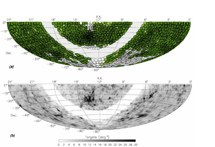
In total, there are 1564 fields and 174 442 galaxies in the 6dFGS, yielding a mean source density of 112 galaxies per field. With an instrument field size of 25.5  deg² and 10.2 sources  deg^-2, the field tiling has effectively had to cover the southern sky twice over. Figure 1 shows the survey coverage to date from the 1 390 fields contributing to the LFs herein. Although substantial areas at mid- and equatorial declinations have been covered, some areas await a second pass, and as a result, redshift completeness will ultimately be higher. Coverage around the Pole is still largely incomplete, but will be addressed during the closing stages of the survey.

Targets for the 6dFGS were selected from the 2MASS Extended Source Catalog (2MASS XSC; Jarrett et al., 2000) for southern declinations $\delta<0^{\circ}$ and at galactic latitudes $|\,b\,|>10^{\circ}$ for $JHK$ and $|\,b\,|>20^{\circ}$ for $b_{\rm\scriptscriptstyle J}r_{\rm\scriptscriptstyle F}$. Table 1 summarises the selection criteria, sample sizes and sky coverage. The motivations for the sample selection criteria are outlined in Jones et al. (2004).

Total magnitudes are the preferred way of quantifying galaxy flux because the related observable (total luminosity) is more physically meaningful than isophotal or aperture magnitudes that depend on selection criteria or distance. At the time the target lists were prepared, however, the total $K$ magnitudes ($K_{\rm tot}$) from the 2MASS XSC were not sufficiently reliable at the lowest galactic latitudes in the survey due to insufficient depth and spatial resolution. The isophotal 2MASS $K$ magnitudes ($K_{\rm iso}$) were more robust, however, and so formed the basis for a derived $K_{\rm tot}$ that we used for target selection in $K$:

$$K_{\rm tot}=K_{\rm iso}-1.5\exp{[1.25(\overline{\mu_{K20}}-20)]}.$$ (1)

Here, $\overline{\mu_{K20}}$ is the mean surface brightness within the $\mu_{K}=20$ elliptical isophote. The scatter in $(\mbox{$K_{\rm iso}$}\ -\mbox{$K_{\rm tot}$})$ is typically no more than 0.1 to 0.2 magnitudes over the range of surface-brightnesses encountered (Fig. 1 of Jones et al., 2004).

This correction was eventually superseded by the revised total $K$ magnitudes from 2MASS XSC which became available after 6dFGS observations had commenced. These show less scatter than the $K_{\rm tot}$ values used for the 6dFGS sample selection (T. Jarrett, priv. comm.) and are a superior measure of total flux.

Both the old and new magnitudes contribute to the 6dFGS luminosity functions in different ways. The original $K_{\rm tot}$ magnitudes are preserved for selection purposes and were used for deriving the selection function and completeness corrections (Sect. 2.3). However, the superior $K$ magnitudes are used to compute galaxy luminosities after all selection cuts and completeness corrections have been made.

The first studies to use 2MASS photometry for LF work were divided over the use of isophotal (Kochanek et al., 2001) or total magnitudes (, Cole et al.2001). While Kochanek et al. claimed their $(\mbox{$K_{\rm iso}$}-\mbox{$K_{\rm tot}$})$ correction was only 0.20 mag, Andreon (2002) argued that it is closer to 0.3 mag. Claims that differences between the optical SDSS and 2MASS NIR luminosity densities were due to a 2MASS bias against low surface brightness systems (Wright, 2001) were largely countered when the SDSS optical luminosities were re-computed to include galaxy evolution (Blanton et al., 2003), although a small offset remains.

(Cole et al.2001) have undertaken a comparison of their adopted 2MASS Kron and extrapolated magnitudes with the deeper infrared photometry of Loveday (2000). They found scatter of around $\sigma\approx 0.13$–0.14 magnitudes in both samples, although found that this reduced to $\sigma\approx 0.1$ if $K$ Kron magnitudes were derived from higher quality $J$ data and $(J-K)$ colours. Likewise, Bell et al. (2003) find a scatter if $\sim 0.2$ mag in comparisons of 2MASS Kron magnitudes with those of Loveday (2000). Since these studies, the 2MASS photometry has been revised. With the current total magnitudes, we find $\langle\mbox{$K_{\rm iso}$}-\mbox{$K_{\rm tot}$}\rangle=0.08$ for $\mbox{$K_{\rm iso}$}\lesssim 10$, rising to $\langle\mbox{$K_{\rm iso}$}-\mbox{$K_{\rm tot}$}\rangle=0.12$. At $\mbox{$K_{\rm iso}$}\gtrsim 11$, the corrections can be as large as 0.5 mag, reflecting the lower surface brightness late-type galaxies that populate this regime. Eke et al. (2005) find that the improved 2MASS total magnitudes match the Loveday data with a scatter of 0.125 mag.

The original $b_{\rm\scriptscriptstyle J}r_{\rm\scriptscriptstyle F}$ samples for 6dFGS were selected from the SuperCOSMOS catalogue in 2001. This photometry suffered from scatter in the field-to-field zeropoints of a few tenths of a magnitude. After the all-sky digital photometry of 2MASS subsequently became available, the original $b_{\rm\scriptscriptstyle J}$, $r_{\rm\scriptscriptstyle F}$ (and $i_{\rm N}$) SuperCOSMOS magnitudes were re-calibrated in 2003 to a common zeropoint by J. Peacock, N. Hambly and M. Read, for the benefit of the 2dF Galaxy Redshift Survey. Individual field zeropoints were characterised by the mean $(\mbox{$b_{\rm\scriptscriptstyle J}$}\ -J)$ colour. The revised SuperCOSMOS magnitudes show a significant improvement in the photometric calibration, with zeropoint scatter of 0.04 mag rms in each band (Cole et al., 2005). Cross et al. (2004) find a scatter of $\sigma=0.1$ mag in a comparison of the revised SuperCOSMOS magnitudes with the CCD photometry of the Millennium Galaxy Catalogue and Sloan Early and First Data Releases (Stoughton et al., 2002; , Abazajian et al.2003).

As with the revised $K$ photometry, the original $b_{\rm\scriptscriptstyle J}r_{\rm\scriptscriptstyle F}$ magnitudes were retained for selection and completeness calculations while the re-calibrated ones were used for luminosities. This is similar to the approach used by the 2dFGRS when re-calibrated $b_{\rm\scriptscriptstyle J}$ photometry became available mid-way through that survey (Norberg et al., 2002; Cole et al., 2005). However, in that case, the new and old magnitudes were related by a simple transformation which imparted no additional scatter. In the case of 6dFGS, the relationship between the old and new magnitudes is not as straightforward. However, the scatter that results is small and inconsequential, largely because the dataset itself remains the same.

Table 1: 6dFGS target samples

Sample Selection	Full Sample			This Paper
	Total	Additional	Area	Number	Effective Area
	Number	to $K$ sample	(deg2)	Used	(deg2)
2MASS $K<12.75$	113 988	–	17 045	60 689	9 075
2MASS $H<13.00$	90 407	3 282	17 045	53 142	10 019
2MASS $J<13.75$	93 925	2 008	17 045	55 236	10 024
SuperCOSMOS $\mbox{$r_{\rm\scriptscriptstyle F}$}<15.60$	66 904	9 199	13 572	37 156	7 537
SuperCOSMOS $\mbox{$b_{\rm\scriptscriptstyle J}$}<16.75$	64 138	9 749	13 572	37 128	7 857

2.2 Surface Brightness Issues

One common misgiving surrounding apparent magnitude limited surveys is the extent to which they bias the LF against low surface brightness systems (Disney, 1976; Impey & Bothun, 1997; Sprayberry et al., 1997; Dalcanton, 1998). Analyses utilising bivariate brightness distributions find $\lesssim 1$ mag arcsec^-2 change in the peak surface brightness for the $b_{\rm\scriptscriptstyle J}$-selected 2dF Galaxy Redshift Survey across observed luminosities (Cross et al., 2001; Driver, 2004), while Cross & Driver (2002) claim that the faint-end slope is robust to surface brightness effects.

In the case of the 2MASS XSC, (Cole et al.2001) have modelled the selection characteristics following the methods of Cross et al. (2001) and Phillipps, Davies & Disney (1990), and find no selection bias against low surface brightness galaxies by 2MASS. Specifically, they demonstrate that their galaxies lie well within the theoretical maximum volumes corresponding to their apparent magnitude and surface brightness limits ($\mbox{$J$}=14.45$ and 20.5 mag arcsec^-2 respectively). The claims by Bell et al. (2003) that surface brightness selection impacts the $K$-band LF are based on brighter surface brightness limits ($\mu_{K}=17$ to 20) than the $\mu_{K}=20$ limit of the 6dFGS.

Taken together, these results imply that at the magnitudes used by the 6dFGS, 2MASS is virtually unaffected by bias against low surface brightness galaxies . The 6dFGS magnitude limits are $\sim 1.5$ mag brighter than the incompleteness regime for the 2MASS XSC, ensuring an effective compromise between sensitivity and robust selection for the redshift survey sample.

2.3 Selection Function

The probability of obtaining a redshift for a galaxy is expected to depend on its apparent magnitude $K$: the fainter it is, the less the chance that its redshift will be secured. However, in a survey such as 6dFGS, the basic observable units are not the galaxies, but the fields to which they belong. Therefore, the probability that a galaxy redshift will be obtained depends not only on its apparent magnitude, but also on the overall redshift success rate of its field.

The survey selection function gives the survey redshift completeness as function of both magnitude and sky position. In short, it is obtained by taking each 6dFGS field and fitting a functional form to the decline in completeness with magnitude (Colless et al., 2001; Norberg et al., 2002). This form is then normalised to reproduce the overall redshift completeness at that point in the sky.

Figure 2: Generalised field completeness and its dependence on apparent magnitude (solid points with error bars) for fields in the ranges ($a$) $0.9<R_{f}\leq 1.0$, (set $F=1$), ($b$) $0.8<R_{f}\leq 0.9$, ($F=2$), ($c$) $0.7<R_{f}\leq 0.8$, ($F=3$), and ($d$) $0.6<R_{f}\leq 0.7$, ($F=4$). The magnitude bin widths (dotted histogram) and individual fit components (dashed curves) are also shown.

Before we can compute the survey selection function we must first determine the general form for completeness as a function of magnitude for each band $KHJr_{\rm\scriptscriptstyle F}b_{\rm\scriptscriptstyle J}$, modulo field completeness. Figure 2 shows how this varies if we divide galaxies into one of four groups:

1. galaxies from high quality fields with completeness in the range $0.9<R_{f}\leq 1.0$ (denoted set $F=1$);

2. galaxies from lower quality fields with $0.8<R_{f}\leq 0.9$ ($F=2$);

3. galaxies from mediocre fields with $0.7<R_{f}\leq 0.8$ ($F=3$);

4. galaxies from poor fields with $0.6<R_{f}\leq 0.7$ ($F=4$).

The completeness, $R(f)$, of field $f$ was determined as

$$R(f) = \frac{N_{z}(f)}{N_{p}(f)}$$ (2)

$$= \frac{N_{{\rm lit}}(f)+N_{{\rm 6dF}}(f)}{N_{{\rm lit}}(f)+N_{{\rm 6dF}}(f)+N_{\rm f}(f)+N_{\rm r}(f)}.$$

Here, $N_{z}(f)$ is the number of extragalactic redshifts obtained in the field, $f$, and $N_{p}(f)$ is the number of confirmed-extragalactic and yet-to-be-observed sources from the parent catalogue. $N_{\rm f}(f)$ and $N_{\rm r}(f)$ are the number of redshift failures and sources remaining to be observed, respectively. $N_{{\rm lit}}(f)$ and $N_{{\rm 6dF}}(f)$ count the literature and 6dF-measured redshifts within each field boundary, respectively. Around one-eighth of our redshifts come from the literature, mainly Huchra’s ZCAT Catalog (Huchra et al., 1992) or the 2dFGRS (Colless et al., 2001) in the ratio $4:1$ respectively. While observing for 2dFGRS is complete, ZCAT continues to be supplemented by the Two Micron All-Sky Redshift Survey (2MRS; Huchra et al., 2006), which to date has obtained around 20 k redshifts to $\mbox{$K$}=11.25$ across the full sky. Sources for which spectra were obtained, and which were found to be stars, planetary nebulae, Hii regions, or other Galactic objects, were excluded.

At $\mbox{$b_{\rm\scriptscriptstyle J}$}\lesssim 16.0$ ($\mbox{$K$}\lesssim 12$), ZCAT redshifts represent more than one-third of the sample. As a consequence, completeness below the 2MRS limit is comparatively high while the 6dFGS continues to fill out completeness at fainter magnitudes ($\mbox{$K$}\gtrsim 11.25$). This dual redshift contribution is evident in our measurements of completeness as a function of magnitude, which exhibit a bump in the declining portion of the curve (Fig. 2).

The generalised completeness curves were fit by a double-exponential,

$$C_{F}(m) = \beta_{F}\,{\rm max}[0,1-\exp{(m-\mu_{F})}]$$ (3)

$$+(1-\beta_{F})\,{\rm max}[0,1-\exp{(m-\xi_{F}})].$$

The motivation for this model was the single exponential form adopted by 2dFGRS (Colless et al., 2001), modified to a double-exponential to fit the shoulder. Table 2 lists the fit parameters $\beta_{F}$, $\mu_{F}$ and $\xi_{F}$ according to passband and field group ($F=1,2,3$ or 4). The shoulder occurs at $\xi_{F}$ values typically 0.5 to 0.75 mag brighter than the survey limits. In the near-infrared bands, the initial decline in completeness is steeper than Eqn. (3) can match. We experimented with fitting a single exponential model and in Sect. 4.1 we demonstrate that the luminosity functions are unaffected by deviations of this size from the fit. Individual uncertainties in Fig. 2 were computed as follows. Given that completeness is the ratio of $N_{z}$ successful redshifts to $N$ sources measured, then the uncertainty in completeness per bin is

$$\Delta C=\frac{\sqrt{N(N_{z}+2)(N-N_{z}+1)}}{N(N+3)}.$$ (4)

Table 2: Magnitude-dependent completeness parameters Parameters describing the best analytic fit to the magnitude-dependent completeness in Eqn. (3).

Field Completeness	Field	$\beta_{F}$	$\mu_{F}$	$\xi_{F}$
	Set $F$		(mags)	(mags)
$K$-band:
$0.9<R_{f}\leq 1.0$	1	0.80	14.84	12.03
$0.8<R_{f}\leq 0.9$	2	0.74	14.72	11.96
$0.7<R_{f}\leq 0.8$	3	0.71	14.90	12.03
$0.6<R_{f}\leq 0.7$	4	0.70	15.02	12.20
$H$-band:
$0.9<R_{f}\leq 1.0$	1	0.85	14.66	12.27
$0.8<R_{f}\leq 0.9$	2	0.79	14.60	12.20
$0.7<R_{f}\leq 0.8$	3	0.70	15.12	12.39
$0.6<R_{f}\leq 0.7$	4	0.87	14.24	12.37
$J$-band:
$0.9<R_{f}\leq 1.0$	1	0.83	15.56	12.99
$0.8<R_{f}\leq 0.9$	2	0.78	15.32	12.97
$0.7<R_{f}\leq 0.8$	3	0.79	15.14	13.11
$0.6<R_{f}\leq 0.7$	4	0.84	15.20	12.87
$r_{\rm\scriptscriptstyle F}$-band:
$0.9<R_{f}\leq 1.0$	1	0.92	16.96	15.04
$0.8<R_{f}\leq 0.9$	2	0.86	16.96	14.92
$0.7<R_{f}\leq 0.8$	3	0.83	17.25	15.16
$0.6<R_{f}\leq 0.7$	4	0.71	20.00	14.92
$b_{\rm\scriptscriptstyle J}$-band:
$0.9<R_{f}\leq 1.0$	1	0.87	18.29	16.10
$0.8<R_{f}\leq 0.9$	2	0.81	18.47	16.22
$0.7<R_{f}\leq 0.8$	3	0.78	18.54	16.22
$0.6<R_{f}\leq 0.7$	4	0.70	21.29	16.40

With the form of the magnitude-dependent completeness known, we are in a position to determine total completeness, $T_{F}(\mn@boldsymbol{\theta},m)$, as a function of both sky position $\mn@boldsymbol{\theta}$ and magnitude $m$. We assume it is separable function with the general form

$$T_{F}(\mn@boldsymbol{\theta},m)=S(\mn@boldsymbol{\theta})\cdot C_{F}(m),$$ (5)

for all galaxies in a given field group $F$. $S(\mn@boldsymbol{\theta})$ is a constant scaling the completeness of the individual field to that of the total completeness in the same part of sky,

$$S(\mn@boldsymbol{\theta})=R(\mn@boldsymbol{\theta})\cdot\frac{\int_{m_{\rm bright}}^{m_{{\rm faint}}}\overline{N(m)}\,\,dm}{\int_{m_{\rm bright}}^{m_{{\rm faint}}}C_{F}(m)\cdot\overline{N(m)}\,\,dm}.$$ (6)

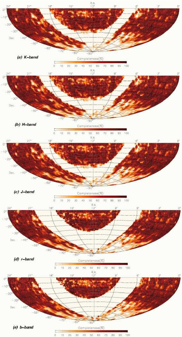
Actual sky completeness, $R(\mn@boldsymbol{\theta})$, is the ratio of extragalactic redshifts ($cz\geq 750\mbox{\,km\,s${}^{-1}$}$) at sky position $\mn@boldsymbol{\theta}$, to the number of confirmed or potentially extragalactic sources at the same position. It is measured in exactly the same manner as field completeness $R(f)$, except on a uniform $1.5^{\circ}$ grid of circular regions of diameter $2^{\circ}$. This geometry was unrelated to the placement of actual 6dFGS fields or the way in which they overlapped. Figure 3 shows the redshift completeness of the all $KHJr_{\rm\scriptscriptstyle F}b_{\rm\scriptscriptstyle J}$ samples. Typically there is little variation between bands.

Figure 3: Actual survey completeness on the sky, $R(\mn@boldsymbol{\theta})$, for each of the $KHJr_{\rm\scriptscriptstyle F}b_{\rm\scriptscriptstyle J}$ samples used in this paper.

$\overline{N(m)}$ is the mean number of galaxies per magnitude per field area, which we derive in Section 3.1. The magnitude limits of the survey are given by $m_{{\rm bright}}$ and $m_{{\rm faint}}$.

In the case of the $1/V_{\rm max}$ luminosity estimator (Schmidt, 1968), the inverse of the total completeness, $(T_{F}(\mn@boldsymbol{\theta}_{i},m_{i}))^{-1}$, is used to weight the inverse maximum accessible volume of each galaxy $i$. For the STY Sandage, Tammann & Yahil (1979) and SWML (Efstathiou, Ellis & Peterson, 1988) estimators, $T_{F}(\mn@boldsymbol{\theta},m)$ is re-expressed in terms of absolute magnitude $M$ for each galaxy using

$$M=m-5\log[d_{L}(z_{i})]-25-k(z_{i}).$$ (7)

Here, $d_{L}(z_{i})$ is the luminosity distance in Mpc, $k(z_{i})$ is the $k$-correction and $z_{i}$ the redshift of the $i$th galaxy. Equation (7) is written in a form that ignores the evolutionary corrections that become significant at higher redshift. $T_{F}(\mn@boldsymbol{\theta},M)$ then weights the number density for all $M$.

3 Luminosity Function Preliminaries

3.1 Number Counts and Normalisation

Large scale structure plays an important role in defining the overall normalisation of any LF, and is a crucial factor in determining the optimal depth and sky coverage of the survey. Arguably it is the single biggest contributor to discrepancies between recent LFs and related quantities (see e.g. , Cole et al.2001; Norberg et al., 2002; Bell et al., 2003; Driver, 2004; Driver et al., 2005). While recent luminosity function determinations have been able to exploit surveys of unprecedented depth and coverage, cosmic structure is always an issue for the faintest galaxies of any survey. estimate that cosmic variance could introduce systematic errors as large as 15 percent in number counts from their sample combining 2MASS NIR photometry with 2dFGRS redshifts. Bell et al. (2003) has found the SDSS Early Data Release to be 8 percent overdense with respect to the 2MASS extended source counts over the whole sky, and the 2dFGRS to be slightly under-dense.

To date, the 6dFGS has covered about a quarter of the sky, or $\sim 2$ to 3 sr depending on passband. Compared to recent near-infrared ($K$-band) samples, the 6dFGS currently covers about $\sim 15$ to 20 times the area of (Cole et al.2001) and Bell et al. (2003) and around 30 percent more that of Kochanek et al. (2001). In terms of sample size, the 6dFGS is $\sim 10$—15 times larger than Kochanek et al. (2001) and Bell et al. (2003) and a factor of 4 greater than (Cole et al.2001). At optical magnitudes, current 6dFGS sky coverage quadruples that used for the 2dFGRS Norberg et al. (2002) and SDSS Blanton et al. (2003) luminosity functions, although sample size is roughly half. When complete, the sky coverage of 6dFGS will be almost double its present extent.

Figure 4: Differential number counts for the $KHJr_{\rm\scriptscriptstyle F}b_{\rm\scriptscriptstyle J}$ samples of the 6dFGS. The Euclidean slope of 0.6 has been subtracted for emphasis. Magnitudes have been corrected for Galactic extinction and are expressed as an offset from each survey limit (indicated). The solid lines show the straight lines of best fit given in Table 3. Poisson errors are shown.

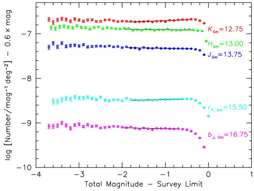
Figure 4 shows the differential number counts for 6dFGS sources after correction for Galactic extinction (Sect. 3.4). The roll-over near the survey limit is the result of the extinction corrections blurring the sharp survey cut-offs imposed on the original uncorrected magnitudes. Unlike imaging number count surveys, we have been able to use our redshift information to remove stellar contamination from the counts. The counts were averaged over the effective area of the 6dFGS, obtained by scaling the eventual survey area by the fraction of targets in hand. Table 3 gives our linear least-squares fit parameters $a,b$ for the form

$$N(m)=10^{am+b}$$ (8)

where $m$ is magnitude and $N(m)$ is the differential surface density (  mag^-1 deg^-2). The counts are flat in all bands with the exception of $K$, (and to a lesser extent, $r_{\rm\scriptscriptstyle F}$). This rise has also been seen in the 2MASS number counts published previously (e.g. , Cole et al.2001; Jarrett, 2004), and was initially thought to be due to the well-known upwards bias of number count data in regimes of declining signal-to-noise (Murdoch, Crawford & Jauncey, 1973). We tested this by generating artificial random samples with the same size, flux and error distribution of the real $K$-band sample. This Monte-Carlo approach revealed that even uncertainties as large as $\mbox{$\Delta K$}\sim 0.2$ were unable to raise a nominal Euclidean 0.6 slope by more than 1 percent. Typical 2MASS flux errors are closer to $\mbox{$\Delta K$}\sim 0.1$ at $\mbox{$K$}=12.5$. It is possible that the rise in $K$ reflects the fact that the fainter bins are capturing more of the intrinsically lower surface brightness late-type galaxies, although no such rise is seen in the higher signal-to-noise $H$ or $J$ counts.

Our source density of 3.2 galaxies  mag^-1 deg^-2 at $\mbox{$K$}=12.5$ is comparable to the 3  mag^-1 deg^-2 found by Bell et al. (2003) and (Cole et al.2001) for the 2MASS XSC in Kron magnitudes. These are typically 0.1 to 0.2 mag brighter than the original total magnitudes of 2MASS (, Cole et al.2001), although it should be noted that the total magnitudes we now use for 6dFGS are the recently revised ones (Jarrett, priv. comm.). The 6dFGS number counts are identical to 2MASS number counts at $\mbox{$K_{\rm iso}$}=12.2$ (Jarrett, 2004), allowing for the fact that 2MASS isophotal magnitudes are typically 0.1 to 0.2 mags fainter than total magnitudes. Like Bell et al., we find that the Sloan Early Data Release counts are somewhat higher than average (3.5  mag^-1 deg^-2; Bell et al., 2003), the likely result of an overdensity in its comparatively smaller survey region (370 deg²). In the optical, the 6dFGS $b_{\rm\scriptscriptstyle J}$-band counts of 2.9  mag^-1 deg^-2 ($\mbox{$b_{\rm\scriptscriptstyle J}$}=16.0$) are closer to the 2dFGRS counts in the SDSS–2dFGRS overlap region (2.9  mag^-1 deg^-2; Norberg et al., 2002), although the NGP and SGP 2dFGRS regions (3.3  mag^-1 deg^-2) remain within the errors. Ultimately, such comparisons are limited by the systematics of different galaxy photometry techniques and magnitude definitions.

Table 3: Best fit parameters to extinction-corrected 6dFGS number count data.

Band	Fit range		Number of	Fit Parameters
	(mag)	(mag)	sources	$a$	$b$
$K$	10.75	12.35	113988	0.636	-7.132
$H$	10.95	12.65	90317	0.588	-6.769
$J$	11.75	13.40	93831	0.583	-7.114
$r_{\rm\scriptscriptstyle F}$	13.60	14.90	64043	0.621	-8.782
$b_{\rm\scriptscriptstyle J}$	14.70	16.10	66833	0.577	-8.769

3.2 Disentangling Hubble and Peculiar Motions

The line-of-sight velocity measured for a galaxy has two components: the Hubble flow due to the expansion of the universe, and the peculiar velocity due to the combined gravitational attraction of all large-scale structures. To infer true luminosity distances from the Hubble flow velocity, (assuming $z\ll 1$; Hubble, 1934), we must first remove the peculiar motion component, especially given the low redshifts for much of our sample.

We have adopted field flow corrections from software written by J. P. Huchra for the HST Key Project to measure $H_{0}$ (Appendix A of Mould et al., 2000). This uses a simple linear flow field with three spherical mass concentrations representing Virgo ($cz=1\,035\mbox{\,km\,s${}^{-1}$}$), the Great Attractor (GA; $4\,600\mbox{\,km\,s${}^{-1}$}$) and the Shapley Supercluster (SSC; $13\,800\mbox{\,km\,s${}^{-1}$}$). We also examined the flow models of Tonry et al. (2000) and Burstein et al. (1989), but did not use them since they neglect the SSC, which is a significant influence on much of the 6dFGS volume.

Figure 5: Change in magnitude resulting from peculiar velocity corrections in two key sky directions (the Great Attractor and Shapley Supercluster, $a$ and $b$), and for the entire 6dFGS sample ($c$). These show the difference between absolute magnitudes derived from the flow-model-corrected $cz$ values and uncorrected $cz$ values. The diagonal bands are galaxies that the model has identified with the Great Attractor ($4\,600$ km s^-1) or Shapley Supercluster ($\sim 13\,800$ km s^-1) mass concentrations, and ascribed the corresponding systemic velocity.

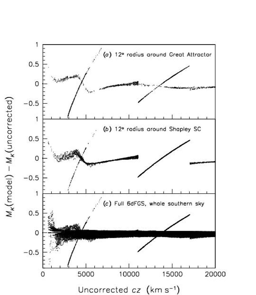
Peculiar velocity corrections are most significant for $cz\lesssim 10\,000$ km s^-1. Figure 5 shows how removal of the peculiar motion alters the absolute magnitudes for galaxies in the direction of the GA and SSC. The Virgo cluster direction is not shown, as it lies beyond the northern limits of the 6dFGS. In the vicinity of the GA, galaxy luminosities are affected by as much as $\pm 0.2$ mags while for the SSC the effect is clearly less ($\lesssim 0.1$ mag). For galaxies within either mass concentration, the correction can be almost a magnitude. This is because the flow model sets the galaxy velocity to that of the mass concentration if the galaxy lies within its sphere of influence.

With median redshifts in excess of 20 000 km s^-1, most recent surveys do not include corrections for peculiar velocities. An exception is Kochanek et al. (2001), who employed the local flow model of Tonry et al. (2000). Kochanek et al. also employ a low-$cz$ cut-off of 2000 km s^-1, so as to exclude those local galaxies with a significant dependence on flow corrections, at the expense of 5 percent of their sample and $\sim 1.5$ mags at their faint-end limit.

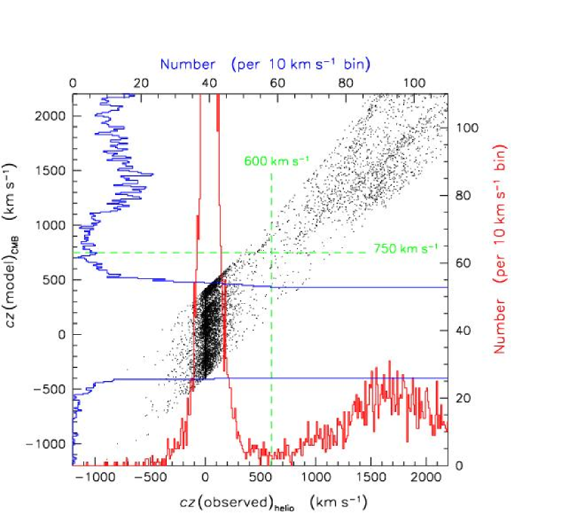
The nominal 6dFGS low-$cz$ cut-off is 600 km s^-1, set so as to separate the obvious peak in Galactic sources at $cz\approx 0$ km s^-1 from the rising redshift distribution of true extragalactic objects (Fig. 6). However, applying the flow model corrections broadens the distribution of all velocities, including those sources that are quite clearly Galactic. Therefore, we adjust the low-$cz$ limit to 750 km s^-1 and use this throughout as our minimum acceptable redshift cut-off. Galaxies above the cut-off are used with their flow-corrected velocities from the model.

Figure 6: Effect of flow model on low $cz$ values in relation to the low-$cz$ cut-off. The points show observed and model velocities relative to the lower and left-hand axes. The histograms show how the distribution projects along the same directions relative to the vertical scales shown on the right and above. The dashed lines indicate our low-$cz$ cut-off for both observed (600 km s^-1) and model-corrected $cz$ values (750 km s^-1).

3.3 Effect of Magnitude Errors

The 6dFGS has been able to take advantage of the emerging availability of quality photometry over large areas of the sky. This is particularly the case for the NIR, where the digital 2MASS photometry of the whole sky permits a uniformity and precision unprecedented in wide area redshift surveys. With this kind of precision, we are motivated to examine whether photometric errors modify the shape of the luminosity distribution, and if so, by how much. For example, a non-gaussian tail in the error distribution can influence the bright end of the LF due to its rapid decline in this region.

Figure 7: Distribution of $JHK$ photometry uncertainties for the revised 2MASS total magnitudes (points). The large solid blue points and long-dashed blue line both trace the $1\sigma$ deviation of the uncertainties when grouped into 0.5-mag bins. The vertical solid red curves are half-gaussian representations of the same $1\sigma$ deviation. The vertical short-dashed lines indicate the nominal 6dFGS magnitude limits in each band. There are a small number of galaxies fainter than this limit due to the improvements to photometry after target selection.

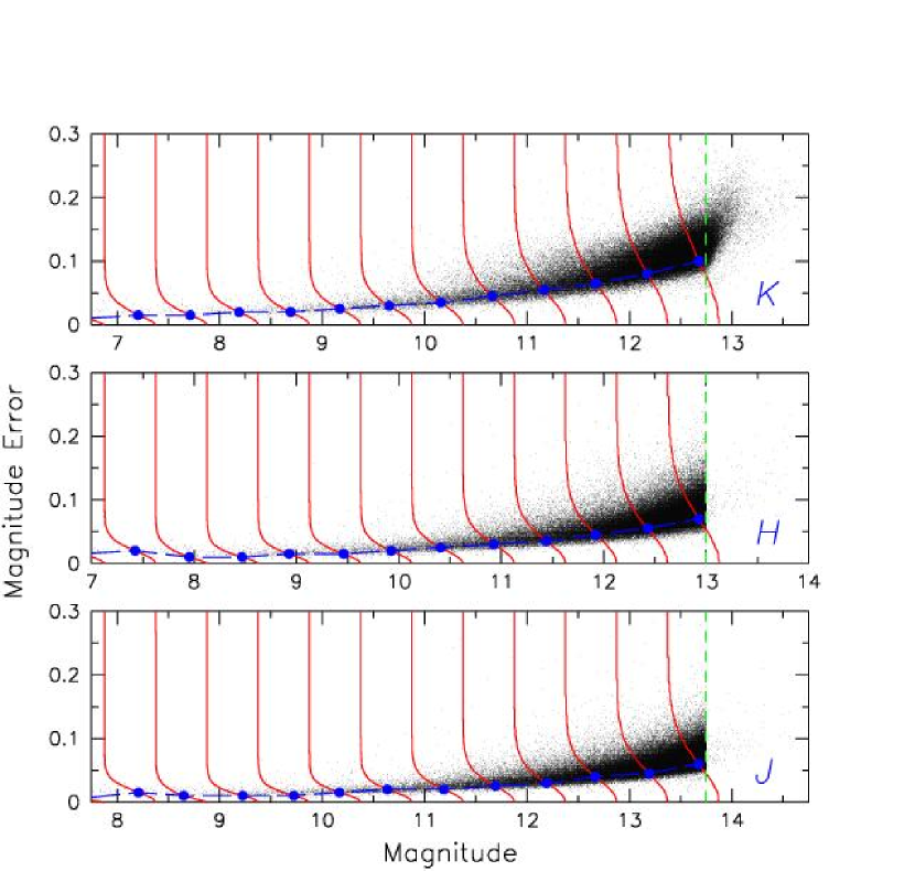
Figure 7 shows 2MASS photometric errors for $JHK$ for 6dFGS targets. Typical errors are $\sim 0.1$ mag in $K$ and $\sim 0.06$ to 0.08 mag in $J$ and $H$. In terms of absolute magnitude, these translate fairly uniformly across the range of observed luminosities (Fig. 8). Because of this, we apply the mean photometric error ($\sigma=0.108,0.083$ and 0.065 for $KHJ$ respectively) to all luminosities equally when computing its effect on the LF. Uncertainties in $b_{\rm\scriptscriptstyle J}$ and $r_{\rm\scriptscriptstyle F}$ are typically $\sim 0.1$, comparable with $K$.

The functional form most commonly used to match the galaxy luminosity distribution is that proposed by Schechter (1976), which gives the space density of galaxies per unit absolute magnitude, $\phi(M)$, as

$$\phi(M)\,dM=0.4\ln 10\,\mbox{$\phi_{*}$}\,\frac{(10^{0.4(M_{*}-M)})^{\alpha+1}}{\exp[10^{0.4(M_{*}-M)}]}\,dM.$$ (9)

The parameter $\phi_{*}$ is a normalisation constant, while $\alpha$ is the slope for faint galaxies and $M_{*}$ is a characteristic magnitude at the transition from the exponential to power law dependence. While both the Schechter Function and Press-Schechter Mass Function (Press & Schechter, 1974) are superficially similar, they are not related in any simple physical way. The exponential cutoff at the bright end of the Schechter Function is due to cooling (e.g. Rees & Ostriker, 1977) and perhaps feedback by AGN. If it were caused only by the high mass cutoff of the Press-Schechter Function then $M_{*}$ would be $\sim 4$ magnitudes brighter.

Figure 8: Distribution of $JHK$ photometric errors as a function of absolute total magnitude. The vertical lines are the result of dividing galaxies into 0.22-mag bins and co-adding gaussians equal to the $1\sigma$ magnitude errors of the relevant galaxies. The short dashed lines indicate the $\pm 1\sigma$ deviation and the long dashed histogram shows the distribution of 6dFGS sources on the same scale of absolute magnitude. The right-hand panels show the superposition of magnitude distributions for each bin (dotted lines) with the average for all shown by the solid line. The $\sigma$ for this distribution is indicated uppermost in each panel.

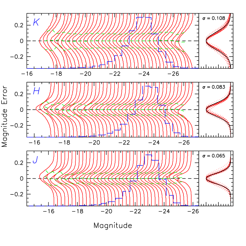
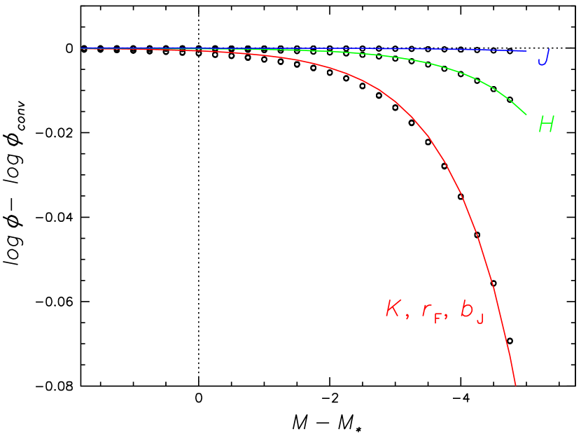
In order to explore the effect of magnitude errors on this analytic fit, we convolved Schechter functions across a range of $\alpha$ values with the gaussian error kernels discussed above. Figure 9 shows how a generic Schechter function changes in $\log\phi$-space when convolved with gaussian magnitude distributions of $\sigma=0.07$ to 0.1. As expected, only the brightest luminosities in the region $M<\mbox{$M_{*}$}$ are affected. Perhaps more surprising is that the amount of change is highly insensitive to the faint-end slope $\alpha$ for typical values. In the case of $J$, the magnitude errors are too small to have any appreciable effect on the Schechter fit. In the interests of computational efficiency we have used the empirical relationship

$$\log\mbox{$\phi_{\rm conv}$}=\log\phi+e^{M_{*}-M-\upsilon}$$ (10)

with values of $\upsilon=7.37$ to match the convolution offsets in $K$$r_{\rm\scriptscriptstyle F}$$b_{\rm\scriptscriptstyle J}$, 9.15 for $H$, and 12.25 for $J$. Figure 9 shows each of these curves. These offsets were then applied when finding optimal Schechter function fits in all bands (Section 4).

3.4 Extinction and Cosmological Corrections

One of the primary science drivers for the NIR selection of the main 6dFGS samples was the low impact of Galactic extinction over much of the sky. We use the maps of Schlegel, Finkbeiner & Davis (1998) to correct our total magnitudes using the relative extinction values of $A/A_{V}=0.112,0.176,0.276,0.810,1.236$ for $KHJr_{\rm\scriptscriptstyle F}b_{\rm\scriptscriptstyle J}$ respectively. Typically this furnishes extinction corrections of up to $\sim 0.04$ mag in $K$, $\sim 0.1$ mag in $J$, and $\sim 0.3$ in $b_{\rm\scriptscriptstyle J}$ (recall that the respective Galactic latitude limits are $|\,b\,|>10^{\circ}$ for $JHK$ and $|\,b\,|>20^{\circ}$ for $b_{\rm\scriptscriptstyle J}r_{\rm\scriptscriptstyle F}$). Extinction corrections were applied after the initial apparent magnitude selection.

Our cosmological $k$-corrections use the values computed by Poggianti (1997), linearly interpolated with redshift. Given the 6dFGS selection bias towards early-types we adopt her $k$-corrections for an elliptical galaxy with solar metallicity and exponentially decreasing star-formation rate with $e$-folding time of 1 Gyr. These corrections are within 0.1 mag of those used by Kochanek et al. (2001) for their $K$-band sample, and also those of Norberg et al. (2002) for the 2dFGRS $b_{\rm\scriptscriptstyle J}$-band sample.

We do not apply evolutionary $e$-corrections (e.g. Norberg et al., 2002; Blanton et al., 2003), since the bulk of our galaxies are seen at relatively recent cosmic time ($z\lesssim 0.1$).

Figure 9: The open circles show the offset between an ordinary Schechter function ($\log\phi$) and one convolved with the gaussian error kernels for $KHJr_{\rm\scriptscriptstyle F}b_{\rm\scriptscriptstyle J}$ ($\log\mbox{$\phi_{\rm conv}$}$). The result is independent of $\alpha$. The solid lines show the functional form of Eqn. (10) with $\upsilon=7.37$ for $K$$r_{\rm\scriptscriptstyle F}$$b_{\rm\scriptscriptstyle J}$, 9.15 for $H$, and 12.25 for $J$. The vertical dotted line marks the location of $M_{*}$.

4 Luminosity Functions

4.1 6dF Galaxy Survey

Several techniques have been devised over the years for measuring galaxy LFs (see e.g. Willmer, 1997). We have adopted the three most commonly used — $1/V_{\rm max}$, STY and SWML — all of which have merits and shortcomings. The $1/V_{\rm max}$ method (Schmidt, 1968; Felten, 1976) has the advantages of simplicity and no a priori assumption of a functional form for the luminosity distribution. Unlike the others, it also yields a fully normalised solution and is insensitive to magnitude incompleteness. Its main disadvantage is its assumption of a homogeneous, unclustered galaxy distribution. The STY method (Sandage, Tammann & Yahil, 1979) overcomes these difficulties, being a maximum-likelihood estimator with the added advantage that it does not require binning. However, it presupposes some explicit functional model for the luminosity function. The Step-Wise Maximum Likelihood method (SWML; Efstathiou, Ellis & Peterson, 1988) has similar advantages to the STY method, but does not assume an explicit form for the luminosity function. It produces a binned maximum-likelihood estimate of the LF. STY and SWML provide shape information but not the overall normalisation in the manner of $1/V_{\rm max}$. We refer the interested reader to the individual references for detailed methodologies.

Figure 10: Luminosity functions for the 6dF Galaxy Survey, derived from the $1/V_{\rm max}$ (green open circles), SWML (red solid circles) and STY methods (blue dashed curve). The inset shows the 1, 2 and $3\sigma$ confidence contours of the STY fit. The upper panel shows the $1/V_{\rm max}$ and SWML residuals relative to STY (i.e. the deviations from the best-fitting Schechter function).

Table 4: Schechter function parameters for the STY luminosity functions of 6dFGS. The convolution parameter $\upsilon$ used for Eqn. (10) is given for each band.

Sample	Fit Range	$\mbox{$M_{*}$}-5\log h$	$\alpha$	$\log[\mbox{$\phi_{*}$}]$	$\upsilon$
	(mag)	(mag)		($\,h^{3}\,{\rm Mpc}^{-3}$)
$K$	[-15.50,-28.85]	$-23.83\pm 0.03$	$-1.16\pm 0.04$	$-2.126\pm 0.005$	7.37
$H$	[-16.00,-28.50]	$-23.54\pm 0.04$	$-1.11\pm 0.04$	$-2.141\pm 0.005$	9.15
$J$	[-15.00,-27.50]	$-22.85\pm 0.04$	$-1.10\pm 0.04$	$-2.148\pm 0.005$	12.25
$r_{\rm\scriptscriptstyle F}$	[-14.00,-25.00]	$-20.98\pm 0.05$	$-1.21\pm 0.04$	$-2.081\pm 0.006$	7.37
$b_{\rm\scriptscriptstyle J}$	[-12.50,-24.00]	$-19.91\pm 0.05$	$-1.21\pm 0.05$	$-1.983\pm 0.006$	7.37

We have applied the $1/V_{\rm max}$, STY and SWML methods to each of the 6dFGS samples in $KHJr_{\rm\scriptscriptstyle F}b_{\rm\scriptscriptstyle J}$. The STY and SWML LFs were normalised by a $\chi^{2}$ minimisation with respect to the equivalent $1/V_{\rm max}$ distribution.

Sources were excluded if they were outside the redshift range $0.0025<z<0.2$ or had total completeness $T_{F}(\mn@boldsymbol{\theta}_{i},m_{i})<0.6$. Completeness corrections had much less impact on the $1/V_{\rm max}$ results compared to other methods, a point that has been noted by others (e.g. Kaldare, 2001). Those sources with extinction-corrected original magnitudes outside the range $m_{{\rm bright}}$ to $m_{{\rm faint}}$ were also excluded. Here, $m_{{\rm faint}}$ is simply the nominal survey limit $(12.75,13.00,13.75,15.60,16.75)$ corrected for extinction in the direction of the source, while $m_{{\rm bright}}=8.75$, 9.0, 9.75, 13.0, and 14.0 for $KHJr_{\rm\scriptscriptstyle F}b_{\rm\scriptscriptstyle J}$ respectively. Particular care was taken to exclude sources with $\mbox{$r_{\rm\scriptscriptstyle F}$}\lesssim 13$ or $\mbox{$b_{\rm\scriptscriptstyle J}$}\lesssim 14$ because of saturated $r_{\rm\scriptscriptstyle F}$ or $b_{\rm\scriptscriptstyle J}$ photometry in the original Southern Sky Survey plate material. The sizes of the samples actually used in the analysis are given in Table 1.

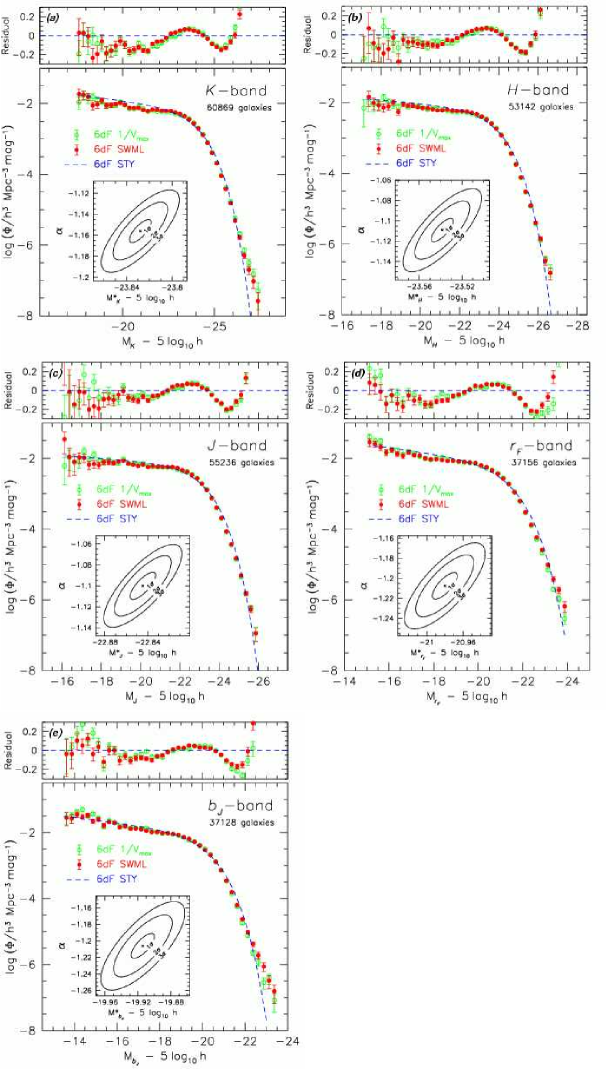
Figure 10 shows the $KHJr_{\rm\scriptscriptstyle F}b_{\rm\scriptscriptstyle J}$ LFs derived for the 6dFGS via these methods. Table 4 summarises the best-fitting error-convolved Schechter functions, while Tables 5 and 6 list the non-parametric $1/V_{\rm max}$ and SWML distributions. All three methods are in excellent agreement, insofar as the Schechter functions represent the data. Moving to bluer passbands we find a slight steepening of the faint-end slope, although not to the extent that has been reported previously for dense environments. This is a consequence of the optical samples harbouring a larger population of late-type galaxies, which are typically of lower luminosity.

The large sample size of the 6dFGS, even at this intermediate stage of the survey, has allowed us to beat down random uncertainties over a considerable range of luminosity. As a consequence, we can clearly see that a Schechter function (Eqn. 9) is only an approximate match to the real galaxy luminosity distribution in all bands (upper panels in Figure 10). Specifically, it is unable to turn over sharply enough around $M_{*}$, and tends to slightly underestimate the true space density of $M_{*}$ galaxies while at the same time slightly overestimating that of $M\sim(\mbox{$M_{*}$}-1.5)$ and $M\gtrsim(\mbox{$M_{*}$}+1.5)$ systems. The differences are typically $\sim 15$ percent around $M_{*}$ and $\sim 30$ to 40 percent beyond. Similar outcomes have been found in the LF fitting of deep SDSS data (Bell et al., 2003; Blanton et al., 2005), prompting these authors to use double Schechter functions, or a hybrid Schechter function plus power law fit.

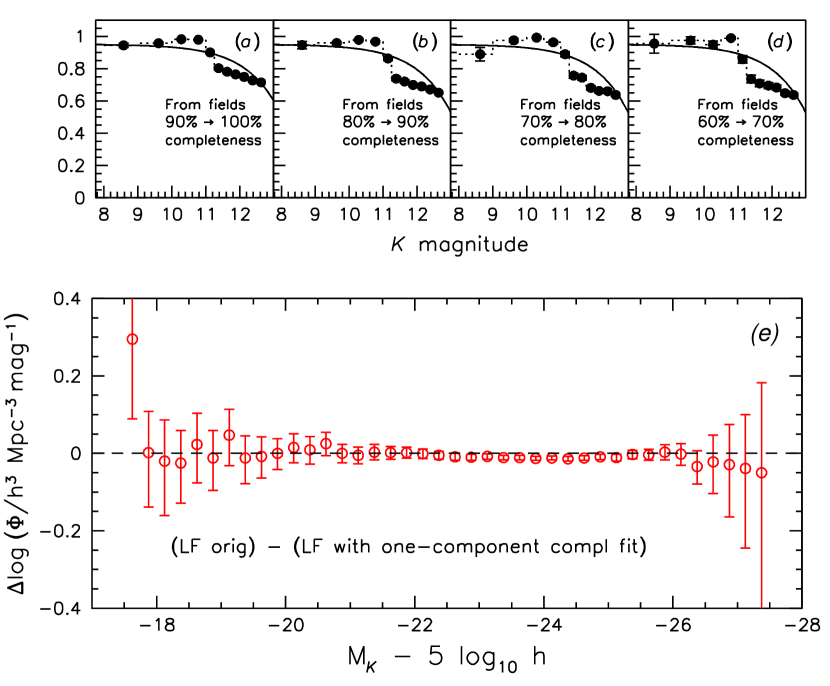
In Sect. 2.3 we claimed that the luminosity function is unaffected by small deviations from the model used to fit the magnitude completeness. Figure 11 shows the result of recomputing the $K$-band luminosity function using a single-component exponential, such as those used by Colless et al. (2001) for 2dFGRS. We find there is negligible change in the luminosity function (Fig. 11$e$), which appears to be fairly insensitive to the exact form used to model magnitude completeness.

Figure 11: Same $K$-band completeness measurements as shown in ($a$) – ($d$) of Fig. 2 (top panel), except fit with a single-component exponential. ($e$) The difference between the luminosity function using these models and that using the double-exponentials of Fig. 2 for $K$. The change is negligible in all bins except the very faintest.

4.2 Luminosity Function Extremities

Figure 12: ($a$) Apparent magnitude-redshift relation for the most luminous members of the $K$-band selected sample ($\mbox{$M_{K}$}<-26.5$). ($b$) Absolute magnitudes in $KHJr_{\rm\scriptscriptstyle F}b_{\rm\scriptscriptstyle J}$ for the same $\mbox{$M_{K}$}<-26.5$ sample. Also shown are the $M_{*}$ values in each band (open circles and dashed line). Cosmological $k$-corrections have been applied.

At faint luminosities $M\gtrsim(\mbox{$M_{*}$}+2)$ we find marginal evidence for an upturn, as has been suggested by a number of authors for clusters (Driver, 2004, and references therein). At the bright end we see a prominent upturn at $M\lesssim(\mbox{$M_{*}$}-2)$, particularly in the $K$ and $b_{\rm\scriptscriptstyle J}$ samples, as has been noted by several authors previously. This excess of luminous objects is presumably due to brightest cluster galaxies, which are produced by the special merger and accretion processes that come into effect in the high density regime at the centre of cluster gravitational potentials. We experimented with fitting this feature using the gaussian LF of Saunders et al. (1990, their Eqn. 6.1), but it only improved the bright-end fit at the expense of poorer fitting elsewhere.

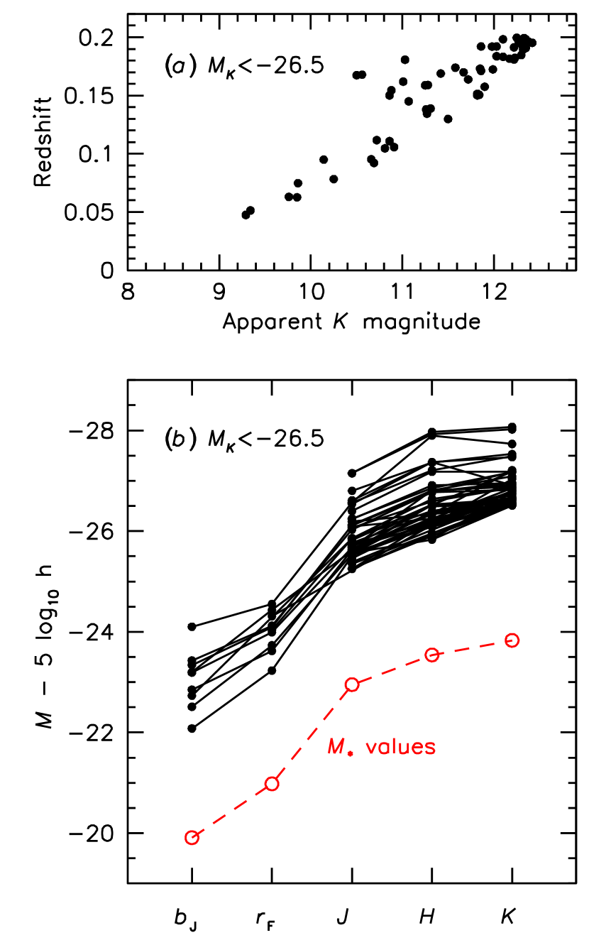
We studied the luminous galaxies responsible for the bright-end upturn in detail. Incorrect redshifts or the presence of a non-gaussian tail on the magnitude error distribution could also cause an upturn if present in our data. Figure 12($a$) shows the magnitude-redshift relation for the most luminous galaxies with $\mbox{$M_{K}$}<-26.5$. It demonstrates that they span a range of of redshift and brightness, as expected for a luminous sample that should be visible over a large survey volume. Figure 12($b$) shows the $k$-corrected absolute magnitudes in $KHJr_{\rm\scriptscriptstyle F}b_{\rm\scriptscriptstyle J}$ for the same sample of galaxies. Some galaxies do not have matching magnitudes in the shorter wavelength bands due to non-selection by the original apparent magnitude cut. Also shown in Fig. 12($b$) is the location of $M_{*}$ in each band. From this we observe that it is the same luminous galaxies that are responsible for the bright-end upturn in all bands. Hence, galaxy membership of the luminous bins is real and not the result of an extended tail in the magnitude error distribution.

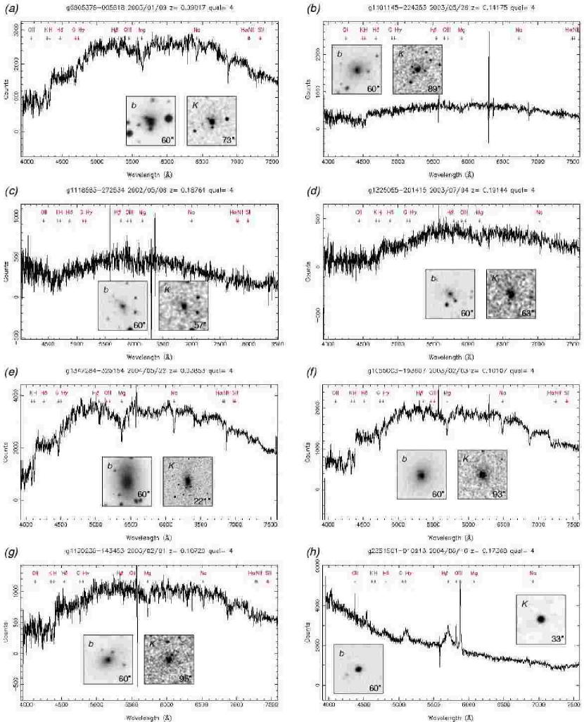
We also paid special attention to the spectra and redshifts of this luminous sample. Figure 13 shows a sub-sample of these with spectra and $b_{\rm\scriptscriptstyle J}$$K$  imaging obtained from the 6dFGS database. Generally, the spectra have signal-to-noise ratios that vary from excellent to poor. This is not surprising given the large range of apparent magnitude seen in Fig. 12($a$). The imaging shows that there are a number of galaxy pairs in this luminous sample. While they are not close enough to have inflated magnitudes due to image mergers — 2MASS can individually identify sources 5 ″ apart — it supports the idea that many of these galaxies inhabit dense environments. In terms of redshift quality, $Q$ (Jones et al., 2004), around half the sample have $Q=4$ indicating that the redshift measurements are secure. Of the remainder, half have $Q=3$ while the other redshifts come from the literature. We can therefore rule out spurious redshifts as a cause of the bright-end upturn.

Figure 13: Spectra of some luminous upturn sources at $\mbox{$M_{K}$}<-26.5$. The labeling of spectral features indicates position only and does not imply detection of the feature. Also shown are postage stamp images in $b_{\rm\scriptscriptstyle J}$ and $K$, taken from SuperCOSMOS and 2MASS respectively. North is up, east is left, and image size is indicated in the lower right-hand corner.

Table 5: Near-infrared $1/V_{\rm max}$ and SWML luminosity functions from the 6dFGS.

$K$-band			$H$-band			$J$-band
$\mbox{$M_{K}$}-5\log h$	$\log[\phi_{\rm vmax}]$	$\log[\phi_{\rm swml}]$	$\mbox{$M_{H}$}-5\log h$	$\log[\phi_{\rm vmax}]$	$\log[\phi_{\rm swml}]$	$\mbox{$M_{J}$}-5\log h$	$\log[\phi_{\rm vmax}]$	$\log[\phi_{\rm swml}]$
(mag)	$(\mbox{$\,h^{3}\,{\rm Mpc}^{-3}$})$	$(\mbox{$\,h^{3}\,{\rm Mpc}^{-3}$})$	(mag)	$(\mbox{$\,h^{3}\,{\rm Mpc}^{-3}$})$	$(\mbox{$\,h^{3}\,{\rm Mpc}^{-3}$})$	(mag)	$(\mbox{$\,h^{3}\,{\rm Mpc}^{-3}$})$	$(\mbox{$\,h^{3}\,{\rm Mpc}^{-3}$})$
$-27.375$	$-7.295\,^{+0.232}_{-0.533}$	$-7.582\,^{+0.233}_{-0.535}$	$-26.625$	$-6.728\,^{+0.131}_{-0.189}$	$-6.818\,^{+0.134}_{-0.194}$	$-25.875$	$-6.932\,^{+0.149}_{-0.228}$	$-6.948\,^{+0.151}_{-0.232}$
$-27.125$	$-6.818\,^{+0.139}_{-0.206}$	$-7.022\,^{+0.140}_{-0.208}$	$-26.375$	$-6.432\,^{+0.090}_{-0.113}$	$-6.474\,^{+0.098}_{-0.127}$	$-25.625$	$-6.233\,^{+0.074}_{-0.089}$	$-6.262\,^{+0.080}_{-0.099}$
$-26.875$	$-6.504\,^{+0.103}_{-0.135}$	$-6.701\,^{+0.104}_{-0.137}$	$-26.125$	$-5.875\,^{+0.052}_{-0.060}$	$-5.845\,^{+0.056}_{-0.064}$	$-25.375$	$-5.823\,^{+0.050}_{-0.057}$	$-5.814\,^{+0.055}_{-0.063}$
$-26.625$	$-6.149\,^{+0.069}_{-0.082}$	$-6.297\,^{+0.071}_{-0.084}$	$-25.875$	$-5.421\,^{+0.035}_{-0.039}$	$-5.394\,^{+0.038}_{-0.042}$	$-25.125$	$-5.354\,^{+0.033}_{-0.036}$	$-5.313\,^{+0.036}_{-0.039}$
$-26.375$	$-5.680\,^{+0.041}_{-0.045}$	$-5.785\,^{+0.044}_{-0.049}$	$-25.625$	$-4.922\,^{+0.024}_{-0.025}$	$-4.910\,^{+0.026}_{-0.028}$	$-24.875$	$-4.853\,^{+0.022}_{-0.023}$	$-4.822\,^{+0.024}_{-0.025}$
$-26.125$	$-5.233\,^{+0.027}_{-0.029}$	$-5.313\,^{+0.030}_{-0.032}$	$-25.375$	$-4.528\,^{+0.018}_{-0.018}$	$-4.520\,^{+0.019}_{-0.020}$	$-24.625$	$-4.444\,^{+0.016}_{-0.017}$	$-4.432\,^{+0.018}_{-0.019}$
$-25.875$	$-4.770\,^{+0.019}_{-0.020}$	$-4.816\,^{+0.021}_{-0.022}$	$-25.125$	$-4.124\,^{+0.013}_{-0.013}$	$-4.115\,^{+0.014}_{-0.015}$	$-24.375$	$-4.080\,^{+0.012}_{-0.013}$	$-4.066\,^{+0.013}_{-0.014}$
$-25.625$	$-4.383\,^{+0.014}_{-0.014}$	$-4.412\,^{+0.016}_{-0.016}$	$-24.875$	$-3.747\,^{+0.010}_{-0.010}$	$-3.752\,^{+0.011}_{-0.011}$	$-24.125$	$-3.695\,^{+0.009}_{-0.010}$	$-3.687\,^{+0.010}_{-0.010}$
$-25.375$	$-4.027\,^{+0.011}_{-0.011}$	$-4.043\,^{+0.012}_{-0.013}$	$-24.625$	$-3.437\,^{+0.008}_{-0.008}$	$-3.443\,^{+0.009}_{-0.009}$	$-23.875$	$-3.396\,^{+0.008}_{-0.008}$	$-3.396\,^{+0.008}_{-0.009}$
$-25.125$	$-3.680\,^{+0.009}_{-0.009}$	$-3.689\,^{+0.010}_{-0.010}$	$-24.375$	$-3.147\,^{+0.007}_{-0.007}$	$-3.163\,^{+0.007}_{-0.008}$	$-23.625$	$-3.115\,^{+0.007}_{-0.007}$	$-3.125\,^{+0.007}_{-0.007}$
$-24.875$	$-3.382\,^{+0.007}_{-0.007}$	$-3.390\,^{+0.008}_{-0.008}$	$-24.125$	$-2.909\,^{+0.006}_{-0.006}$	$-2.925\,^{+0.007}_{-0.007}$	$-23.375$	$-2.878\,^{+0.006}_{-0.006}$	$-2.890\,^{+0.006}_{-0.007}$
$-24.625$	$-3.100\,^{+0.006}_{-0.006}$	$-3.113\,^{+0.007}_{-0.007}$	$-23.875$	$-2.721\,^{+0.006}_{-0.006}$	$-2.737\,^{+0.006}_{-0.006}$	$-23.125$	$-2.712\,^{+0.006}_{-0.006}$	$-2.722\,^{+0.006}_{-0.006}$
$-24.375$	$-2.871\,^{+0.006}_{-0.006}$	$-2.889\,^{+0.006}_{-0.006}$	$-23.625$	$-2.582\,^{+0.006}_{-0.006}$	$-2.592\,^{+0.006}_{-0.006}$	$-22.875$	$-2.558\,^{+0.006}_{-0.006}$	$-2.569\,^{+0.006}_{-0.006}$
$-24.125$	$-2.696\,^{+0.005}_{-0.005}$	$-2.704\,^{+0.006}_{-0.006}$	$-23.375$	$-2.469\,^{+0.006}_{-0.006}$	$-2.475\,^{+0.006}_{-0.006}$	$-22.625$	$-2.455\,^{+0.006}_{-0.006}$	$-2.468\,^{+0.006}_{-0.006}$
$-23.875$	$-2.547\,^{+0.005}_{-0.005}$	$-2.561\,^{+0.006}_{-0.006}$	$-23.125$	$-2.401\,^{+0.006}_{-0.006}$	$-2.395\,^{+0.007}_{-0.007}$	$-22.375$	$-2.381\,^{+0.006}_{-0.006}$	$-2.380\,^{+0.007}_{-0.007}$
$-23.625$	$-2.435\,^{+0.006}_{-0.006}$	$-2.442\,^{+0.006}_{-0.006}$	$-22.875$	$-2.358\,^{+0.007}_{-0.007}$	$-2.327\,^{+0.008}_{-0.008}$	$-22.125$	$-2.356\,^{+0.007}_{-0.007}$	$-2.331\,^{+0.008}_{-0.008}$
$-23.375$	$-2.357\,^{+0.006}_{-0.006}$	$-2.353\,^{+0.006}_{-0.007}$	$-22.625$	$-2.314\,^{+0.008}_{-0.008}$	$-2.286\,^{+0.009}_{-0.009}$	$-21.875$	$-2.306\,^{+0.008}_{-0.008}$	$-2.275\,^{+0.008}_{-0.009}$
$-23.125$	$-2.314\,^{+0.007}_{-0.007}$	$-2.291\,^{+0.007}_{-0.007}$	$-22.375$	$-2.274\,^{+0.009}_{-0.009}$	$-2.253\,^{+0.009}_{-0.010}$	$-21.625$	$-2.261\,^{+0.009}_{-0.009}$	$-2.243\,^{+0.009}_{-0.010}$
$-22.875$	$-2.292\,^{+0.008}_{-0.008}$	$-2.251\,^{+0.008}_{-0.008}$	$-22.125$	$-2.254\,^{+0.010}_{-0.011}$	$-2.240\,^{+0.011}_{-0.011}$	$-21.375$	$-2.256\,^{+0.010}_{-0.011}$	$-2.242\,^{+0.011}_{-0.011}$
$-22.625$	$-2.240\,^{+0.009}_{-0.009}$	$-2.207\,^{+0.009}_{-0.009}$	$-21.875$	$-2.262\,^{+0.012}_{-0.013}$	$-2.236\,^{+0.013}_{-0.013}$	$-21.125$	$-2.249\,^{+0.012}_{-0.013}$	$-2.237\,^{+0.013}_{-0.013}$
$-22.375$	$-2.230\,^{+0.010}_{-0.010}$	$-2.205\,^{+0.011}_{-0.011}$	$-21.625$	$-2.258\,^{+0.014}_{-0.015}$	$-2.230\,^{+0.015}_{-0.015}$	$-20.875$	$-2.245\,^{+0.014}_{-0.015}$	$-2.235\,^{+0.015}_{-0.015}$
$-22.125$	$-2.222\,^{+0.012}_{-0.012}$	$-2.203\,^{+0.012}_{-0.013}$	$-21.375$	$-2.232\,^{+0.016}_{-0.017}$	$-2.196\,^{+0.017}_{-0.017}$	$-20.625$	$-2.239\,^{+0.017}_{-0.017}$	$-2.218\,^{+0.017}_{-0.018}$
$-21.875$	$-2.222\,^{+0.014}_{-0.014}$	$-2.173\,^{+0.014}_{-0.015}$	$-21.125$	$-2.198\,^{+0.019}_{-0.019}$	$-2.219\,^{+0.019}_{-0.020}$	$-20.375$	$-2.205\,^{+0.019}_{-0.020}$	$-2.242\,^{+0.020}_{-0.021}$
$-21.625$	$-2.189\,^{+0.016}_{-0.017}$	$-2.166\,^{+0.017}_{-0.017}$	$-20.875$	$-2.164\,^{+0.021}_{-0.022}$	$-2.218\,^{+0.022}_{-0.023}$	$-20.125$	$-2.146\,^{+0.021}_{-0.022}$	$-2.181\,^{+0.021}_{-0.022}$
$-21.375$	$-2.222\,^{+0.020}_{-0.020}$	$-2.210\,^{+0.020}_{-0.021}$	$-20.625$	$-2.151\,^{+0.024}_{-0.026}$	$-2.191\,^{+0.025}_{-0.027}$	$-19.875$	$-2.157\,^{+0.025}_{-0.026}$	$-2.212\,^{+0.026}_{-0.027}$
$-21.125$	$-2.147\,^{+0.021}_{-0.022}$	$-2.182\,^{+0.022}_{-0.023}$	$-20.375$	$-2.192\,^{+0.030}_{-0.033}$	$-2.158\,^{+0.030}_{-0.032}$	$-19.625$	$-2.159\,^{+0.029}_{-0.031}$	$-2.178\,^{+0.030}_{-0.032}$
$-20.875$	$-2.084\,^{+0.023}_{-0.024}$	$-2.126\,^{+0.024}_{-0.025}$	$-20.125$	$-2.142\,^{+0.034}_{-0.036}$	$-2.154\,^{+0.035}_{-0.038}$	$-19.375$	$-2.150\,^{+0.034}_{-0.037}$	$-2.147\,^{+0.034}_{-0.037}$
$-20.625$	$-2.143\,^{+0.029}_{-0.031}$	$-2.126\,^{+0.029}_{-0.032}$	$-19.875$	$-2.096\,^{+0.038}_{-0.041}$	$-2.126\,^{+0.039}_{-0.043}$	$-19.125$	$-2.024\,^{+0.035}_{-0.038}$	$-2.065\,^{+0.036}_{-0.040}$
$-20.375$	$-2.139\,^{+0.034}_{-0.037}$	$-2.120\,^{+0.035}_{-0.038}$	$-19.625$	$-2.081\,^{+0.043}_{-0.048}$	$-2.093\,^{+0.044}_{-0.050}$	$-18.875$	$-2.143\,^{+0.046}_{-0.051}$	$-2.090\,^{+0.044}_{-0.050}$
$-20.125$	$-2.037\,^{+0.036}_{-0.039}$	$-2.034\,^{+0.037}_{-0.040}$	$-19.375$	$-2.130\,^{+0.053}_{-0.061}$	$-2.082\,^{+0.051}_{-0.058}$	$-18.625$	$-2.115\,^{+0.052}_{-0.058}$	$-2.133\,^{+0.054}_{-0.062}$
$-19.875$	$-1.957\,^{+0.038}_{-0.042}$	$-1.976\,^{+0.041}_{-0.045}$	$-19.125$	$-2.027\,^{+0.055}_{-0.063}$	$-2.044\,^{+0.056}_{-0.065}$	$-18.375$	$-2.047\,^{+0.057}_{-0.066}$	$-2.107\,^{+0.060}_{-0.069}$
$-19.625$	$-2.056\,^{+0.050}_{-0.056}$	$-2.010\,^{+0.050}_{-0.057}$	$-18.875$	$-2.117\,^{+0.072}_{-0.086}$	$-2.264\,^{+0.082}_{-0.101}$	$-18.125$	$-2.102\,^{+0.070}_{-0.083}$	$-2.105\,^{+0.069}_{-0.082}$
$-19.375$	$-2.044\,^{+0.057}_{-0.066}$	$-2.041\,^{+0.059}_{-0.068}$	$-18.625$	$-2.053\,^{+0.079}_{-0.097}$	$-1.995\,^{+0.071}_{-0.084}$	$-17.875$	$-2.071\,^{+0.084}_{-0.104}$	$-2.192\,^{+0.085}_{-0.106}$
$-19.125$	$-2.056\,^{+0.067}_{-0.079}$	$-2.050\,^{+0.069}_{-0.082}$	$-18.375$	$-1.970\,^{+0.082}_{-0.102}$	$-2.106\,^{+0.087}_{-0.109}$	$-17.625$	$-1.897\,^{+0.076}_{-0.093}$	$-2.157\,^{+0.091}_{-0.116}$
$-18.875$	$-1.932\,^{+0.071}_{-0.084}$	$-1.908\,^{+0.069}_{-0.082}$	$-18.125$	$-1.855\,^{+0.086}_{-0.107}$	$-2.138\,^{+0.101}_{-0.132}$	$-17.375$	$-2.060\,^{+0.106}_{-0.141}$	$-2.179\,^{+0.104}_{-0.138}$
$-18.625$	$-1.916\,^{+0.081}_{-0.099}$	$-2.025\,^{+0.086}_{-0.107}$	$-17.875$	$-2.051\,^{+0.119}_{-0.165}$	$-2.078\,^{+0.112}_{-0.151}$	$-17.125$	$-1.801\,^{+0.103}_{-0.135}$	$-1.989\,^{+0.102}_{-0.133}$
$-18.375$	$-1.809\,^{+0.084}_{-0.104}$	$-2.052\,^{+0.099}_{-0.128}$	$-17.625$	$-2.055\,^{+0.139}_{-0.206}$	$-2.008\,^{+0.134}_{-0.194}$	$-16.875$	$-2.065\,^{+0.139}_{-0.206}$	$-1.972\,^{+0.127}_{-0.181}$
$-18.125$	$-1.858\,^{+0.106}_{-0.141}$	$-1.804\,^{+0.090}_{-0.114}$	$-17.375$	$-2.003\,^{+0.161}_{-0.257}$	$-1.839\,^{+0.164}_{-0.267}$	$-16.625$	$-2.112\,^{+0.161}_{-0.257}$	$-2.096\,^{+0.200}_{-0.383}$
$-17.875$	$-1.757\,^{+0.106}_{-0.141}$	$-1.753\,^{+0.109}_{-0.146}$	$-17.125$	$-2.153\,^{+0.232}_{-0.533}$	$-2.216\,^{+0.304}_{-0.374}$	$-16.375$	$-1.974\,^{+0.198}_{-0.374}$	$-1.954\,^{+0.236}_{-0.556}$
$-17.625$	$-1.958\,^{+0.139}_{-0.206}$	$-1.736\,^{+0.152}_{-0.237}$				$-16.125$	$-2.212\,^{+0.232}_{-0.533}$	$-1.459\,^{+0.208}_{-0.415}$

Table 6: Optical $1/V_{\rm max}$ and SWML luminosity functions from the 6dFGS. (Replaces Table 6 of Jones et al. 2006, MNRAS, 369, 25.)

$r_{\rm\scriptscriptstyle F}$-band			$b_{\rm\scriptscriptstyle J}$-band
$\mbox{$r_{\rm\scriptscriptstyle F}$}-5\log h$	$\log[\phi_{\rm vmax}]$	$\log[\phi_{\rm swml}]$	$\mbox{$b_{\rm\scriptscriptstyle J}$}-5\log h$	$\log[\phi_{\rm vmax}]$	$\log[\phi_{\rm swml}]$
(mag)	$(\mbox{$\,h^{3}\,{\rm Mpc}^{-3}$})$	$(\mbox{$\,h^{3}\,{\rm Mpc}^{-3}$})$	(mag)	$(\mbox{$\,h^{3}\,{\rm Mpc}^{-3}$})$	$(\mbox{$\,h^{3}\,{\rm Mpc}^{-3}$})$
$-23.875$	$-6.531\,^{+0.119}_{-0.165}$	$-6.182\,^{+0.128}_{-0.182}$	$-23.375$	$-7.079\,^{+0.198}_{-0.374}$	$-6.809\,^{+0.196}_{-0.365}$
$-23.625$	$-5.968\,^{+0.076}_{-0.093}$	$-5.722\,^{+0.082}_{-0.102}$	$-23.125$	$-6.418\,^{+0.125}_{-0.176}$	$-6.492\,^{+0.155}_{-0.244}$
$-23.375$	$-5.701\,^{+0.061}_{-0.071}$	$-5.415\,^{+0.062}_{-0.072}$	$-22.875$	$-6.542\,^{+0.139}_{-0.206}$	$-6.058\,^{+0.114}_{-0.154}$
$-23.125$	$-5.153\,^{+0.040}_{-0.044}$	$-5.012\,^{+0.043}_{-0.047}$	$-22.625$	$-5.926\,^{+0.090}_{-0.113}$	$-5.720\,^{+0.085}_{-0.106}$
$-22.875$	$-4.678\,^{+0.027}_{-0.029}$	$-4.591\,^{+0.029}_{-0.032}$	$-22.375$	$-5.645\,^{+0.073}_{-0.088}$	$-5.379\,^{+0.063}_{-0.074}$
$-22.625$	$-4.292\,^{+0.020}_{-0.021}$	$-4.237\,^{+0.022}_{-0.023}$	$-22.125$	$-5.121\,^{+0.046}_{-0.051}$	$-5.021\,^{+0.046}_{-0.051}$
$-22.375$	$-3.898\,^{+0.015}_{-0.015}$	$-3.879\,^{+0.016}_{-0.017}$	$-21.875$	$-4.739\,^{+0.034}_{-0.037}$	$-4.624\,^{+0.032}_{-0.035}$
$-22.125$	$-3.536\,^{+0.011}_{-0.012}$	$-3.522\,^{+0.013}_{-0.013}$	$-21.625$	$-4.245\,^{+0.022}_{-0.024}$	$-4.198\,^{+0.022}_{-0.024}$
$-21.875$	$-3.210\,^{+0.009}_{-0.009}$	$-3.211\,^{+0.010}_{-0.010}$	$-21.375$	$-3.856\,^{+0.016}_{-0.017}$	$-3.805\,^{+0.016}_{-0.017}$
$-21.625$	$-2.944\,^{+0.008}_{-0.008}$	$-2.960\,^{+0.009}_{-0.009}$	$-21.125$	$-3.472\,^{+0.012}_{-0.012}$	$-3.455\,^{+0.013}_{-0.013}$
$-21.375$	$-2.718\,^{+0.007}_{-0.007}$	$-2.732\,^{+0.008}_{-0.008}$	$-20.875$	$-3.144\,^{+0.009}_{-0.010}$	$-3.140\,^{+0.010}_{-0.011}$
$-21.125$	$-2.552\,^{+0.007}_{-0.007}$	$-2.574\,^{+0.008}_{-0.008}$	$-20.625$	$-2.884\,^{+0.008}_{-0.008}$	$-2.889\,^{+0.009}_{-0.009}$
$-20.875$	$-2.425\,^{+0.007}_{-0.007}$	$-2.435\,^{+0.008}_{-0.008}$	$-20.375$	$-2.667\,^{+0.007}_{-0.007}$	$-2.684\,^{+0.008}_{-0.008}$
$-20.625$	$-2.333\,^{+0.007}_{-0.007}$	$-2.338\,^{+0.008}_{-0.008}$	$-20.125$	$-2.506\,^{+0.007}_{-0.007}$	$-2.527\,^{+0.008}_{-0.008}$
$-20.375$	$-2.280\,^{+0.008}_{-0.008}$	$-2.246\,^{+0.009}_{-0.009}$	$-19.875$	$-2.391\,^{+0.007}_{-0.007}$	$-2.400\,^{+0.008}_{-0.008}$
$-20.125$	$-2.216\,^{+0.009}_{-0.009}$	$-2.198\,^{+0.009}_{-0.010}$	$-19.625$	$-2.281\,^{+0.007}_{-0.007}$	$-2.283\,^{+0.008}_{-0.008}$
$-19.875$	$-2.140\,^{+0.009}_{-0.010}$	$-2.131\,^{+0.010}_{-0.010}$	$-19.375$	$-2.229\,^{+0.008}_{-0.008}$	$-2.190\,^{+0.009}_{-0.009}$
$-19.625$	$-2.120\,^{+0.011}_{-0.011}$	$-2.119\,^{+0.011}_{-0.012}$	$-19.125$	$-2.148\,^{+0.009}_{-0.009}$	$-2.139\,^{+0.009}_{-0.010}$
$-19.375$	$-2.109\,^{+0.012}_{-0.013}$	$-2.099\,^{+0.013}_{-0.014}$	$-18.875$	$-2.087\,^{+0.009}_{-0.009}$	$-2.075\,^{+0.010}_{-0.010}$
$-19.125$	$-2.093\,^{+0.015}_{-0.015}$	$-2.082\,^{+0.015}_{-0.016}$	$-18.625$	$-2.055\,^{+0.010}_{-0.011}$	$-2.041\,^{+0.011}_{-0.011}$
$-18.875$	$-2.067\,^{+0.017}_{-0.017}$	$-2.061\,^{+0.017}_{-0.018}$	$-18.375$	$-2.019\,^{+0.012}_{-0.012}$	$-2.021\,^{+0.013}_{-0.013}$
$-18.625$	$-2.033\,^{+0.019}_{-0.019}$	$-2.070\,^{+0.020}_{-0.021}$	$-18.125$	$-2.030\,^{+0.014}_{-0.014}$	$-2.014\,^{+0.015}_{-0.015}$
$-18.375$	$-1.972\,^{+0.020}_{-0.021}$	$-2.045\,^{+0.022}_{-0.023}$	$-17.875$	$-1.989\,^{+0.015}_{-0.016}$	$-1.986\,^{+0.016}_{-0.017}$
$-18.125$	$-1.989\,^{+0.024}_{-0.025}$	$-2.025\,^{+0.025}_{-0.027}$	$-17.625$	$-1.958\,^{+0.017}_{-0.018}$	$-1.990\,^{+0.018}_{-0.019}$
$-17.875$	$-2.038\,^{+0.030}_{-0.032}$	$-2.024\,^{+0.031}_{-0.033}$	$-17.375$	$-1.867\,^{+0.018}_{-0.019}$	$-1.945\,^{+0.020}_{-0.021}$
$-17.625$	$-2.006\,^{+0.035}_{-0.038}$	$-1.999\,^{+0.036}_{-0.039}$	$-17.125$	$-1.872\,^{+0.021}_{-0.022}$	$-1.907\,^{+0.022}_{-0.023}$
$-17.375$	$-1.940\,^{+0.037}_{-0.040}$	$-1.917\,^{+0.038}_{-0.042}$	$-16.875$	$-1.861\,^{+0.025}_{-0.026}$	$-1.883\,^{+0.026}_{-0.028}$
$-17.125$	$-1.858\,^{+0.039}_{-0.043}$	$-1.911\,^{+0.043}_{-0.048}$	$-16.625$	$-1.866\,^{+0.029}_{-0.031}$	$-1.885\,^{+0.031}_{-0.034}$
$-16.875$	$-1.805\,^{+0.044}_{-0.049}$	$-1.834\,^{+0.046}_{-0.052}$	$-16.375$	$-1.796\,^{+0.031}_{-0.034}$	$-1.813\,^{+0.033}_{-0.036}$
$-16.625$	$-1.884\,^{+0.055}_{-0.063}$	$-1.928\,^{+0.057}_{-0.066}$	$-16.125$	$-1.802\,^{+0.037}_{-0.040}$	$-1.836\,^{+0.039}_{-0.043}$
$-16.375$	$-1.777\,^{+0.056}_{-0.065}$	$-1.874\,^{+0.062}_{-0.072}$	$-15.875$	$-1.700\,^{+0.038}_{-0.042}$	$-1.705\,^{+0.039}_{-0.043}$
$-16.125$	$-1.766\,^{+0.065}_{-0.076}$	$-1.762\,^{+0.063}_{-0.074}$	$-15.625$	$-1.640\,^{+0.042}_{-0.046}$	$-1.682\,^{+0.044}_{-0.049}$
$-15.875$	$-1.830\,^{+0.078}_{-0.095}$	$-1.834\,^{+0.076}_{-0.092}$	$-15.375$	$-1.817\,^{+0.056}_{-0.064}$	$-1.785\,^{+0.055}_{-0.063}$
$-15.625$	$-1.499\,^{+0.068}_{-0.080}$	$-1.682\,^{+0.075}_{-0.091}$	$-15.125$	$-1.547\,^{+0.050}_{-0.057}$	$-1.600\,^{+0.052}_{-0.059}$
$-15.375$	$-1.511\,^{+0.076}_{-0.093}$	$-1.590\,^{+0.080}_{-0.099}$	$-14.875$	$-1.438\,^{+0.051}_{-0.058}$	$-1.658\,^{+0.062}_{-0.072}$
$-15.125$	$-1.395\,^{+0.081}_{-0.099}$	$-1.544\,^{+0.096}_{-0.124}$	$-14.625$	$-1.490\,^{+0.064}_{-0.075}$	$-1.474\,^{+0.058}_{-0.067}$
			$-14.375$	$-1.303\,^{+0.056}_{-0.065}$	$-1.526\,^{+0.070}_{-0.083}$
			$-14.125$	$-1.380\,^{+0.081}_{-0.099}$	$-1.452\,^{+0.078}_{-0.096}$
			$-13.875$	$-1.502\,^{+0.100}_{-0.130}$	$-1.573\,^{+0.114}_{-0.156}$
			$-13.625$	$-1.536\,^{+0.149}_{-0.228}$	$-1.554\,^{+0.154}_{-0.242}$

4.3 Comparison to Other Surveys

Figure 14 shows how the 6dFGS LFs compare to those of other recent surveys. In the $K$-band, the 6dFGS LF agrees remarkably well with the earlier surveys using 2MASS photometry (, Cole et al.2001; Kochanek et al., 2001; Bell et al., 2003; Eke et al., 2005). Eke et al. find a faint-end slope which is flatter than other recent LFs, including ours. The original Kochanek et al. magnitudes have had 0.05 and 0.135 mags subtracted to convert from isophotal to Kron magnitudes, and then to our total magnitudes. The Kron magnitudes have also had 0.135 mag subtracted to convert to total magnitudes. The larger sample and sky area of the 6dFGS provide $\sim 1.5$ to 2 mags additional coverage at both the bright and faint ends of the LF. We find that all previous surveys have tended to slightly underestimate the bright end, the likely consequence of smaller survey areas. Kochanek et al. find a steeper faint-end which they attribute to higher completeness and their brighter apparent magnitude limit reducing sources of systematic error. However, none of the other $K$-band surveys, including the 6dFGS, are as steep. Bell et al. claim to see evidence of a faint-end upturn in their $K$-band LF and use an ordinary power law to fit the faint end beyond $\mbox{$M_{K}$}-5\log h=-21$. The faint end slope of our ordinary Schechter fit is a reasonable match to theirs over this range, and supports their estimated surface brightness incompleteness correction.

The LFs in Fig. 14($b$) show how the (Cole et al.2001) and Eke et al. (2005) LFs compare with 6dFGS in $J$. Again, the Kron magnitudes have been transformed to total magnitudes by subtracting $0.135$ mag. As with $K$, the $J$-band luminosity functions are in close agreement over those luminosities in common, although the 6dFGS yields slightly higher densities of high-luminosity sources. The Eke et al. LF has a flatter $\alpha$ and slightly higher normalisation than 6dFGS.

Figure 14($c$) compares the 6dFGS $r_{\rm\scriptscriptstyle F}$-band LF with those from the Las Campanas Redshift Survey (LCRS; Lin et al., 1996) and Century Survey with photographic (Geller et al., 1997) and CCD photometry (Brown et al., 2001). The $R$-band magnitudes of these surveys have been shifted to $r_{\rm\scriptscriptstyle F}$ by subtracting $0.10$ mag, following Fukugita, Shimasaku & Ichikawa (1995) for local galaxies of intermediate type. We also show the deep LF of Blanton et al. (2005) for a special low-luminosity subset of SDSS, which we have transformed to $r_{\rm\scriptscriptstyle F}$ from SDSS $r$ by subtracting $0.34$ mag. Our $r_{\rm\scriptscriptstyle F}$-band LF most closely agrees with the LCRS and SDSS surveys, and we suspect that cosmic variance is largely responsible for differences with the much smaller Century Survey. Blanton et al. see evidence for an upturn in the faint end and adopt a double-Schechter function to match it. Although not as pronounced as Blanton et al., the 6dFGS LF faint end shows marginal evidence of a steeper rise fainter than $M-5\log h\sim-19$, although this is by no means conclusive. Typically, a rising faint end is associated with dense cluster environments (Driver, 2004, and references therein). The Blanton et al. sample was deliberately chosen to be low luminosity, and therefore, of comparatively small volume. It is possible that the upturn they observe is the result of an overdensity in a nearby portion of their sample volume.

In Fig. 14($d$) we show how the 6dFGS $b_{\rm\scriptscriptstyle J}$-band LFs compare to those from the 2dFGRS (Norberg et al., 2002), Stromlo-APM (Loveday et al., 1992) and ESO Slice surveys (ESP; Zucca et al., 1997). We have also transformed the SDSS $g$-band LFs of Bell et al. (2003) and Blanton et al. (2005) by adding $0.25$ mag to match $b_{\rm\scriptscriptstyle J}$, following Blanton et al.. We also show the LF from the Millennium Galaxy Catalogue (MGC; Driver et al., 2005) which has been transformed from their blue passband to ours through $\mbox{$b_{\rm\scriptscriptstyle J}$}=B_{\rm MGC}-0.13$. The LF of Zucca et al. has been modified to take into account the cosmological model we have adopted.

Figure 14: Comparison between the 6dFGS luminosity functions for $K$$J$$r_{\rm\scriptscriptstyle F}$$b_{\rm\scriptscriptstyle J}$ and those of other surveys. Only the STY and SWML fits to 6dFGS have been reproduced. Ordinary Schechter functions are shown throughout except for the double Schechter function of Blanton et al. ($c$ and $d$) and the composite Schechter-and-power-law form of Bell et al. for $K$ ($a$). The $K$and $J$ Kron magnitudes of have been converted to the total magnitudes used here by subtracting $0.135$ mag; the isophotal magnitudes of Kochanek et al. have similarly been corrected by subtracting $0.185$ mag. The passband transformations $\mbox{$r_{\rm\scriptscriptstyle F}$}=r-0.34$ (for Blanton et al.) and $\mbox{$r_{\rm\scriptscriptstyle F}$}=R-0.10$ (for Lin et al.; Geller et al.; Brown et al.) have been used in ($c$). In ($d$), $\mbox{$b_{\rm\scriptscriptstyle J}$}=g+0.25$ has been used to transform the LFs of Blanton et al. and Bell et al., while $\mbox{$b_{\rm\scriptscriptstyle J}$}=B_{\rm MGC}-0.13$ was used on the LF of Driver et al.. The approximate absolute magnitude coverage of each survey is indicated by the extent of its curve.

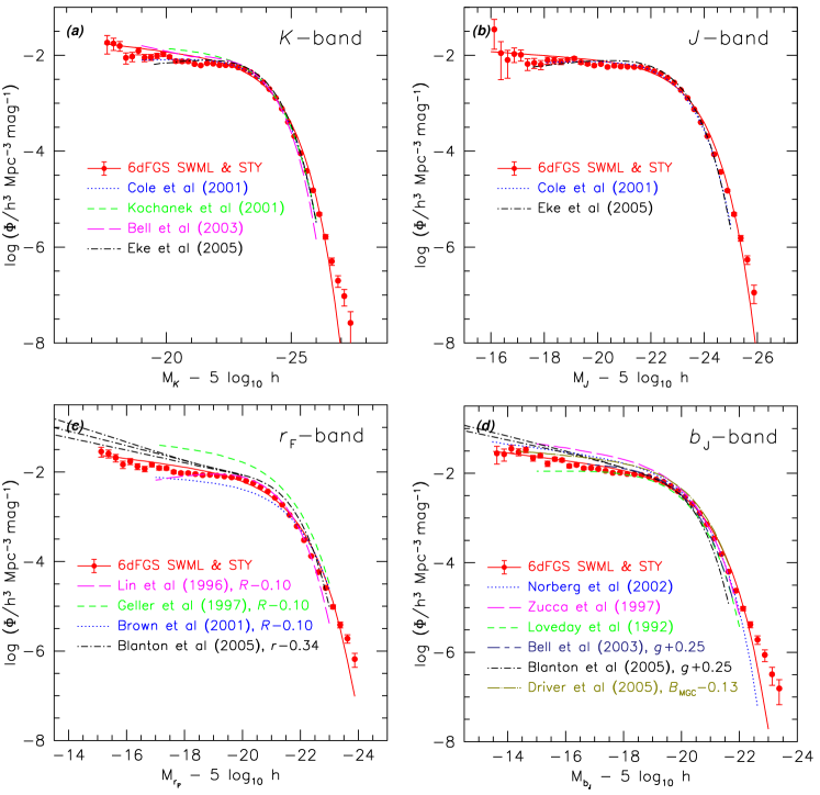
Figure 14 shows that the 6dFGS faint end slope ($\mbox{$\alpha$}=-1.21$) is closest to that of 2dFGRS and ESP, although the 6dFGS normalisation is lower than the others, possibly due to our non-use of evolution corrections (which are most significant in bluer passbands). These magnitude corrections (e.g. Norberg et al.; Bell et al.) tend to lower the bright end end relative to the faint end, and Blanton et al. has demonstrated $\sim 20$ to 30 percent variations are possible depending on the strength of the applied correction. We note that the 6dFGS normalisation ($\log\mbox{$\phi_{*}$}=-1.983$) most closely matches that of the Blanton et al. SDSS sample ($\log\mbox{$\phi_{*}$}=-1.928$), which (like the 6dFGS) was not corrected for evolution. We do not find evidence for the steep faint end upturn found by Blanton et al., despite having sufficient luminosity coverage to test for it. We suspect a local overdensity is the likely culprit for this feature of their data. Ultimately, subtle differences are inevitable because of the way deeper but narrower surveys (SDSS, 2dFGRS, ESP) sample the very nearest large-scale structures compared to the shallower but wider surveys such as Stromlo-APM and the 6dFGS.

5 Luminosity Density

The total luminosity per unit volume, or luminosity density, $j$, is a definitive observable of any galaxy population. It is the integral of the luminosity function, weighted by luminosity, and is given in solar luminosity units by

$$j=\mbox{$\phi_{*}$}\cdot 10^{-0.4(M_{*}-M_{\odot})}\cdot\Gamma(\mbox{$\alpha$}+2).$$ (11)

Figure 15 shows the luminosity densities calculated from Eqn. (11) and the 6dFGS STY fit parameters in Table 4. We have used solar absolute magnitudes of $M_{\odot}=(5.442,4.447,3.660,3.319,3.280)$ for $b_{\rm\scriptscriptstyle J}r_{\rm\scriptscriptstyle F}JHK$ respectively, made available by C. Willmer. We note that in the similar plot of Bell et al. (2003) (their Fig. 15) the $b_{\rm\scriptscriptstyle J}$ point for Norberg et al. (2002) is located $\sim 700$ Å blueward of its true value.

Figure 15: Integrated luminosity density for 6dFGS across $b_{\rm\scriptscriptstyle J}r_{\rm\scriptscriptstyle F}JHK$ in units of $10^{8}\,L_{\odot}\,h$ Mpc^-3 (large red solid circles, solid red line). Comparitive values from other recent surveys are also shown. Both $K$ values of Bell et al. (2003) are included: one with and one without correction for low surface brightness selection effects. We have also reproduced the spectral energy distribution of Bell et al. (2003) for a 12 Gyr old stellar population with exponentially decreasing star formation rate, with $e$-folding time of 4 Gyr (small solid circles, dashed line).

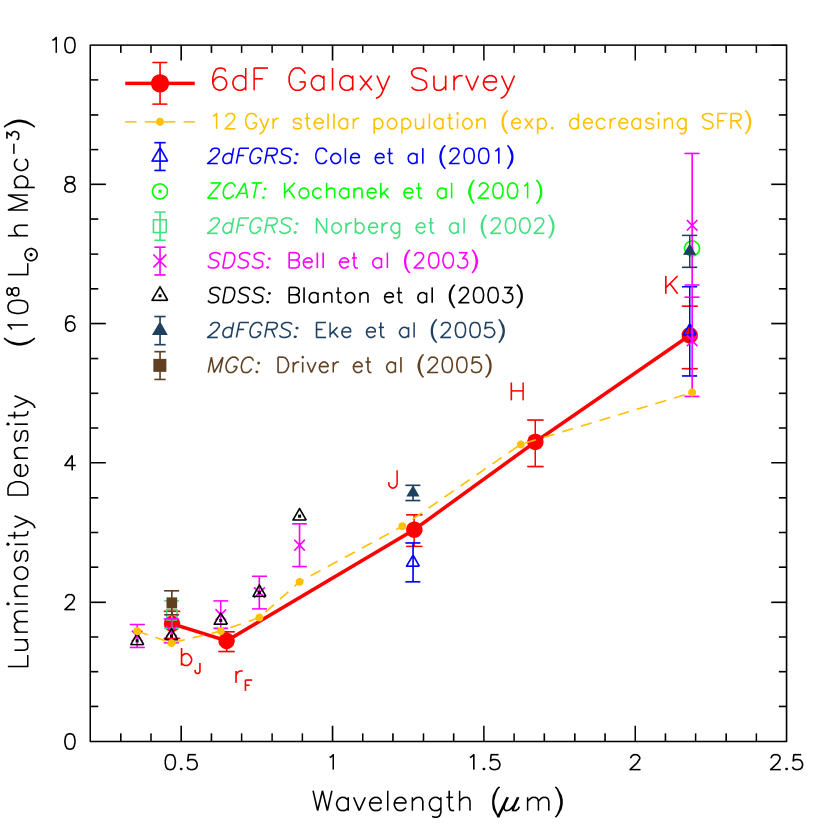
Figure 15 also shows how the luminosity densities from 6dFGS compare to those of other recent surveys. Although much has been made (see e.g. Wright, 2001; Norberg et al., 2002), of $\sim 2\times$ discrepancies between the early SDSS optical estimates (Blanton et al., 2001) and 2dFGRS in the NIR (, Cole et al.2001), the revised SDSS values of Blanton et al. (2003), corrected for cosmological evolution, have largely ameliorated these differences. The 6dFGS values agree with most recent estimates, finding a $K$-band value at the lower end of recent results for this band. This is also the expectation of the spectral energy distribution (SED) for a 12 Gyr old stellar population with a 4 Gyr $e$-folding exponentially decreasing star formation rate, (dashed line; after Bell et al., 2003). Models with more rapidly declining star formation rates ($\sim 2$ Gyr) can produce SEDs more luminous in $K$, but at the expense of overestimating optical luminosities by factors of $\sim 2$ or more.

While the luminosity density is a convenient quantity through which to compare different surveys and infer a volume-averaged SED, it ultimately relies on a fit to the LF and its extrapolation beyond accessible luminosities. We find that the STY fits consistently overestimate the integrated luminosity of the SWML method by $\sim 1$ to 3 percent across the observable range. The observed luminosity distribution typically accounts for around 95 percent of total luminosity, with the shortfall due almost entirely to faint-end extrapolation. This is comparable in size to the extra 2 to 5 percent integrated luminosity measured by the 6dFGS in reaching $\sim 1$ to 2 mags fainter in the NIR passbands.

6 Summary

We have presented luminosity functions in $KHJr_{\rm\scriptscriptstyle F}b_{\rm\scriptscriptstyle J}$ from the 6dF Galaxy Survey and derived luminosity densities from them. The 6dFGS target samples are drawn from the 2MASS XSC and SuperCOSMOS catalogues and are near-complete to limits of $(\mbox{$K$},\mbox{$H$},\mbox{$J$},\mbox{$r_{\rm\scriptscriptstyle F}$},\mbox{$b_{\rm\scriptscriptstyle J}$})=(12.75,13.00,13.75,15.60,16.75)$. The samples used here represent around half the final 6dFGS in terms of sky coverage and sample size. The 6dFGS is already the largest NIR-selected redshift survey by more than an order of magnitude in both coverage and sample size. Compared to the SDSS and 2dFGRS optical LFs it has around four times the sky coverage and half the sample size.

The 6dFGS luminosity functions have been calculated using the $1/V_{\rm max}$, STY and SWML estimators. The effects of magnitude and field-related incompleteness have been characterised and taken into account. Luminosity distances have been corrected for the effects of peculiar velocity, which can amount to differences as large as $\sim\pm 0.5$ mag for some supercluster members. The influence of photometric errors on the shape of the LF has been taken into account for $K$$H$$r_{\rm\scriptscriptstyle F}$$b_{\rm\scriptscriptstyle J}$, but was of little consequence for $J$.

These new 6dFGS LFs probe $\sim 1$ to 2 mag fainter in absolute magnitude than previous surveys in the NIR passbands and to comparable limits in $r_{\rm\scriptscriptstyle F}$ and $b_{\rm\scriptscriptstyle J}$. We obtain excellent agreement between the $1/V_{\rm max}$ and SWML estimates of the LFs, but find that a Schechter function (fitted by the optimal STY method) either under- or over-estimates these values by as much as 15 to 40 percent. While the formal uncertainties on our STY fits are typically a few percent or less in $\log\mbox{$\phi_{*}$}$, $M_{*}$ and $\alpha$, we show that, in comparison to the observed LF, a Schechter function is unable to decline rapidly enough at the bright-end and remain as flat at the faint end.

The 6dFGS results are generally in excellent agreement with other recent LF determinations in the NIR. We do not find as steep a faint-end slope as Kochanek et al. (2001), and suspect this is due to their shallower depth and subsequent brighter faint-end limit. The 6dFGS $r_{\rm\scriptscriptstyle F}$-band LF most closely matches those of the Las Campanas Redshift Survey (Lin et al., 1996) and SDSS (Blanton et al., 2005), although we find only marginal evidence for the faint-end upturn claimed by Blanton et al. In $b_{\rm\scriptscriptstyle J}$, the 6dFGS LF has a nearly identical faint end slope to those obtained by 2dFGRS (Norberg et al., 2002) and the ESO Slice Project (Zucca et al., 1997), although the 6dFGS normalisation is closer to that found by Blanton et al.. Neither this survey nor 6dFGS used evolutionary corrections. Furthermore, we see no evidence for a faint-end up-turn in any of the 6dFGS LFs.

The luminosity densities derived in all five 6dFGS passbands concur with most other recent measurements, and support a $K$-band value at the lower range of recent values. This is consistent with the effective mean galaxy spectral energy distribution being represented by an old stellar population with moderately decreasing star formation rate.

References

- (1) Abazajian, K., et al., (SDSS team), 2003, AJ, 126, 2081
- Andreon (2002) Andreon, S., 2002, A&A, 382, 495
- Baldry et al. (2005) Baldry I. K., et al., (SDSS team), 2005, MNRAS, 358, 441
- Bell & de Jong (2001) Bell, E. F., de Jong, R. S., 2001, ApJ, 550, 212
- Bell et al. (2003) Bell, E. F., McIntosh, D. H., Katz, N., Weinberg, M. D., 2003, ApJS, 149, 289
- Benson et al. (2003) Benson, A. J., Bower, R. G., Frenk, C. S., Lacey, C. G., Baugh, C. M., Cole, S., 2003, ApJ, 599, 38
- Berlind & Weinberg (2002) Berlind, A. A., Weinberg, D. H., 2002, ApJ, 575, 587
- Berlind et al. (2005) Berlind A. A., Blanton M. R., Hogg D. W., Weinberg D. H., Davé R., Eisenstein D. J., Katz N., 2005, ApJ, 629, 625
- Blanton et al. (2001) Blanton, M. R., et al., (SDSS team), 2001, AJ, 121, 2358
- Blanton et al. (2003) Blanton, M. R., et al., (SDSS team), 2003, ApJ, 592, 819
- Blanton et al. (2005) Blanton, M. R., Lupton, R. H., Schlegel, D. J., Strauss, M. A., Brinkmann, J., Fukugita, M., Loveday, J., 2005, ApJ, 631, 208
- Brown et al. (2001) Brown, W. R., Geller, M. J., Fabricant, D. G., Kurtz, M. J., 2001, AJ, 122, 714
- Burstein et al. (1989) Burstein, D., Davies, R. L., Dressler, A., Faber, S. M., Lynden-Bell, D., 1989, in Large Scale Structure and Motions in the Universe; Proceedings of the International Meeting, Trieste, Italy, Apr. 6-9, 1988, ed. by Mezzetti, M.; Dordrecht, Kluwer Academic Publishers, 1989, p. 179-194
- (14) Cole, S. et al., (2dFGRS team), 2001, MNRAS, 326, 255
- Cole et al. (2005) Cole, S., et al., (2dFGRS team), 2005, MNRAS, 362, 505
- Colless et al. (2001) Colless, M. et al., (2dFGRS team), 2001, MNRAS, 328, 1039
- (17) Cooray, A., Milosavljević, M., 2005, ApJ, 627, L89
- Cross et al. (2001) Cross, N., et al., (2dFGRS team), 2001, MNRAS, 324, 825
- Cross & Driver (2002) Cross, N., Driver, S. P., 2002, MNRAS, 329, 579
- Cross et al. (2004) Cross, N. J. G., et al., (2dFGRS team), 2004, MNRAS, 349, 576
- Croton et al. (2005) Croton D. J., et al., (2dFGRS team), 2005, MNRAS, 356, 1155
- Dalcanton (1998) Dalcanton, J. J., 1998, ApJ, 495, 251
- de Jong & Lacey (2000) de Jong, R. S., Lacey, C., 2000, ApJ, 545, 781
- De Propris et al. (2003) De Propris R., et al., (2dFGRS team), 2003, MNRAS, 342, 725
- Disney (1976) Disney, M. J., 1976, Nature, 263, 573
- Driver (1999) Driver, S. P., 1999, ApJ, 526, L69
- Driver (2004) Driver, S., 2004, PASA, 21, 344
- Driver et al. (2005) Driver, S. P., Liske, J., Cross, N. J. G., De Propris, R., Allen, P. D., 2005, MNRAS, 360, 81
- Efstathiou, Ellis & Peterson (1988) Efstathiou, G., Ellis, R. S., Peterson, B. A., 1988, MNRAS, 232, 431
- Eke et al. (2004) Eke V. R., et al., (2dFGRS team), 2004, MNRAS, 355, 769
- Eke et al. (2005) Eke, V. R., Baugh, C. M., Cole, S., Frenk, C. S., King, H. M., Peacock, J. A., 2005, MNRAS, 362, 1233
- Felten (1976) Felten, J. E., 1976, ApJ, 207, 700
- Folkes et al. (1999) Folkes S., et al., (2dFGRS team), 1999, MNRAS, 308, 459
- Fukugita, Shimasaku & Ichikawa (1995) Fukugita, M., Shimasaku, K., Ichikawa, T., 1995, PASP, 107, 945
- Geller et al. (1997) Geller, M. J., Kurtz, M. J., Wegner, G., Thorstensen, J. R., Fabricant, D. G., Marzke, R. O., Huchra, J. P., Schild, R. E., et al., 1997, AJ, 114, 2205
- Goto et al. (2002) Goto T., et al., (SDSS team), 2002, PASJ, 54, 515
- Hubble (1934) Hubble, E., 1934, ApJ, 79, 8
- Huchra et al. (1992) Huchra, J. P., et al., The Center for Astrophysic Redshift catalog (1992 version), 1992, Center for Astrophysics
- Huchra et al. (2006) Huchra, J. P., et al., 2006, in prep.
- Impey & Bothun (1997) Impey, C., Bothun, G., 1997, ARA&A, 35, 267
- Jarrett et al. (2000) Jarrett, T. H., Chester, T., Cutri, R., Schneider, S., Rosenberg, J., Huchra, J. P., Mader, J., 2000, AJ, 120, 298
- Jarrett et al. (2003) Jarrett, T. H., Chester, T., Cutri, R., Schneider, S. E., Huchra, J. P., 2003, AJ, 125, 525
- Jarrett (2004) Jarrett, T., 2004, PASA, 21, 396
- Jones et al. (2004) Jones, D. H., Saunders, W., Colless, M., Read, M. A., Parker, Q. A., Watson, F. G., Campbell, L. A., Burkey, D., et al., 2004, MNRAS, 355, 747
- Jones et al. (2005) Jones, D. H., Saunders, W., Read, M., Colless, M., 2005, PASA, 22, 277
- Kaldare (2001) Kaldare, R., 2001, PhD Thesis, Australian National University
- Kay et al. (2002) Kay, S. T., Pearce, F. R., Frenk, C. S., Jenkins, A., 2002, MNRAS, 330, 113
- Kochanek et al. (2001) Kochanek, C. S., Pahre, M. A., Falco, E. E., Huchra, J. P., Mader, J., Jarrett, T. H., Chester, T., Cutri, R., et al., 2001, ApJ, 560, 566
- Lin et al. (1996) Lin, H., Kirshner, R. P., Shectman, S. A., Landy, S. D., Oemler, A., Tucker, D. L., Schechter, P. L., 1996, ApJ, 464, 60
- Loveday et al. (1992) Loveday, J., Efstathiou, G., Peterson, B. A., Maddox, S. J., 1992, ApJ, 400, L43
- Loveday (2000) Loveday, J., 2000, MNRAS, 312, 557
- Madgwick et al. (2002) Madgwick D. S., et al., (2dFGRS team), 2002, MNRAS, 333, 133
- Mould et al. (2000) Mould, J. R., Huchra, J. P., Freedman, W. L., Kennicutt, R. C., Ferrarese, L., Ford, H. C., Gibson, B. K., Graham, J. A., et al., 2000, ApJ, 529, 786
- Murdoch, Crawford & Jauncey (1973) Murdoch, H. S., Crawford, D. F., Jauncey, D. L., 1973, ApJ, 183, 1
- Norberg et al. (2002) Norberg, P., et al., (2dFGRS team), 2002, MNRAS, 336, 907
- Phillipps, Davies & Disney (1990) Phillipps, S., Davies, J. I., Disney, M. J., 1990, MNRAS, 242, 235
- Poggianti (1997) Poggianti, B. M., 1997, A&AS, 122, 399
- Press & Schechter (1974) Press, W. H., Schechter, P., 1974, ApJ, 187, 425
- Rees & Ostriker (1977) Rees, M. J., Ostriker, J. P., 1977, MNRAS, 179, 541
- Sandage, Tammann & Yahil (1979) Sandage, A., Tammann, G. A., Yahil, A., 1979, ApJ, 232, 352
- Saunders et al. (1990) Saunders, W., Rowan-Robinson, M., Lawrence, A., Efstathiou, G., Kaiser, N., Ellis, R. S., Frenk, C. S. 1990, MNRAS, 242, 318
- Schechter (1976) Schechter, P., 1976, ApJ, 203, 297
- Schlegel, Finkbeiner & Davis (1998) Schlegel, D. J., Finkbeiner, D. P., Davis, M., 1998, ApJ, 500, 525
- Schmidt (1968) Schmidt, M., 1968, ApJ, 151, 393
- Sprayberry et al. (1997) Sprayberry, D., Impey, C. D., Irwin, M. J., Bothun, G. D., 1997, ApJ, 482, 104
- Stoughton et al. (2002) Stoughton, C., et al., (SDSS team), 2002, AJ, 123, 485
- Tonry et al. (2000) Tonry, J. L., Blakeslee, J. P., Ajhar, E. A., Dressler, A., 2000, ApJ, 530, 625
- Willmer (1997) Willmer, C. N. A., 1997, AJ, 114, 898
- Wright (2001) Wright, E. L., 2001, ApJ, 556, L17
- Yang, Mo & van den Bosch (2003) Yang, X., Mo, H. J., van den Bosch, F. C., 2003, MNRAS, 339, 1057
- Zucca et al. (1997) Zucca, E., Zamorani, G., Vettolani, G., Cappi, A., Merighi, R., Mignoli, M., Stirpe, G. M., MacGillivray, H., et al., 1997, A&A, 326, 477