Modelling galaxy clustering in a high resolution simulation of structure formation

Abstract

We use the Millennium Simulation, a 10 billion particle simulation of the growth of cosmic structure, to construct a new model of galaxy clustering. We adopt a methodology that falls midway between the traditional semi-analytic approach and the halo occupation distribution (HOD) approach. In our model, we adopt the positions and velocities of the galaxies that are predicted by following the orbits and merging histories of the substructures in the simulation. Rather than using star formation and feedback ‘recipes’ to specify the physical properties of the galaxies, we adopt parametrized functions to relate these properties to the quantity $M_{infall}$, defined as the mass of the halo at the epoch when the galaxy was last the central dominant object in its own halo. We test whether these parametrized relations allow us to recover the basic statistical properties of galaxies in the semi-analytic catalogues, including the luminosity function, the stellar mass function and the shape and amplitude of the two-point correlation function evaluated in different stellar mass and luminosity ranges. We then use our model to interpret recent measurements of these quantities from Sloan Digital Sky Survey data. We derive relations between the luminosities and the stellar masses of galaxies in the local Universe and their host halo masses. Our results are in excellent agreement with recent determinations of these relations by Mandelbaum et al using galaxy-galaxy weak lensing measurements from the SDSS.

1 Introduction

According to the current standard paradigm, galaxies form and reside inside extended dark matter haloes. Three different approaches have been used to model the link between the properties of galaxies and the dark matter haloes in which they are found. One approach is to carry out N-body + hydrodynamical simulations that include both gas and dark matter(Katz et al., 1996; Pearce et al., 2001; White et al., 2001; Yoshikawa et al., 2001). Another approach is to combine N-body simulations with simple prescriptions, taken directly from semi-analytic models of galaxy formation(Kauffmann et al., 1999), to track gas cooling and star formation in galaxies. The third method is the so called Halo Occupation Distribution (HOD) approach, which aims to provide a purely statistical description of how dark matter haloes are populated by galaxies.

Typical HOD models are constructed by specifying the number of galaxies $N$ that populate a dark matter halo of mass $M$ as well as the distribution of galaxies within these haloes(Kauffmann et al., 1997; Peacock & Smith, 2000; Seljak, 2000; Benson et al., 2000; Berlind & Weinberg, 2002; Berlind et al., 2003). More recent models have concentrated on the so-called conditional luminosity function $\Phi(L|M)dL$, which gives the number of galaxies of luminosity $L$ that reside in a halo of mass $M$(Yang et al., 2003). Most HOD models also distinguish between “central” galaxies, located at the centres of dark matter haloes and “satellite” galaxies, which are usually assumed to have the same density profile as the dark matter within the halo. Physically, this is supposed to reflect the fact that gas cools and accumulates at the halo centres until the halo merges with a larger structure. With this approach, the models can be used to explore the parameters that are required to match simultaneously the galaxy luminosity function as well as the the luminosity, colour and morphology dependences of the correlation function(van den Bosch et al., 2003; Zehavi et al., 2005; Yang et al., 2005). Other papers have used HOD models to explore the detailed shape of two-point correlation function(Zehavi et al., 2004) as well as higher order correlation functions(Wang et al., 2004).

N-body simulations can now be carried out with high enough resolution to track the histories of individual substructures (subhaloes) within the surrounding halo(Springel et al., 2001). It is thus becomes possible to specify the positions and velocities of galaxies within a halo in a dynamically consistent way, rather than assuming a profile or form for the velocity distribution. Galaxy clustering statistics that are computed using the full information available from these high resolution simulations should in principle be more accurate and robust.

Caution must be exercised, however, when only using subhaloes as tracers of galaxies in high resolution simulations, as has been recently done by Vale & Ostriker (2004, 2005); Conroy et al. (2005). In standard models of galaxy formation, when a galaxy is accreted by a larger system such as a cluster, its surrounding gas is shock–heated to high temperatures. Star formation then terminates as the internal gas supply of the galaxy is used up. The stellar masses of satellite galaxies only change by a small amount after they are accreted, while their luminosities dim due to aging of their stars. In contrast, the dark matter haloes surrounding the satellites gradually lose mass as their outer regions are tidally stripped (De Lucia et al., 2004). Near the centres of the halos, most of the substructures have been completely destroyed. Gao et al. (2004) have shown that the radial distribution of subhaloes is much less centrally concentrated than the radial distribution of galaxies predicted by simulations that follow the full orbital and merging histories of these systems.

In this paper, we make use of the Millennium Simulation, a 10 billion particle simulation of the growth of cosmic structure, to construct a new model of galaxy clustering. We adopt a methodology that falls in between the semi-analytic approach, which tracks galaxy formation ‘ab initio’ within the simulation, and the HOD approach, which only provides a statistical description of how galaxies are related to the underlying dark matter density distribution. In our approach, we adopt the positions and velocities of the galaxies as predicted by following the orbits and merging histories of the substructures in the simulation. Rather than using star formation and feedback ‘recipes’ to calculate how the physical properties of the galaxies such as their luminosities or stellar masses evolve with time, we adopt parametrized functions to relate these properties to the quantity $M_{infall}$, defined as the mass of the halo at the epoch when the galaxy was last the central dominant object. For central galaxies at the present day, $M_{infall}$ is simply the present day halo mass, but for satellite galaxies, it is the mass of the halo when the galaxy was first accreted by a larger structure.

This approach has the advantage of the semi-analytic models in that it provides very accurate positions and velocities for all the galaxies in the simulation. It maintains the simplicity of the HOD approach, because it bypasses the need to incorporate detailed treatment of star formation and feedback processes. Our aim in developing these models is to use them as a means of constraining the relation between galaxy physical properties and halo mass directly from observational data, not as a means of understanding the physics of galaxy formation.

The paper is organized as follow: we first introduce the Millennium Run and the methodology used for identifying haloes, subhaloes and galaxies in this simulation. We then study the relation between luminosity/stellar mass and $M_{infall}$ in mock galaxy catalogues constructed using these simulations. In Sec. 4 we introduce a parametrization for these relations and show that we are able to recover basic statistical quantities such as the galaxy luminosity/mass function and the shape and amplitude of the two-point correlation function in different luminosity/mass bins. We also investigate the the effect of changing the parameters of the relation on the luminosity function and correlation function. In Sec. 5 we apply the method to real data on the clustering of galaxies as a function of luminosity and stellar mass(Li et al., 2006) derived from the Sloan Digital Sky Survey (SDSS). Finally, we discuss our results and present our conclusions.

Figure 1: Relations between stellar mass, baryonic mass and $M_{infall}$ calculated from the semi-analytic galaxy catalogues. Open circles represent central galaxies and triangles are for satellite galaxies. Error bars indicate the $95$ percentiles of the mass distribution at the given value of $M_{infall}$. Dashed lines show the double power law parametrized fit to the median value of relations for the galaxy sample as whole.

2 The Simulation

The Millennium Simulation(Springel et al., 2005) used in this study, is the largest simulation of cosmic structure growth carried out so far. The cosmological parameters values in the simulation are consistent with recent determinations from a combined analysis of the 2dFGRS(Colless et al., 2001) and first year WMAP data (Spergel et al., 2003). A flat $\Lambda$CDM cosmology is assumed with $\Omega_{\rm m}=0.25$, $\Omega_{\rm b}=0.045$, $h=0.73$, $\Omega_{\Lambda}=0.75$, $n=1$, and $\sigma_{8}=0.9$. The simulation follows $N=2160^{3}$ particles of mass $8.6\times 10^{8}\,h^{-1}{\rm M}_{\odot}$ from redshift $z=127$ to the present day, within a comoving box of $500\,h^{-1}$Mpc on a side.

Full particle data are stored at 64 output times. For each output, haloes are identified using a friends-of-friends (FOF) group-finder. Substructures (or subhaloes) within a FOF halo are located using the SUBFIND algorithm of Springel et al. (2001). After finding all haloes and subhaloes at all output snapshots, merging trees are built describing in detail how these systems merge and grow as the universe evolves. Since structures merge hierarchically in CDM universes, for any given halo, there can be several progenitors, but in general each halo or subhalo only has one descendant. Merger trees are thus constructed by defining a unique descendant for each halo and subhalo. Through those merging trees, we are able to follow the history of haloes/subhaloes, as well as the galaxies inside them.

Once a halo appears in the simulation, it is assumed that a galaxy begins to form within it. As the simulation evolves, the halo may merge with a larger structure and become a subhalo, while the galaxy becomes a satellite galaxy. The galaxy’s position and velocity are specified by the position and velocity of the most bound particle of its host halo/subhalo. Even if the subhalo hosting the galaxy is tidally disrupted, the position and velocity of the galaxy is still traced through this most bound particle. We will refer to these galaxies without subhaloes as “orphaned” systems. Galaxies thus only disappear from the simulation if they merge with another galaxy. The time taken for an orphaned galaxy to merge with the central object is given by the time taken for dynamical friction to erode its orbit, causing it to spiral into the centre and merge. The satellite orbits are thus tracked directly until the subhalo is disrupted; thereafter, the time taken for the galaxy to reach the centre is calculated using the standard Chandrasekhar formula.

In this paper, we will parameterize quantities such as galaxy luminosity and stellar mass as a function of the quantity $M_{infall}$, which is defined as the virial mass of the halo hosting the galaxy at the epoch when it was last the central galaxy of its own halo. The Millennium simulation catalogues include haloes down to a resolution limit of 20 particles, which yields a minimum halo mass of $2\times 10^{10}h^{-1}M\odot$. In our study, we only consider galaxies with $M_{infall}$ greater than $10^{10.5}h^{-1}M\odot$.(Note that $M_{infall}$ is simply the virial mass of the host halo for central galaxies at the present day.) This results in a total sample of $11761178$ galaxies within the simulation volume.

3 The relations between M_infall, stellar mass and luminosity in the semi-analytic galaxy catalogues

In the following two sections we use the semi-analytic galaxy catalogues constructed from the Millennium simulation by (Croton et al., 2006) (http://www.mpa-garching.mpg.de/galform/agnpaper/) to study how galaxy properties such as stellar mass, baryonic mass (i.e. stellar mass+ cold gas mass) and luminosity depend on $M_{infall}$, the mass of the halo in which the galaxy was last a central object. We construct parametrized relations between these quantities and $M_{infall}$ that match the relations found in the mock catalogue. We then show that our parametrization allows us to recover both the luminosity/mass functions of the simulated galaxies and the shape, amplitude and mass/luminosity dependence of the two-point correlation functions. Croton et al. (2006) have shown that their catalogues provide a good match to the observed galaxy luminosity function and the clustering properties of galaxies, so we believe that it is a reasonable to use these catalogues as a way of motivating and testing our simple parametrizations.

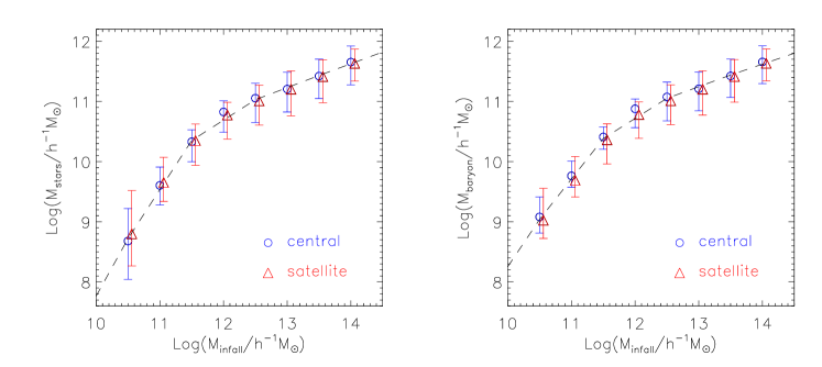
In Fig. 1 we plot the relations between $M_{infall}$ and galaxy stellar mass ($M_{stars}$) and baryonic mass ($M_{baryon}$). We show results for present-day central galaxies in blue and satellite galaxies in red. Error bars indicate the 95th percentiles of the distributions. As we will show, the relations between $M_{infall}$ and $M_{stars}$/ $M_{baryon}$ are well described by a double power law. The crossover point between the two power laws is at a halo mass of $\sim 3\times 10^{11}h^{-1}M_{\odot}$, which corresponds to a galaxy with stellar mass of around $10^{10}h^{-1}M_{\odot}$. In less massive haloes, supernova feedback acts to prevent gas from cooling and forming stars as efficiently as in high mass haloes. In massive haloes, the cooling times become longer and a smaller fraction of the baryons are predicted to cool and form stars. In addition, in the models of Croton et al. (2006), heating from AGN also acts to suppress cooling onto high mass galaxies.

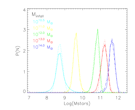
Fig. 2 shows that the distribution of $M_{stars}$ at a given value of $M_{infall}$ is well-described by a log-normal function. The width of the lognormal depends weakly on halo mass with a maximum dispersion $\sigma$ of 0.2 dex at $M_{infall}=10^{10.5}h^{-1}M_{\odot}$ and a minimum $\sigma$ of 0.1 dex at $M_{infall}=10^{11.5}h^{-1}M_{\odot}$. The relations depend very little on whether the galaxy is a central or satellite system. The dispersion around the relations is also similar for the two types(in Fig. 2, the solid and dashed lines for central and satellite galaxies lie almost on top of each other). The similarity in the $M_{infall}$- $M_{stars}$ relations between satellite and centrals may be regarded as something of a coincidence. Although there is little change in the stellar/baryonic component of the galaxy after it falls into a larger structure, halos of the same mass at different times have different circular velocities and hence different cooling and and star formation efficiencies. As we will show later, we obtain better fits to the observational data if we allow the relations between central and satellites galaxies to differ.

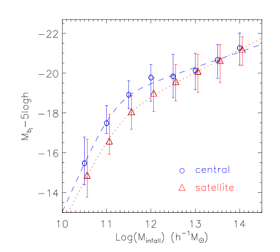
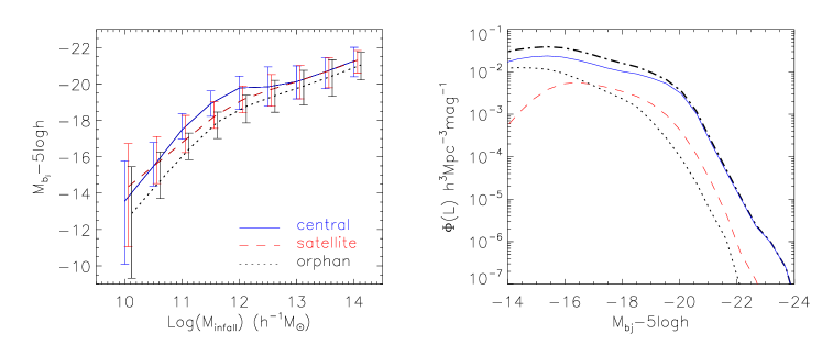
Fig. 3 shows the relation between luminosity and $M_{infall}$. It also can be fit by a double power law, but the difference between central and satellite galaxies is much more obvious. At a given value of $M_{infall}$ central galaxies are more luminous than satellites because they are forming stars at higher rates and their stellar mass-to-light ratios are lower. The difference between central and satellite galaxies becomes very small at large values of $M_{infall}$. This can be understood as a simple consequence of hierarchical structure formation: massive haloes were formed more recently than less massive haloes and subhaloes with large masses are likely to have been accreted relatively recently. Massive satellite galaxies have therefore not been satellites for long and thus have mass-to-light ratios that are more similar to their central counterparts. In addition the Croton et al models include a “radio AGN mode” of feedback, which acts to suppress cooling onto the most massive galaxies. This also acts to reduce the difference between central and satellite galaxy colours and mass-to-light ratios.

Figure 2: The distribution in stellar mass for different $M_{infall}$ bins increasing from $10^{10.5}h^{-1}M\odot$(left) to $10^{14.0}h^{-1}M\odot$(right). Solid and dashed lines are for central and satellite galaxies (note that they lie on top of each other for three lower mass bins). Dotted lines indicate the Gaussian fits to the distributions that are used in our parametrized model.

Figure 3: The same as in Fig. 1, but luminosity (represented by magnitude of $b_{j}$ band) is plotted as a function of $M_{infall}$. Dashed(dotted) lines show the double power law fits to the relation for central(satellite) galaxies.

4 Parametrizations and tests

Table 1: Best-fit parameter values for the relations between $M_{infall}$ and $M_{stars}$, $M_{baryon}$ and $L$ as derived from the semi-analytic galaxy catalogues of Croton et al. (2006).

		$M_{0}(h^{-1}M_{\odot})$	$\alpha$	$\beta$	$log(k)$	$\sigma$	$\tilde{\chi}^{2}$
$M_{stars}$	total	3.16$\times 10^{11}$	0.39	1.92	10.35	0.156	0.0146
	central	3.16$\times 10^{11}$	0.39	1.96	10.35	0.148	0.0240
	satellite	3.16$\times 10^{11}$	0.39	1.83	10.34	0.167	0.0057
$M_{baryon}$	total	3.61$\times 10^{11}$	0.36	1.59	10.44	0.147	0.0415
	central	3.61$\times 10^{11}$	0.35	1.59	10.46	0.133	0.0542
	satellite	3.61$\times 10^{11}$	0.37	1.59	10.40	0.162	0.0273
$L(M_{bj})$	total	1.49$\times 10^{11}$	0.36	1.90	7.14	0.215	0.0360
	central	1.49$\times 10^{11}$	0.31	1.99	7.25	0.169	0.1250
	satellite	1.49$\times 10^{11}$	0.46	1.81	6.90	0.189	0.0359

4.1 Functional form

We use a two–power–law model of the following form to fit the median value of the relations between $M_{stars}$, $M_{baryon}$, $L$ and $M_{infall}$:

$${x}=\frac{2}{(\frac{{M}_{infall}}{{{M}_{0}}})^{-\alpha}+(\frac{{M}_{infall}}{{{M}_{0}}})^{-\beta}}{\times}{k},$$

where $x$ denotes $M_{stars}$,$M_{baryon}$ or $L$, and the relation between luminosity $L$ and $b_{j}$ band magnitude is given by:

$${{M}_{b_{j}}-{5}{\log}{h}}={-2.5}{\log}{L}$$

We fit these relations for central and satellite galaxies separately, as well as for the galaxy population as a whole. We will later test whether separate fits to the central galaxies and satellites make significant difference to our results. We also assume that the dispersion around the median value has a lognormal form.

Table 1 lists the parameters of the best–fitting models for the relations between $M_{infall}$ and $M_{stars}$, $M_{baryon}$ and $L$. The models have five parameters.

1. $M_{0}$ is the critical mass/luminosity at which the slope of the relation changes. When we fit satellite and central galaxies separately, we find almost exactly the same values for this parameter (even for luminosity, the difference is less than 20%). We therefore fix $M_{0}$ at the best-fit value for the galaxy sample as a whole.

2. $\alpha$ and $\beta$ describe the slope of the relations at high and low values of $M_{infall}$.

3. $k$ is a normalization constant.

4. We have calculated the interval in $\log M_{stars}$, $\log M_{baryon}$ and $\log L$ that encloses the central 68% of the probability distribution for 8 different values of $\log M_{infall}$ from $10^{10.5}h^{-1}M\odot$ to $10^{14}h^{-1}M\odot$, with step 0.5 dex. We then calculate the average of these 8 values and the value of $\sigma$ quoted in Table 1 is 0.5 times this number.

The resulting model fits are plotted as dashed and dotted lines in Fig. 1 and Fig. 3. The quality of the fit is given in the last column of Table 1 and is calculated as:

$${\tilde{\chi}^{2}}=\sum{(\frac{{x_{fit}}-{x_{SAM}}}{{x_{SAM}}})^{2}}$$

where $x$ represents $M_{stars}$, $M_{baryon}$, $L$ for each relation, and the sum is over the $8$ mass bins with $10^{10.5}h^{-1}M_{\odot}{\leq}M_{infall}\leq 10^{14.0}h^{-1}M_{\odot}$.

Figure 4: Results from the comparison of the parametrized model and the semi-analytic galaxy catalogue. The left panel shows the stellar mass function. The right panel shows correlation functions for three different stellar mass bins: $10^{9}h^{-1}M\odot$, $10^{10.5}h^{-1}M\odot$ and $10^{11.5}h^{-1}M\odot$. Symbols are for the semi–analytic galaxy catalogue. Solid lines are for our parametrized models.

Figure 5: Same as Fig. 4, except for the luminosity function (left) and the correlation function as a function of absolute magnitude (right). Symbols are the semi-analytic results, error bars in the right panel are the boot strap error of correlation length for the semi-analytic model. Solid lines are for parametrized models where relations for central galaxies and satellite galaxies are fit separately. The dashed lines are for models where the fit is for the galaxy population as a whole.

4.2 Tests

The next step is to see whether these parametrized relations allow us to recover the basic statistical properties of the simulated galaxy catalogue, such as the mass/luminosity function and the mass/luminosity dependence of the two point correlation function. When fitting to the quantities $M_{star}$ and $M_{baryon}$, we do not distinguish between central and satellite galaxies because the relations are almost the same for both. When fitting to galaxy luminosity, we do allow $\alpha$, $\beta$, $k$ and $\sigma$ to vary between central and satellite galaxies, but $M_{0}$ remains fixed for both. Note that the positions and the velocities of the galaxies are exactly the same as specified in the semi-analytic galaxy catalogues; the parametrized relations between galaxy mass/luminosity and $M_{infall}$ simply provide us with a alternative way of specifying the properties of the galaxies.

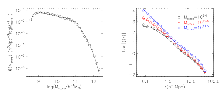
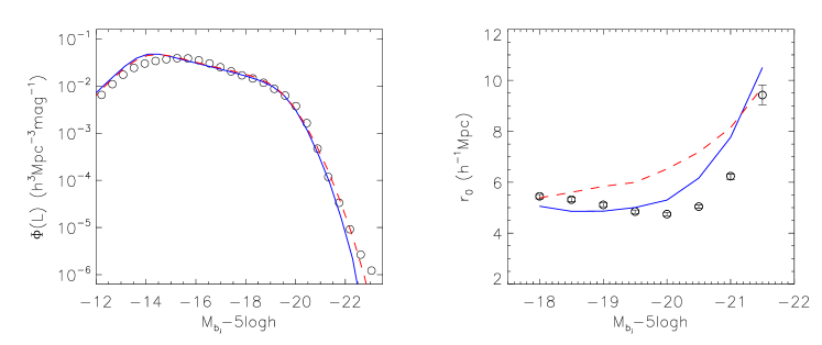
Fig. 4 and Fig. 5 show the results of our test. Symbols show results calculated directly from the semi-analytic galaxy catalogues and lines are from our parametrized model. The stellar mass function is well reproduced, and we can also recover the correlation for different stellar mass bins: $10^{9}h^{-1}M_{\odot}$, $10^{10.5}h^{-1}M_{\odot}$ and $10^{11.5}h^{-1}M_{\odot}$(Fig. 4). For luminosity, the parametrized model is not quite as successful. Although the luminosity function is well-reproduced, there are some discrepancies in the dependence of the clustering amplitude on luminosity (solid-blue curve in Fig. 5). Part of the reason for this discrepancy is that our parametrization of the $L-M_{infall}$ relation has somewhat larger $\chi^{2}$ than the $M_{stars}-M_{infall}$ relation (see Table.1). In addition, in order to reproduce the clustering trends as a function of luminosity, it is critical to fit the relation for central and for satellites galaxies separately. If we apply a single relation for both kinds of galaxies, we obtain the red-dashed curve in Fig. 5, which is even more discrepant. Our results suggest that in order to reproduce the clustering dependence on luminosity in a more exact way, one would need to introduce an additional dependence of the $L-M_{infall}$ relation on the parameter $t_{infall}$, the time when the galaxy was last the central object of its own halo. This does not appear to be necessary in order to reproduce the stellar mass dependence of galaxy clustering. The reason for this difference is because the optical light from galaxies, unlike their stellar mass, is heavily influenced by the contribution from the youngest stars, which have lifetimes which are short compared to the age of the Universe. Once a galaxy becomes a satellite, it will fade in luminosity even though its stellar mass remains approximately constant. For the sake of simplicity, we will not introduce $t_{infall}$ as an additional parameter in this paper, but we will come back to this in future work in which we consider the colour-dependence of galaxy clustering.

Figure 6: $L-M_{infall}$ relations(left) and luminosity functions(right) for different types of galaxies from the semi-analytic galaxy catalogue: central galaxies (solid lines), satellite galaxies with subhaloes (dashed lines), satellite galaxies without subhaloes (dotted lines). The dashed-dotted line in the right-hand panel shows the total luminosity function for all galaxies.

Figure 7: Correlation functions for three luminosity bins including (solid lines) and not including (dashed lines) orphan satellite galaxies.

4.3 The effect of “Orphan” Galaxies

The majority of HOD models in the literature only consider dark matter haloes and subhaloes that can be identified at the present time. Satellite galaxies without surrounding subhaloes are thus omitted from the analysis. We now explore the effect of these ’orphan’ satellite galaxies on our results.

The left panel of Fig. 6 compares the $L-M_{infall}$ relation for orphan satellites with the results obtained for central galaxies and satellite galaxies that have retained their subhaloes. The right panel of Fig. 6 shows the relative contribution of central galaxies, satellite galaxies with subhaloes and orphan satellites without subhaloes to the luminosity function of the galaxies in the semi-analytic catalogue. As can be seen, orphan satellites have lower luminosities at a given value of $M_{infall}$ than either central galaxies or satellite galaxies with subhaloes – i.e. orphan galaxies are the oldest galaxies with the highest mass-to-light ratios in the simulation. In addition, we see that the contribution of these orphan satellites is highest at the faintest lumninosities. Fig. 7 explores the contribution of the orphan satellites to the correlation function in three different bins of absolute magnitude. The solid curves show the result for all the galaxies while the dashed red curves show the result when the orphan satellites are omitted. As can be seen, the orphaned satellites contribute heavily to the correlation function of faint galaxies on scales of less than 1 Mpc. Omission of these systems causes the amplitude of the correlation function to be underestimated by more than an order of magnitude at separations of 0.1 Mpc for galaxies with $-18<M_{bj}<-17$.

We note that there are uncertainties in our treatment of orphan galaxies in the simulation. Some of these galaxies may indeed be destroyed or significantly reduced in mass by tidal stripping effects. Indeed, the existence of a significant intra-cluster light component does suggest tidal effects or mergers do unbind some of the stars in satellite galaxies(Arnaboldi, 2004; Feldmeier et al., 2004; Zibetti et al., 2005). In face of these uncertainties, we have chosen to assume that the visible galaxies survive even after their subhalo falls below the resolution limit of the simulation. It is possible that we over-estimate the number of these objects because we do not include tidal stripping on the stellar component. However, we believe that ”orphan” galaxies (at least part of them) are needed in order to explain observational results. From Fig.7 we see that when ”orphan” galaxies are excluded, the correlation signal decreases at small scales, at odds with observational results(see later in Fig.9 and Fig.10). In this work we consider all the ’orphan’ systems as part of satellite subsamples.

4.4 Changes in the input parameters

One advantage of our parametrized approach is that we can understand the effect of changing each different parameter and thus gain intuition about what changes are necessary to bring the models into the closest possible agreement with the observational data. This is different in spirit to exploring parameter space in the semi-analytic models, because the parameters in these models are tied to the physical recipes for star formation and feedback rather than the relation between halo mass and galaxy properties, which is the focus of our approach.

In the upper panel of Fig. 8, we show how changing each of the parameters affects the stellar mass function. Note that the normalization constant $k$ is always adjusted in order to keep the amplitude of the mass function at $M_{stars}=10^{11}M_{\odot}$ fixed. Changing $M_{0}$ affects the mass scale of the transition between the two power laws as well as the amplitude of the mass function at both low and at high masses. Changes to $\alpha$ affect the shape of the mass function at the high mass end, while changes to $\beta$ affect the low mass end of the mass function. A change in scatter $\sigma$ has similar effect to a change in $\alpha$, and influences the amplitude of the mass function at the high mass end. This is because the mass function is relatively flat at low masses and declines steeply at high masses, so an increasing amount of scatter in the $M_{stars}-M_{infall}$ relation will have a strong effect on the number of high mass galaxies.

The lower panels in Fig. 8 show the effect of the same parameter changes on the amplitude of the correlation function evaluated on scales of $r=0.33h^{-1}$ Mpc and $r=5.30h^{-1}$ Mpc. We see that a parameter change that causes an increase in the number of galaxies of given mass, will cause a corresponding decrease in the clustering amplitude of these systems. This is easy to understand. In order to have more galaxies of a given mass in the simulation, they must be shifted into lower mass haloes and these low mass haloes are more weakly clustered.

Figure 8: The effect of changing parameters on the stellar mass function(upper panels) and correlation at scales of $r=0.33h^{-1}Mpc$ and $r=5.30h^{-1}Mpc$(lower panels). The solid lines represent the best fit model for the $M_{stars}-M_{infall}$ relation.

5 Application to SDSS

In this section, we apply our models to observational data from the Sloan Digital Sky Survey. Recent large scale redshift surveys such as 2dfGRS(Colless et al., 2001) and Sloan Digital Sky Survey(SDSS; York et al. (2000)) provide galaxy samples that are large enough to measure the luminosity dependence of galaxy clustering accurately (Norberg et al., 2002a, b; Zehavi et al., 2005). In this paper, we make use of the recent measurements of the projected correlation function $w(r_{p})$ by Li et al. (2006). These authors calculated $w(r_{p})$ not only as a function of galaxy luminosity, but also stellar mass using a sample of galaxies constructed from the SDSS Data Release 2 (DR2) data. The methods for estimating the stellar masses are described in Kauffmann et al. (2003). Here we make use of these measurements to constrain the relation between galaxy luminosity, stellar mass and $M_{infall}$. To take account the effect of ”cosmic variance” on the observational results, we have constructed a set of 16 mock galaxy catalogues from the simulation with exactly the same geometry and selection function as in the observational sample. The effect of cosmic variance is modelled by placing a virtual observer randomly inside the simulation box when constructing these mock catalogues. For each mock catalogue, we measure $w(r_{p})$ for galaxies in the same intervals of luminosity/stellar mass as in the observations. The $1-\sigma$ variation between these mock catalogues is then added as an additional error in quadrature to the bootstrap errors given by Li et al. (2006). The cosmic variance errors become significant for the low luminosity and low mass subsamples, particularly at large values of $r_{p}$. The detailed procedure for constructing these mock catalogues will be presented in a separate paper (Li et al., in preparation).

Figure 9: Best fit model to the luminosity function and the correlation function evaluated in different luminosity bins using data from the SDSS. Solid lines with error bars are the SDSS results, and red dashed lines are from our parametrized model. Green dashed/dotted lines are results for central/non-central subsamples of our parametrized model.

Figure 10: Best fit model to the stellar mass function and the correlation function evaluated in different stellar mass bins using data from the SDSS. Symbols with error bars are the SDSS results, and dashed red lines are from our parametrized model. Dotted blue lines show the results obtained when central and satellite galaxies are treated separately. Green dashed/dotted lines are results for central/non-central subsamples of the parametrized model when central and satellite galaxies are treated separately.

To compare our models with the observations, we need to either convert $w(r_{p})$ to the real space correlation function $\xi(r)$, or to calculate $w(r_{p})$ from our model galaxy catalogue directly. We tested the method presented by Hawkins et al. (2003) for converting $w(r_{p})$ to $\xi(r)$ on scales less than around $30h^{-1}Mpc$. We find that the conversion amplifies the error and the results for the low luminosity and low mass bins are then too noisy to provide good constraints on our models. Therefore, we derive $w(r_{p})$ from our catalogue by integrating the real space correlation function $\xi(r)$:

$$w(r_{p})={2}{\int_{0}^{\infty}{\xi(\sqrt{{r_{p}}^{2}}+{r_{\parallel}}^{2}){d}{r_{\parallel}}}}={2}{\int_{r_{p}}^{\infty}{\xi(r)}\frac{rdr}{\sqrt{r^{2}-{{r_{p}}^{2}}}}}$$

We truncate the integration at $r=60h^{-1}Mpc$ and the resulting $w(r_{p})$ is reliable up to a scale of $\sim 10h^{-1}Mpc$.

Figure 11: Best fit $L-M_{infall}$ and $M_{stars}-M_{infall}$ relations as constrained by the SDSS data. Blue circles are the central galaxies and red triangles are satellites. Green lines are the best fitting relations from the semi-analytic catalogue of Croton et al. (2006). Filled circles show the central halo mass from the galaxy-galaxy lensing results of Mandelbaum et al. (2006); error bars are the $95\%$ confidence limits. The results shown are the combined sample of early and late-type galaxies(Mandelbaum, private communication).

We now generate a grid of models by systematically varying the 5 parameters listed in Table 1. We compare each model with the galaxy luminosity function(Blanton et al., 2003b) and the $w(r_{p})$ measurements in different ranges in luminosity. We define the best fitting model to be the one giving a minimum $\chi^{2}$ defined as follows:

$${{\chi}^{2}}=\frac{{\chi}^{2}(\Phi)}{N_{\Phi}}+\frac{{\chi}^{2}_{corr}}{N_{corr}}$$

with

$${{\chi}^{2}(\Phi)}=\sum_{N_{\Phi}}{[\frac{\Phi-\Phi_{SDSS}}{\sigma(\Phi_{SDSS})}]^{2}}$$

and

$${{\chi}^{2}_{corr}}=\sum_{N_{corr}}{[\frac{w(r_{p})-w(r_{p})_{SDSS}}{\sigma(w(r_{p})_{SDSS})}]^{2}}$$

$N_{\Phi}$ is the number of points over which the luminosity function is measured ($N_{\Phi}=102$ for the r-band absolute magnitude ranging from $-18$ to $-23$). $N_{corr}$ is the number of points over which the correlation function is measured ( $N_{corr}=93$, ranging from $0.11$ to $8.97h^{-1}$ Mpc for luminosity bins$[-19,-18],[-20,-19],[-21,-20],[-22,-21]$ and from $0.57$ to $8.97h^{-1}$ Mpc for the most luminous bin $[-23,-22]$ in the $r$-band).

To compare with the SDSS observations, where the median galaxy redshift is around $0.1$, we correct the $r$-band absolute magnitude $M_{r}$ of each model galaxy to its $z=0.1$ value $M_{{}^{0.1}r}$ using the $K-$correction code (kcorrect v3_1b) of Blanton et al. (2003a) and the luminosity evolution model of Blanton et al. (2003b). To calculate the K- and E-correction, each galaxy is assigned a redshift by placing a virtual observer at the centre of the simulation box. The redshift as ”seen” by the observer is thus determined by the comoving distance to the observer and the peculiar velocity of the galaxy. The corrected $r$- band magnitude is given by:

$${M_{{}^{0.1}r}}={{-2.5}{\times}{\log}{L}+{K_{correction}}+{E_{correction}}-{5}{\log}{h}}$$

Table 2: Best-fit parameter values for the relations between $M_{infall}$ and $M_{stars}$ and $L(M_{r})$ as derived from the SDSS data.

		$M_{0}(h^{-1}M_{\odot})$	$\alpha$	$\beta$	$log(k)$	$\sigma$	$\chi^{2}$	$\chi^{2}(\Phi)/N_{\Phi}$
$M_{stars}(M_{\odot})$	total	3.15$\times 10^{11}$	0.118	2.87	10.26	0.326	16.96	2.487
	central	3.33$\times 10^{11}$	0.276	2.59	10.27	0.241	5.351	1.850
	satellite	4.64$\times 10^{11}$	0.122	2.48	10.26	0.334
$L(M_{r})$	central	3.41$\times 10^{11}$	0.221	1.67	8.13	0.440	6.115	3.348
	satellite	2.58$\times 10^{11}$	0.345	3.83	7.71	0.742

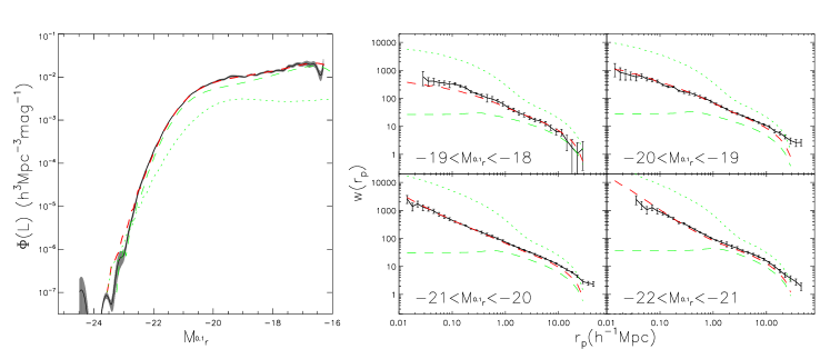
Our best fit model has the parameters: $M_{0}=3.41\times 10^{11}h^{-1}M_{\odot}$, $\alpha=0.221$, $\beta=1.67$, $k=8.13$ and $\sigma=0.440$ for the central galaxies and $M_{0}=2.58\times 10^{11}h^{-1}M_{\odot}$, $\alpha=0.345$, $\beta=3.83$, $k=7.71$ and $\sigma=0.742$ for the satellite galaxies (see Table 2). The resulting luminosity function and correlation functions are shown in Fig. 9. $\chi^{2}(\Phi)/N_{\Phi}$ is $3.348$ and the total $\chi^{2}$ is $6.115$. Also plotted are the results of central and satellite subsamples of our parametrized model, shown by green dashed and dotted lines. The drop in the correlation function on scales larger than $\sim 10h^{-1}$ Mpc is not caused by a poor fit; it is due to the truncation of our integration of the real space correlation function at $r=60h^{-1}$ Mpc^-1.

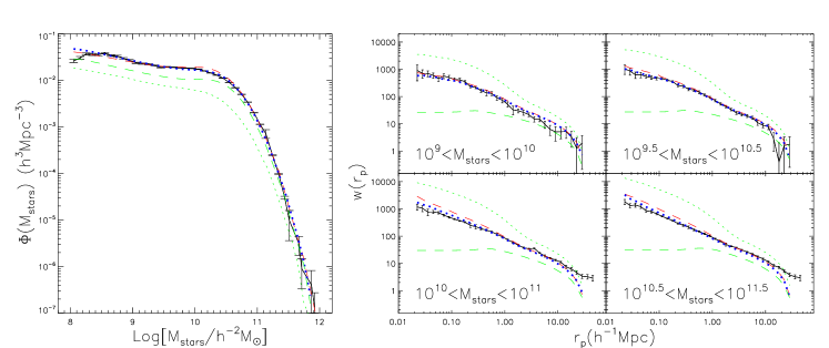
We now carry out the same analysis for stellar mass, rather than luminosity. We have constructed the stellar mass function directly from the SDSS DR2 data (Fig. 10; left panel) and use this, in conjunction with the measurements of $w(r_{p})$ as a function of stellar mass published by (Li et al., 2006), to constrain the $M_{stars}$-$M_{infall}$ relation. In the computation of stellar mass function, we have corrected for the volume effect by weighting each galaxy by a factor of $V_{survey}/V_{max}$, where $V_{survey}$ is the volume for the sample and $V_{max}$ is the maximum volume over which the galaxy could be observed within the sample redshift range ($0.01<z<0.3$) and within the range of $r-$band apparent magnitude ($14.5<r<17.77$). A Schechter function provides a good fit to our measurement at stellar mass $M_{stars}<10^{11.5}h^{-2}M_{\odot}$. We find best-fit parameters: $\Phi^{\ast}=(0.0204\pm 0.0001)h^{3}$Mpc^-3, $\alpha=-1.073\pm 0.003$ and $M^{\ast}_{stars}=(4.11\pm 0.02)\times 10^{10}h^{-2}M_{\odot}$. This corresponds to a stellar mass density of $(8.779\pm 0.067)\times 10^{8}hM_{\odot}$Mpc^-3.

We fit our models to $30$ points along the stellar mass function and $20$ points along the correlation function for five different stellar mass bins ranging from $10^{9}$ to $10^{12}M_{\odot}$. The parameters of the best-fit models are listed in Table 2. For the stellar mass function, the errors due to sample size are much smaller than the systematic errors in the stellar mass estimates themselves. We therefore assign the same error to all points at stellar masses less than $10^{11.5}h^{-2}M_{\odot}$ (the error is equal to the value at that mass). In our first attempt at fitting the data, we assumed that the $M_{stars}-M_{infall}$ would be the same for central and satellite galaxies, because the relations are very similar in the semi-analytic galaxy catalogues. The red dashed lines in Fig. 10 show the best fitting results. The model clearly over-predicts the clustering of the more massive galaxies on small scales. If we allow the relation between $M_{stars}$ and $M_{infall}$ to differ for central and satellite galaxies, we obtain the results shown by the blue dotted lines, which are considerably better.

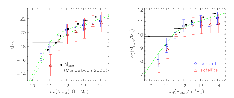
The best-fit $r$-band luminosity – $M_{infall}$ and $M_{stars}-M_{infall}$ relations derived from our models are illustrated in Fig. 11. Results are shown separately for central galaxies (blue) and satellite galaxies (red). In our models, satellite galaxies have lower luminosities and smaller stellar masses than central galaxies at a given value of $M_{infall}$. This effect is larger for luminosity than for stellar mass, particularly at low values of $M_{infall}$.

For comparison, we also plot the $L$-$M_{infall}$ and $M_{stars}-M_{infall}$ relations from the semi-analytic galaxy catalogue(Croton et al., 2006). We transform the $b_{j}$ band magnitude of semi-analytic catalogue to $r$ band in SDSS according to the luminosity functions of 2dFGRS(Madgwick et al., 2002) and SDSS(Blanton et al., 2003b), and make a shift of $0.9$ dex to do the comparison. Because Croton et al assumed a Salpeter initial mass function, the stellar mass-to-light ratios of the galaxies in their catalogue will be a factor of $\sim 2$ higher than in the SDSS data sample. This is because the stellar masses of Kauffmann et al. (2003) have been derived using a Kroupa (2001) IMF. As discussed by Kauffmann et al. (2003), the Salpeter IMF yields stellar masses for elliptical galaxies that exceed estimates of their dynamical masses(Cappellari et al., 2006). The Salpeter IMF is clearly unphysical and should be dropped. For the comparison shown in Fig. 11, we have simply scaled the stellar masses in the Croton et al catalogues by multiplying by a factor 0.5, which should give almost the same results as re-running the semi-analytic model with the Kroupa IMF. Compared with our results, the semi-analytic catalogue yields systematically higher luminosities and stellar masses at low values of $M_{infall}$, particularly for satellite galaxies. The agreement with the semi-analytic catalogue at $M_{infall}>10^{11.5}h^{-1}M_{\odot}$ is quite good.

Recently Mandelbaum et al. (2005) and Mandelbaum et al. (2006) have used galaxy-galaxy weak lensing measurements from SDSS data to explore the explore the connection between galaxies and dark matter. They compare the predicted lensing signal from a halo model constructed using a dissipationless simulation, and extract median/mean halo masses and satellite fractions for galaxies as a function of luminosity, stellar mass and morphology. We plot their estimates of the mean central halo mass as a function of $r$-band absolute magnitude and stellar mass as filled circles in Fig. 11. The results shown are the combined sample of early and late-type galaxies(Mandelbaum, private communication). These measurements should be compared with our blue points, which show the mean halo masses of present-day central galaxies. As can be seen, there is remarkably good agreement between the two methods, both for luminosity and for stellar mass.

6 Conclusions and Discussion

We have constructed a new statistical model of galaxy clustering for use in high resolution numerical simulations of structure formation. Unlike classic halo occupation distribution (HOD) models, galaxy positions and velocities are determined in a self-consistent way by following the full orbital and merging histories of all the haloes and subhaloes in the simulation. We believe that this methodology has advantages over the traditional approach. Most HOD models assume that the galaxy content of a halo of given mass is statistically independent of its larger scale environment. Recently (Gao et al., 2005) have shown that there exists an age dependence of halo clustering: haloes that are formed earlier are more clustered than haloes that are assembled more recently, indicating that this assumption may not be as safe as previously thought. Since the positions and the velocities of the galaxies in our model are determined directly from the simulation, we avoid these difficulties.

Our methodology also takes into account the contribution of “orphaned” galaxies, which have lost their halos due to tidal stripping. These galaxies contribute significantly to the clustering amplitude of low mass galaxies on scales less than $\sim 1h^{-1}$ Mpc. We have chosen to parametrize the observed properties of galaxies (in particular their luminosity and stellar mass) as a function of the quantity $M_{infall}$, the mass of the halo at the epoch when the galaxy was last the central object in its halo. Using the semi-analytic model results as a reference, we adopt a double power law form for this relation, and we show that this allows us to recover the mass/luminosity function and the correlation function in different ranges of mass and luminosity with high accuracy.

We then apply our model to measurements of these quantities using data from the Sloan Digital Sky Survey. We find that for a given value of $M_{infall}$, satellite galaxies are required to be less luminous and less massive than central galaxies. This effect is stronger at low values of $M_{infall}$. In the semi-analytic models, satellite galaxies fade in luminosity after they fall into a larger halo because they no longer accrete gas and their star formation rates then decline. The catalogues of Croton et al. (2006) do show differences between satellite and central galaxy luminosities at a fixed value of $M_{infall}$, but the effect is not quite as strong as the data demands, particularly for low mass halos. This may indicate that the efficiency with which baryons are converted into stars in low mass halos is higher at the present day than it was in the past. The fact that the standard $\Lambda$CDM model predicts more low mass galaxies than observed is very well-documented in the literature (Moore et al., 1999). Many authors have tried to invoke mechanisms for “suppressing” star formation in these systems (Kauffmann et al., 1993; Somerville, 2002) and most of these mechanisms operate more effectively at higher redshifts.

Finally, we compare our relations between galaxy luminosity, stellar mass and host halo mass with similar relations derived using galaxy-galaxy weak lensing measurements. The excellent agreement between these two completely independent methods is very encouraging.

References

- Arnaboldi (2004) Arnaboldi M., 2004, in Duc P.-A., Braine J., Brinks E., eds, IAU Symposium Intracluster Stellar Population. pp 54–+
- Benson et al. (2000) Benson A. J., Cole S., Frenk C. S., Baugh C. M., Lacey C. G., 2000, MNRAS, 311, 793
- Berlind & Weinberg (2002) Berlind A. A., Weinberg D. H., 2002, ApJ, 575, 587
- Berlind et al. (2003) Berlind A. A., Weinberg D. H., Benson A. J., Baugh C. M., Cole S., Davé R., Frenk C. S., Jenkins A., Katz N., Lacey C. G., 2003, ApJ, 593, 1
- Blanton et al. (2003a) Blanton M. R., Brinkmann J., Csabai I., Doi M., Eisenstein D., Fukugita M., Gunn J. E., Hogg D. W., Schlegel D. J., 2003a, AJ, 125, 2348
- Blanton et al. (2003b) Blanton M. R., Hogg D. W., Bahcall N. A., Brinkmann J., Britton M., Connolly A. J., Csabai I., Fukugita M., et al., 2003b, ApJ, 592, 819
- Cappellari et al. (2006) Cappellari M., Bacon R., Bureau M., Damen M. C., Davies R. L., de Zeeuw P. T., Emsellem E., Falcón-Barroso J., Krajnović D., Kuntschner H., McDermid R. M., Peletier R. F., Sarzi M., van den Bosch R. C. E., van de Ven G., 2006, MNRAS, 366, 1126
- Colless et al. (2001) Colless M., Dalton G., Maddox S., Sutherland W., Norberg P., Cole S., Bland-Hawthorn J., Bridges T., et al., 2001, MNRAS, 328, 1039
- Conroy et al. (2005) Conroy C., Wechsler R. H., Kravtsov A. V., 2005, astro-ph/0512234
- Croton et al. (2006) Croton D. J., Springel V., White S. D. M., De Lucia G., Frenk C. S., Gao L., Jenkins A., Kauffmann G., Navarro J. F., Yoshida N., 2006, MNRAS, 365, 11
- De Lucia et al. (2004) De Lucia G., Kauffmann G., Springel V., White S. D. M., Lanzoni B., Stoehr F., Tormen G., Yoshida N., 2004, MNRAS, 348, 333
- Feldmeier et al. (2004) Feldmeier J. J., Mihos J. C., Morrison H. L., Harding P., Kaib N., Dubinski J., 2004, ApJ, 609, 617
- Gao et al. (2004) Gao L., De Lucia G., White S. D. M., Jenkins A., 2004, MNRAS, 352, L1
- Gao et al. (2005) Gao L., Springel V., White S. D. M., 2005, MNRAS, 363, L66
- Hawkins et al. (2003) Hawkins E., Maddox S., Cole S., Lahav O., Madgwick D. S., Norberg P., Peacock J. A., Baldry I. K., et al., 2003, MNRAS, 346, 78
- Katz et al. (1996) Katz N., Weinberg D. H., Hernquist L., 1996, ApJS, 105, 19
- Kauffmann et al. (1999) Kauffmann G., Colberg J. M., Diaferio A., White S. D. M., 1999, MNRAS, 303, 188
- Kauffmann et al. (2003) Kauffmann G., Heckman T. M., White S. D. M., Charlot S., Tremonti C., Brinchmann J., Bruzual G., Peng E. W., et al., 2003, MNRAS, 341, 33
- Kauffmann et al. (1997) Kauffmann G., Nusser A., Steinmetz M., 1997, MNRAS, 286, 795
- Kauffmann et al. (1993) Kauffmann G., White S. D. M., Guiderdoni B., 1993, MNRAS, 264, 201
- Kroupa (2001) Kroupa P., 2001, MNRAS, 322, 231
- Li et al. (2006) Li C., Kauffmann G., Jing Y. P., White S. D. M., Börner G., Cheng F. Z., 2006, MNRAS, 368, 21
- Madgwick et al. (2002) Madgwick D. S., Lahav O., Baldry I. K., Baugh C. M., Bland-Hawthorn J., Bridges T., Cannon R., Cole S., et al., 2002, MNRAS, 333, 133
- Mandelbaum et al. (2006) Mandelbaum R., Seljak U., Kauffmann G., Hirata C. M., Brinkmann J., 2006, MNRAS, 368, 715
- Mandelbaum et al. (2005) Mandelbaum R., Tasitsiomi A., Seljak U., Kravtsov A. V., Wechsler R. H., 2005, MNRAS, 362, 1451
- Moore et al. (1999) Moore B., Ghigna S., Governato F., Lake G., Quinn T., Stadel J., Tozzi P., 1999, ApJ, 524, L19
- Norberg et al. (2002a) Norberg P., Baugh C. M., Hawkins E., Maddox S., Madgwick D., Lahav O., Cole S., Frenk C. S., et al., 2002a, MNRAS, 332, 827
- Norberg et al. (2002b) Norberg P., Cole S., Baugh C. M., Frenk C. S., Baldry I., Bland-Hawthorn J., Bridges T., Cannon R., et al., 2002b, MNRAS, 336, 907
- Peacock & Smith (2000) Peacock J. A., Smith R. E., 2000, MNRAS, 318, 1144
- Pearce et al. (2001) Pearce F. R., Jenkins A., Frenk C. S., White S. D. M., Thomas P. A., Couchman H. M. P., Peacock J. A., Efstathiou G., 2001, MNRAS, 326, 649
- Seljak (2000) Seljak U., 2000, MNRAS, 318, 203
- Somerville (2002) Somerville R. S., 2002, ApJ, 572, L23
- Spergel et al. (2003) Spergel D. N., Verde L., Peiris H. V., Komatsu E., Nolta M. R., Bennett C. L., Halpern M., Hinshaw G., et al., 2003, ApJS, 148, 175
- Springel et al. (2005) Springel V., White S. D. M., Jenkins A., Frenk C. S., Yoshida N., Gao L., Navarro J., Thacker R., et al., 2005, Nature, 435, 629
- Springel et al. (2001) Springel V., White S. D. M., Tormen G., Kauffmann G., 2001, MNRAS, 328, 726
- Vale & Ostriker (2004) Vale A., Ostriker J. P., 2004, MNRAS, 353, 189
- Vale & Ostriker (2005) Vale A., Ostriker J. P., 2005, astro-ph/0511816
- van den Bosch et al. (2003) van den Bosch F. C., Yang X., Mo H. J., 2003, MNRAS, 340, 771
- Wang et al. (2004) Wang Y., Yang X., Mo H. J., van den Bosch F. C., Chu Y., 2004, MNRAS, 353, 287
- White et al. (2001) White M., Hernquist L., Springel V., 2001, ApJ, 550, L129
- Yang et al. (2005) Yang X., Mo H. J., Jing Y. P., van den Bosch F. C., 2005, MNRAS, 358, 217
- Yang et al. (2003) Yang X., Mo H. J., van den Bosch F. C., 2003, MNRAS, 339, 1057
- York et al. (2000) York D. G., Adelman J., Anderson J. E., Anderson S. F., Annis J., Bahcall N. A., Bakken J. A., Barkhouser R. a., 2000, AJ, 120, 1579
- Yoshikawa et al. (2001) Yoshikawa K., Taruya A., Jing Y. P., Suto Y., 2001, ApJ, 558, 520
- Zehavi et al. (2004) Zehavi I., Weinberg D. H., Zheng Z., Berlind A. A., Frieman J. A., Scoccimarro R., Sheth R. K., Blanton M. R., et al., 2004, ApJ, 608, 16
- Zehavi et al. (2005) Zehavi I., Zheng Z., Weinberg D. H., Frieman J. A., Berlind A. A., Blanton M. R., Scoccimarro R., Sheth R. K., et al., 2005, ApJ, 630, 1
- Zibetti et al. (2005) Zibetti S., White S. D. M., Schneider D. P., Brinkmann J., 2005, MNRAS, 358, 949