Inflation models after WMAP year three

Abstract

The survey of models in astro-ph/0510441 is updated. For the first time, a large fraction of the models is ruled out at more than $3\sigma$.

I Introduction

In a recent paper al we discussed a range of models for the origin of the curvature perturbation and the tensor perturbation, including constraints on the spectral index $n$ coming from WMAP year one data. In this note we update the discussion to include WMAP year three data wmap3 . The models assume that the curvature perturbation is generated from the vacuum fluctuation of the inflaton field, so that it is directly related to the inflationary potential. Some of them work with the type of field theory that is usually invoked when considering extensions of the Standard Model, while others work within a framework derived more or less directly from string theory.

The prediction for $n$ typically depends on $N$, the number of $e$-folds of slow-roll inflation occurring after the observable Universe leaves the horizon. With a high inflation scale, and radiation and/or matter domination between the end of inflation and nucleosynthesis,

$$N=54\pm 7.$$ (1)

More generally the range has to be

$$14<N<75,$$ (2)

the lower bound coming from the requirement to form early objects weighing a million solar masses, and the upper bound from imposing $P/\rho<1$ on the pressure and energy density andrewn .

Following al , we call a model small-field if the change $\Delta\phi_{N}$ of the inflaton field during the $N$ $e$-folds is $\lesssim M_{\rm P}$, and large-field if it is $\gg M_{\rm P}$.

II Small-field models

II.1 A class of allowed models

Assuming that the tensor fraction $r$ is negligible and that the spectral tilt $n-1$ is practically constant while cosmological scales leave the horizon, the WMAP constraint is

$$n=0.948^{+0.015}_{-0.018}.$$ (3)

This is actually the constraint obtained by combining WMAP data with the SDSS galaxy survey, but it hardly changes if some other data sets are used, including WMAP alone.

Essentially the same constraint was obtained using WMAP year one data, in conjunction with the 2dF galaxy survey alone 2dfwmap or with 2dF and other data sets wbs2 , but a higher result compatible with $n=1$ was obtained using WMAP year one data alone or WMAP with sdsswmap SDSS. The crucial point now is that even in the last two cases the scale-invariant value $n=1$ is excluded at around the $3\sigma$ level.

For small-field models with a concave-downward potential, $\epsilon\lesssim 0.0002$ hilltop . Then the prediction ll92 $n=1+2\eta-6\epsilon$ becomes just $n=1+2\eta$. For a wide class of concave-downward models this becomes treview

$$n=1-\frac{p-1}{p-2}\frac{2}{N},$$ (4)

with $p\gtrsim 3$ or $p\leq 0$. (Here $N$ is actually $N(k)\equiv N-\ln(H_{0}/k)$, but the variation presumably is negligible over the range $\Delta N\sim 10$ over which the observational constraint applies.) For these models, the observed normalization of the spectrum requires a high inflation scale, so that Eq. (1) will be appropriate for a standard post-inflationary cosmology, but still the tensor fraction is negligible.

The case $p\leq 0$ is realised in some hybrid inflation models in which the potential necessarily steepens significantly towards the end of inflation. The case $p<0$ corresponds to a potential

$$V\simeq V_{0}\left[1-\left(\frac{\phi}{\mu}\right)^{p}\right],$$ (5)

with $V_{0}$ dominating so as to permit inflation. This can come from mutated hybrid inflation mutated ; inverted , with integer values of $p$ favoured but not mandatory. With integral $p$ it can also come from $N=2$ supergravity juann2 or D-brane cosmology dbraneinf . The limit $p\to 0$ corresponds to a logarithmic potential achieved in the simplest and perhaps unrealistic version of $F$-term cllsw ; fterm ; ewanexp or $D$-term ewanexp ; dterm hybrid inflation. The limit $p\to-\infty$ corresponds to an exponential potential, which may be generated by a kinetic term passing through zero ewanexp or by by appropriate non-Einstein gravity (non-hybrid) inflation treview (see also cq ).

The case $p\gtrsim 3$ also corresponds to Eq. (5). This case is attractive because it gives the potential a maximum, at which eternal inflation can take place providing the initial condition for the subsequent slow roll eternal1 ; eternal2 ; hilltop . As Eq. (5) is only supposed to be an approximation lasting for a sufficient number of $e$-folds, $p$ need not be an integer, but it has to be well above $2$ for the prediction (4) to hold. It could correspond to non-hybrid inflation with $\Delta\phi\ll M_{\rm P}$ (New Inflation new ; sv ) or else with $\Delta\phi\sim M_{\rm P}$ (Modular Inflation which has a long history andrei83 ; modular1 ; graham and is currently under intense investigation in the context of string theory modular2 ; more ; west ). It could also correspond to mutated hybrid inflation inverted , or else hilltop to one of the $p\leq 0$ models, modified by the addition of a non-renormalizable term.

An attractive proposal which can give Eq. (4) is to make the inflaton a pseudo-Nambu-Goldstone boson so that the flatness of its potential is protected by a symmetry. Realizations of this proposal include a two-component model giving $p=3$ cs and a hybrid model giving $p=0$ pseudonat . (A different proposal for ensuring the flatness is described in glm based on earlier work cllsw ; ewanexp , but it has not been carried through to the point where a definite form for the potential is proposed.)

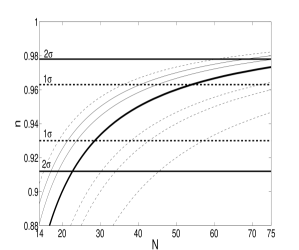
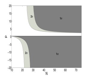
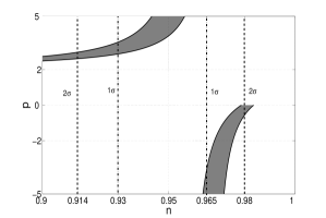
In Figure 1, the prediction (4) is shown against $N$ for a few values of $p$. Very low values of $N$ are forbidden, as is seen clearly in Figure 2. With $N$ in the reasonable range (1), the prediction $n(p)$ is shown in Figure 3, where we see that all values of $p$ are just about allowed at the $2\sigma$ level.

Figure 1: The prediction (4) for different $p$. The bold full line is the limit $|p|\to\infty$. Above it from top down are the lines $p=0$, $-2$ and $-4$, and below it from bottom up are the lines $p=3$, $4$ and $5$. The observational bounds from wmap3 are indicated.

Figure 2: The regions excluded by the observational bounds from wmap3 , for the parameter $p$ in the prediction (4).

Figure 3: The prediction (4) for $N=54\pm 7$.

Figure 4: The curved lines are the Natural Inflation predictions for $N=20$, $N=54$ and $N=75$, and the horizontal lines are the corresponding multi-component Chaotic Inflation predictions. The junction of each pair of lines corresponds to single-component Chaotic Inflation. The regions allowed by observation with various assumptions are taken from wmap3 .

These cases give a spectral index more or less in agreement with the observed one because their prediction is $n-1\simeq-1/N$. The case of Eq. (5) with $p=2$ is quite different. The tilt is now $n-1=-2\mu^{2}M_{\rm P}^{2}/V$, which might have had any value in the range $-1\ll n-1<0$. It depends on the parameters of the potential, not just on its functional form as in the previous case.

Now that observation requires such a small tilt, the case $p=2$ actually looks rather problematic because it requires a rather abrupt steepening of the potential after cosmological scales leave the horizon. This is difficult to achieve in a non-hybrid model; for instance the Little-Higgs proposal of pseudonat seems not to give a sufficiently abrupt end. It can be achieved in an inverted hybrid model inverted by choice of parameters, but this typically involves fine-tuning steveinvert , and the negative coupling of the inflaton to the waterfall field is non-standard and difficult to achieve in the context of supersymmetry.

II.2 Models ruled out

If the observation of negative tilt holds up it will represent a very significant development. Speaking generally, it avoids the criticism that $n=1$ might have had some simple explanation, overlooked so far, which has nothing to do with field theory or inflation. Within the context of slow-roll inflation, $n=1$ excludes several possibilities for the inflationary potential in a small-field model.

Concave-upward potentials

A concave-upward potential give positive tilt if $2\eta>6\epsilon$. That is generally the case for small-field models. In particular it is true for small-field models with

$$V=V_{0}\left[1+\left(\frac{\phi}{\mu}\right)^{p}\right].$$ (6)

Indeed, $V_{0}$ must dominate to achieve small-field inflation, but then $\epsilon\sim(\phi/M_{\rm P})^{2}\eta^{2}\ll\eta$. An attractive realization of this potential is the original hybrid model with $p=2$. An integer $p\geq 3$ also corresponds to tree-level hybrid inflation, andreihybrid ; hybrid2 ; inverted while the case $p\leq-1$ corresponds to dynamical supersymmetry breaking dsb . These are less attractive because small-field inflation occurs only over a limited range of $\phi$ and it is not clear how the field is supposed to arrive within this range treview .

Very flat potentials

If the potential is very flat, $\epsilon$ and $\eta$ will be negligible and so will the tilt $n-1$. This happens in some models which seek to explain the inflationary scale $V$ by identifying it with the scale of supersymmetry breaking in the vacuum supernatural ; steve ; dr . The models make the very potential flat in order to reproduce the observed spectrum ${\cal P}_{\zeta}=(5\times 10^{-5})^{2}$ with the formula ${\cal P}_{\zeta}\simeq(V/\epsilon M_{\rm P}^{4})$ and the low scale $V^{1/4}\lesssim 10^{10}\,\mbox{GeV}$ assumed for supersymmetry breaking. Such models are accordingly ruled out by the observed tilt.

Running Mass inflation

The idea of running mass inflation is to use a loop correction, to flatten a tree-level potential, which would otherwise be too steep for inflation. The model of ewanrunning ; cl uses a tree-level quadratic potential (Eq. (6) with $p=2$) modified by a one-loop correction. It is assumed that the tree-level potential has $\eta\sim 1$, which is the generic supergravity value and marginally spoils inflation. This model gives significant positive running of the spectral index $dn(k)/dk>0$, which was allowed by the WMAP year one data ourrunning if $n$ passed through zero around the the middle of the cosmological range of scales. The model presumably is ruled out by the WMAP three year data, which allows $n(k)$ to pass through 1 only in the negative direction. The alternative model of ks makes inflaton is a two-component modulus. It typically gives either negligible tilt or tilt with rather strong running, but further investigation is needed to see whether it is ruled out.

Generic modular inflation and supergravity

A string theory modulus is expected generically to have a potential of the form $V=V_{0}f(\phi/M_{\rm P})$, with $f(x)$ and its low derivatives of order 1 at a generic point in the range $\phi\lesssim M_{\rm P}$. Near a maximum this gives $\eta\sim-1$ which only marginally allows inflation and gives $n-1\sim-1$. A similar result, $|\eta|\gtrsim 1$, is expected in a generic supergravity theory for any field. One of the most significant consequences of the bound $|n-1|\lesssim 0.1$, which observation has provided in recent years, is that $|\eta|$ has to be reduced below its generic value by more than a factor $10$. The new result for $n-1$ confirms that, but it also assures us that we will not have to go much further. Inflation based on a modulus and/or supergravity requires fine-tuning of $\eta$ at the few percent level, but not worse. More fine-tuning is typically needed though, to stabilize fields other than $\phi$.

III Large-field models

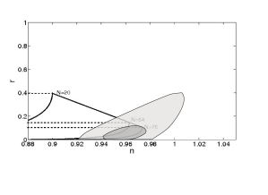
Large-field models allow an observable tensor fraction $r$. The single-component models are chaotic inflation chaotic , the multi-component version of that starob85 ; Nflation , and Natural Inflation natural . The situation for these models is illustrated in Figure 4. (It shows the WMAP/SDSS constraint, but but it hardly changes if WMAP is combined with other data sets.) There is no dramatic change from the situation with earlier constraints derived from WMAP year-one.

The generic prediction for a chaotic inflation potential $V\propto\phi^{\alpha}$ is

$$r = \frac{4\alpha}{N}$$ (7)

$$n-1 = 2\eta-6\epsilon=-\frac{2+\alpha}{2N}.$$ (8)

As pointed out already wmap3 , the year-three WMAP data rule out rather firmly $\alpha\geq 4$. Interestingly enough, the allowed case $\alpha=2$ is also the best-motivated one in the context of received ideas about field theory extranat ; pseudonat ; Kim:2004rp , because it is reproduced by a Natural Inflation potential with a large period.

IV Summary and outlook

Over the last twenty-five years many field-theory models of slow-roll inflation have been proposed. We have seen that the WMAP year three results for $n$ and $r$ rule out a large fraction of these models. The remainder seem to be in three broad classes; large field models, small-field models giving the prediction (1) with $p\leq 0$, and small-field models giving the same prediction with $p\gtrsim 3$. Within a few years, the PLANCK result for $n$ and the Clover result for $r$ will almost certainly rule out at least two of these classes, and provide some discrimination within the remaining class.