An Upper Limit on the Albedo of HD 209458b:
Direct Imaging Photometry with the MOST Satellite

Abstract

We present space-based photometry of the transiting exoplanetary system HD 209458 obtained with the MOST (Microvariablity and Oscillations of STars) satellite, spanning 14 days and covering 4 transits and 4 secondary eclipses. The HD 209458 photometry was obtained in MOST’s lower-precision Direct Imaging mode, which is used for targets in the brightness range $6.5\geq V\geq 13$. We describe the photometric reduction techniques for this mode of observing, in particular the corrections for stray Earthshine. We do not detect the secondary eclipse in the MOST data, to a limit in depth of 0.053 mmag ($1\sigma$). We set a 1$\sigma$ upper limit on the planet-star flux ratio of $4.88\times 10^{-5}$ corresponding to a geometric albedo upper limit in the MOST bandpass (400 to 700 nm) of 0.25. The corresponding numbers at the $3\sigma$ level are $1.34\times 10^{-4}$ and 0.68 respectively. HD 209458b is half as bright as Jupiter in the MOST bandpass. This low geometric albedo value is an important constraint for theoretical models of the HD209458b atmosphere, in particular ruling out the presence of reflective clouds. A second MOST campaign on HD 209458 is expected to be sensitive to an exoplanet albedo as low as 0.13 (1$\sigma$), if the star does not become more intrinsically variable in the meantime.

1 Introduction

Since the discovery of the giant planet orbiting 51 Pegasi (Mayor& Queloz, 1995) a decade ago, and the subsequent detection of about 160 exoplanetary systems around solar-type stars (Schneider, 2005), the task of acquiring information about the atmospheres of giant close-in planets has been particularly challenging. Observations of the transits of the exoplanet HD 209458b have revealed the presence of sodium in its atmosphere (Charbonneau et al., 2002) and a hydrogen cloud around it (Vidal-Madjar et al., 2003). The Spitzer infrared space observatory has detected the eclipse of HD 209458b in its thermal emission at 24-$\mu$ (Deming et al., 2005a), yielding a brightness temperature at that wavelength of $1130\pm 150$ K.

We report here an attempt to detect the eclipse of HD 209458b (orbital period $\sim$ 3.5 d) in reflected light at optical wavelengths, with photometry from the MOST (Microvariablity and Oscillations of STars) satellite (Walker, Matthews et al., 2003; Matthews et al., 2004). The reflected light signal from an exoplanet is sensitive to the composition of its atmosphere, as well as the nature and filling factor of cloud particles suspended in that atmosphere (Seager et al., 2000; Green et al., 2003; Burrows et al., 2005). The proportion of scattered to absorbed radiation is critical to the planet’s energy balance and hence an albedo measurement is key to understanding its atmosphere.

The MOST satellite houses a 15-cm optical telescope feeding a CCD photometer through a single broadband filter (350 - 750 nm), which is capable of sampling target stars up to 10 times per minute. From the vantage point of its 820-km-high circular Sun-synchronous polar orbit with a period of 101.413 minutes, MOST can monitor stars nearly continuously for up to 8 weeks in a Continuous Viewing Zone (CVZ) with a declination range of $+36^{\circ}\geq\delta\geq-18^{\circ}$. The satellite was designed to achieve photometric precision of a few parts per million (ppm $\sim\mu$mag) at frequencies ($>$ 1 mHz) in the Fourier domain. The necessary photometric stability is achieved by projecting an extended image of the instrument pupil illuminated by the Primary Science Target via one of an array of Fabry microlenses above the MOST Science CCD (a 1K $\times$ 1K E2V 47-20 detector). For exposure times up to 1 minute long, and observing runs of at least 1 month, this Fabry Imaging mode can reach the desired precision of about 1 ppm at frequencies greater than 1 mHz for stars brighter than V $\sim$ 6.5.

Fainter stars can be monitored (simultaneously, or independently of the Fabry Imaging mode) in an open area of the Science CCD not covered by the $6\times 6$ Fabry microlens array and its chromium field stop mask. In the Direct Imaging field, defocused star images are projected, with a Full-Width Half-Maximum (FWHM) of about 2.5 pixels. (The focal plane scale of MOST is about 3 arcsec/pixel.) The photometric precision possible in the Direct Imaging Mode is not as good as for the Fabry photometry as Direct Imaging targets are fainter and more sensitive to CCD calibrations. However, the unprecedented duty cycle of the MOST observations and the thermal/mechanical stability of the instrument yield impressive results. The point-to-point precision of the photometry reported here is about 3 millimag for a 1.5s exposure during low stray light conditions, with sampling rates as high as 10 exposures per minute and a duty cycle of 85% in 14 days of observation, where a duty cycle of 100% represents no loss of data acquisition.

Photometry of this quality and coverage represents a unique opportunity to explore the HD 209458 transiting system. The star is not too bright for the MOST Direct Imaging mode ($V=7.65$) and it is well placed in the MOST CVZ, observable for up to about a month and a half. MOST data have many applications to this system: (1) accurate transit timing to refine the near-zero orbital eccentricity and check for effects of orbital precession; (2) studies of the shapes of transit ingress and egress to search for large moons around HD 209458b; (3) searching for transits of other smaller planets in the systems with different orbital periods, as predicted by some models to explain the dynamical stability of HD 209458b (e.g., Ida & Lin (2004)); (4) revealing subtle intrinsic variability in the star HD 209458a and possible interactions with the close-in planet; and (5) detection of the eclipse of HD 209458b in optical light to directly measure the geometric albedo of the planet.

In this paper, we report on MOST observations and analysis for eclipse detection in this system. In the next two sections, we describe the data and the MOST Direct Imaging reduction scheme, as a reference for MOST Direct Imaging results published here and elsewhere. We then present the reduced photometry of HD 209458, the eclipse analysis, and the upper limit on the depth of the eclipse. We translate this into an upper limit on the optical albedo of the exoplanet, and discuss its implications in atmosphere and cloud models. Finally, we predict the impact of future planned MOST observations of HD 209458 and the potential for other known transiting exoplanet systems.

2 MOST Direct Imaging Photometry

MOST is a microsatellite (mass = 54 kg; peak solar power = 39 W) with limited onboard processing capability, memory, and downlink. Hence it is not possible to transfer the entire set of $1024\times 1024$ pixels of the Science CCD to Earth at a rapid sampling rate and with an ADC (Analogue-to-Digital Conversion) of 14 bits (necessary to preserve variability information at the ppm level). Small segments of the CCD (”subrasters”) are stored, which contain key portions of the target field. This usually includes the Primary Science Target Fabry Image, 7 adjacent Sky Background Fabry Images, and subrasters for dark and bias readings.

2.1 Data Format

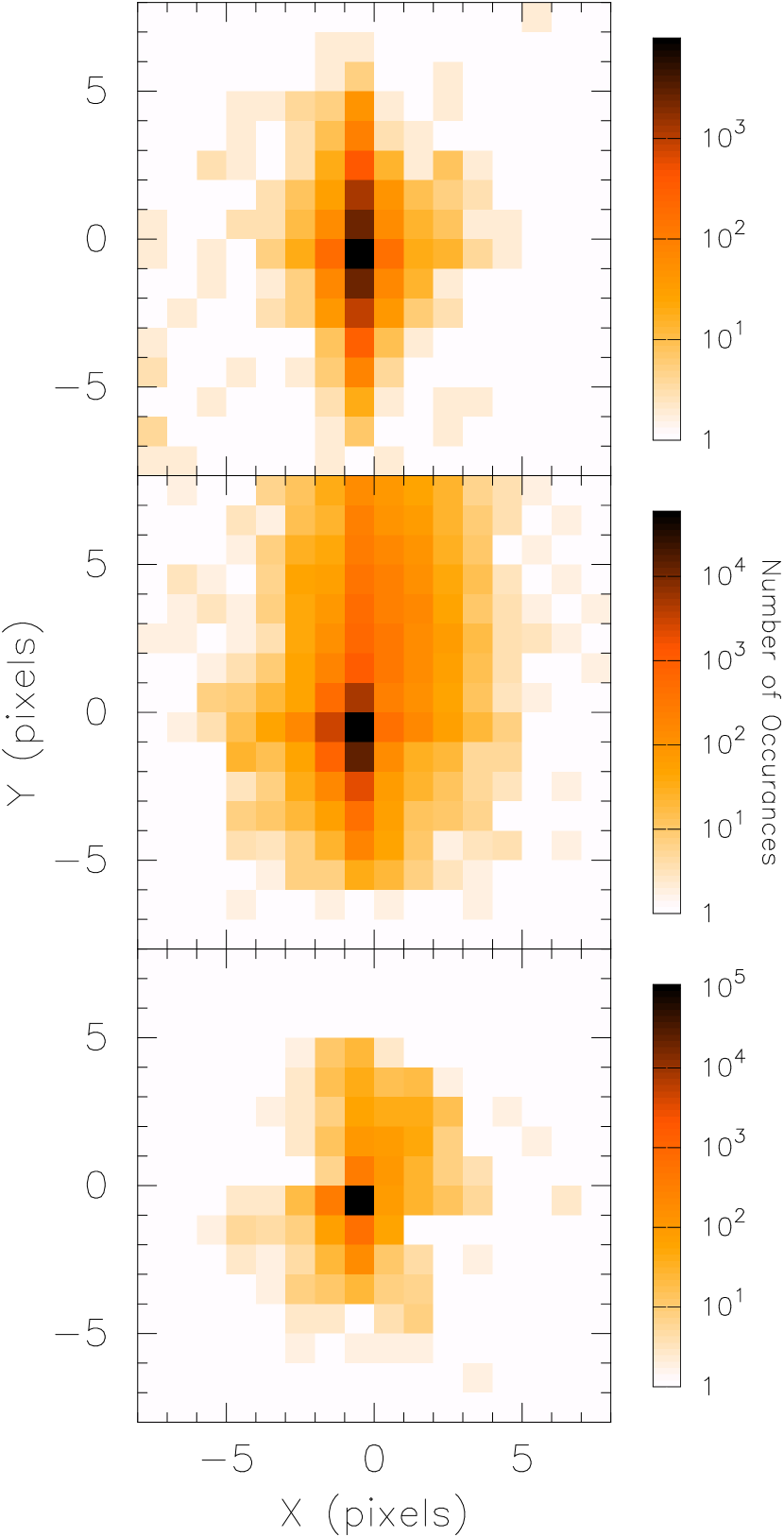
Figure 2: The pointing performance for three different targets. HD 263551 is shown in the top panel, HD 61199 in the middle panel and HD 209458 in the bottom panel. The top panel represents the typical point performance in early satellite operations. There is a substantial drift in the Y-direction. In the middle panel, the Y-axis drift has been largely eliminated. The bottom panel shows the current and much improved pointing performance.

There is also the option to sample several nearby Secondary Science Targets in the Direct Imaging field (less than about $0.5^{\circ}$ away), by placing subrasters of typical dimensions $20\times 20$ pixels over those stars. These targets are automatically monitored with the same sampling as the Primary Fabry Imaging target. The Fabry Image illuminates about 1500 pixels, while each Direct Image illuminates a PSF out to a radius of several pixels. When simultaneously observing Fabry and Direct Imaging targets to avoid saturation, the Direct Imaging Targets must be at least 5.5 magnitudes fainter than the Fabry Target. For example, for MOST’s first Primary Science Target, Procyon, the $V=8$ star HD 61199 was chosen for the Direct Imaging field and was discovered to be a multiperiodic $\delta$ Scuti pulsator (see Fig. 2c in Matthews et al. (2004)) with a peak amplitude of about 1 millimag .

It is also possible to select a star as bright as $V=6.5$ as the principal science target in the Direct Imaging field, without a brighter Fabry target. Then the exposure time and sampling rate can be optimized for the Direct Imaging target. This was the case for HD 209458 (V=7.7).

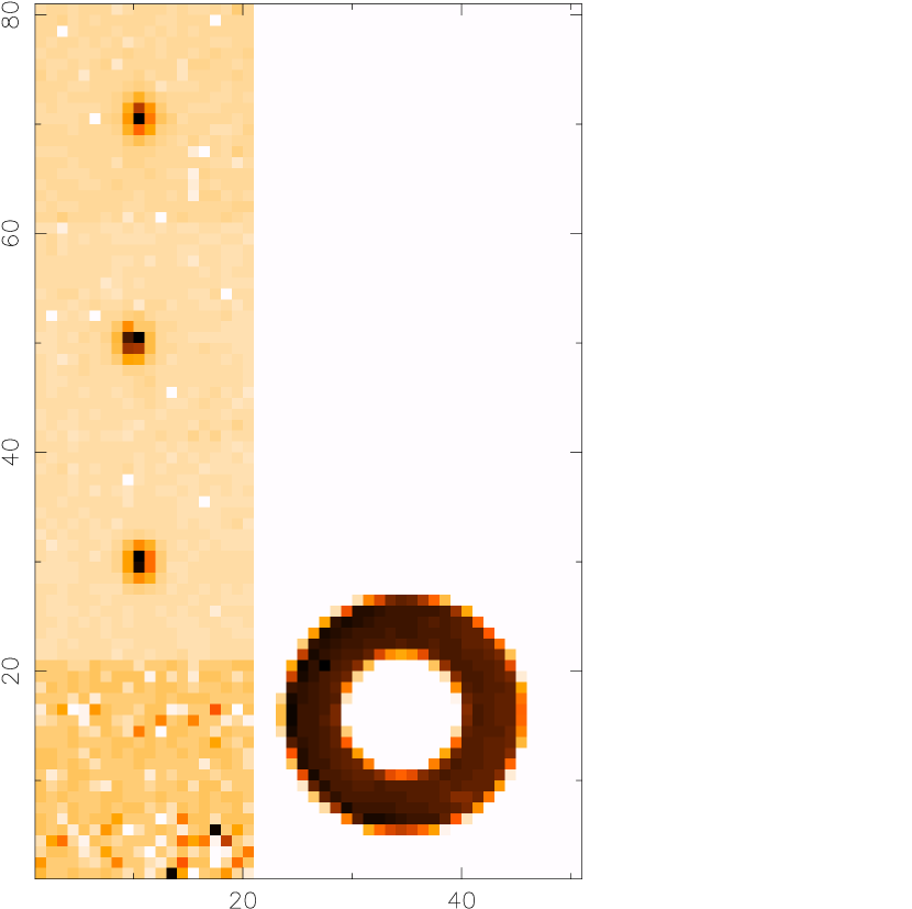
Figure 1: The FITS file layout is shown. There are 5 subrasters visible in this example, 3 containing stellar direct images, the Fabry projection and region shielded from light. The axis units are in pixels. The Fabry image has been binned 2x2.

When the binary data stream is transfered from the satellite it is converted to a FITS format image. The layout is shown in Figure 1. The locations of each subraster in the MOST Science CCD (in x-y pixel coordinates) are specified in the FITS file header. Typically, the FITS file contains resolved subrasters for the Fabry image, 2-4 Direct images and 1 dark. The header also contains the pixel sums for various bias and dark regions, as well as satellite and instrument telemetry (e.g., spacecraft attitude control data; CCD focal plane temperatures) to allow additional photometric calibrations on the ground. The data format is unique to MOST, which necessitated the development of custom software to handle and process MOST data. Examples of MOST raw data and a document describing the FITS file and header format in detail are available in the MOST Public Data Archive at the MOST Mission website: www.astro.ubc.ca/MOST.

2.2 Photometric Reduction

In general, the approach to reducing MOST Direct Imaging photometry is similar to groundbased CCD photometry, applying traditional aperture and PSF (Point-Spread Function) approaches to the subrasters. However, there are several aspects and challenges specific to MOST data. For example, the MOST instrument has no on-board calibration lamp for correction of pixel-to-pixel sensitivity variations (”flatfielding”). In its orbit, MOST passes through a region of enhanced cosmic ray flux known as the South Atlantic Anomaly (SAA). There are also phases of increased stray light from scattered Earthshine which repeat regularly during each satellite orbit ($P=101$ min).

2.2.1 Dark Correction

To lower cost and increase reliability, the MOST instrument has no moving parts, so there is no mechanical shutter which can cut off light to the entire CCD for dark measurements; exposures are ended by rapid charge transfer into a frame buffer on the CCD. Dark measurements are obtained from portions of the CCD shielded from light by a chromium mask above the focal plane.

One-dimensional dark current correction is done by using averages from these dark subrasters; the averages are computed on the satellite and the full raster information is not available on the ground (to meet downlink limitations while maximizing the amount of stellar data available). The values for each dark region are weighted in the average by the number of pixels in each subraster. There are usually 4 dark measurements available. If any of these individual readings deviates strongly (by more than 3$\sigma$) from the mean (likely due to a particularly energetic cosmic ray hit), then that value is discarded.

2.2.2 Flatfield Corrections

The MOST instrument was designed to obtain fixed extended pupil images of a single bright target star through a Fabry microlens. In this way, the Fabry Imaging measurements are insensitive to pointing wander of the satellite. The Direct Images, however, do reflect the pointing errors. In data from the satellite commissioning and its early scientific operations, pointing errors of up to about 10 arcsec led to wander of the Direct Images of up to 3 pixels on the CCD. This made precision photometry vulnerable to uncalibrated sensitivity variations among adjacent pixels. The pointing performance of the satellite has been improved dramatically since its early operation, now consistently giving positional errors of about $\pm 1$ arcsec $\sim$ 0.3 pixel $rms$ (see §2.2.3).

Despite the lack of an on-board calibration lamp, it is possible to recover some flatfielding information for each subraster by exploiting intervals of high stray light during certain orbital phases. Frames containing no detectable stars are chosen from the data set. Such frames can be obtained when the satellite is commanded to point to an “empty” field (with only stars much fainter than V = 13), or occasionally, when the satellite loses fine pointing and the stars wander outside their respective subrasters. During two weeks of observing, over which 50,000 - 100,000 individual exposures are typically obtained, about 2000 - 4000 flatfielding frames are usually available from when the satellite loses fine pointing.

The stray light can produce a strong spatial gradient across the CCD, so a 2-dimensional polynomial is fitted to all the available flatfielding pixels and removed. For each subraster, the mean pixel value is measured and compared to each individual pixel value; a linear fit to the correlation is made. The slope of this relationship is the relative gain and the zero point is the dark current. The relative pixel gains are found to vary by less than 2% across any individual subraster, with the standard deviation for any individual pixel less than 0.5%.

2.2.3 Star Detection and Centroiding

We employ two methods for star identification. The first method involves deconvolving the individual subrasters with a model Point-Spread Function (PSF). The model PSF is created by registering subrasters containing stars and mapping the pixel values onto an oversampled grid to create a model profile with twice the resolution of a real image. After deconvolution, the strongest source is chosen as the target star for photometry. The second method starts by prompting the user to identify by eye stars on each subraster via a graphical interface, which is particularly useful for fields containing several stars.

Once the stars have been identified, centroids are computed by an intensity-weighted average on a 5x5 grid around each object of interest. On the first frame, the centroids for all the stars are saved as a master grid used to check the positioning for all subsequent frames. After the first frame the strongest source is always selected using the deconvolution technique and its position is calculated with intensity-weighted means. This is done for each subraster and the offsets are compared to the master grid of centroids. If the position of a star varies by more than 2 pixels, then that centroid is corrected by using the average offset from the remaining objects. This correction is particularly important when cosmic rays interact with the detector and can mimic a stellar PSF, leading to the occasional spurious star identification.

The pointing performance of MOST has been dramatically improved since its original on-orbit commissioning, thanks to upgraded software and a better understanding of the mechanical performance of the reaction wheels in its attitude control system. In Figure 2, the distribution of pointing centroids for three fields observed from December 2003 to August 2004 are shown. The first is for the star HD 263551 in the field of $\xi$ Geminorum (observed during 20 - 28 December 2003); the second, for HD 61199 in the field of Primary Target Procyon (8 January - 9 February 2004); and the third, for HD 209458 itself (14 - 30 August 2004). The standard deviation for each target in x and y pixel directions are (0.985,1.945), (0.947,1.837), and (0.309,0.403), respectively. The substantial improvement in tracking stability has resulted in improved photometry precision as flat fielding errors have become less relevant.

2.2.4 Stray Light and Background Determination

In order to remove the strong background gradients associated with stray light, a 2-dimensional 2nd order polynomial is fitted to the subrasters based on the pixel co-ordinates on the CCD and subtracted. A sky radius is defined, centred on selected stars. Only pixels outside this radius are included in the polynomial fit, to minimize influence from stellar sources.

Once the gradient has been suppressed, the background level for each subraster is determined by rejecting pixels with levels more than 2.5 standard deviations from the median to eliminate cosmic ray hits. The rejection of pixels is iterated until the median converges, and the background is defined as the mean of the remaining pixel set. The median is chosen for the calculation of the standard deviation since the small subraster sizes limit the total number of pixels available for background determination, making the mean sensitive to errant values, mostly due to cosmic ray events.

2.2.5 PSF Fitting and Adding Up the Starlight

After determination of the star positions and the background, the PSF for each star is fitted by either a Moffat profile (Moffat, 1969) or a Gaussian function. In general it is found that the Moffat profile provides a better approximation of the PSF shape (even though it was designed to reproduce stellar images smeared by atmospheric seeing). The difference between a Gaussian and Moffat profile is that the wings of the latter fall off much more slowly accounting for the scattering profile at large off-axis distances, whether in the Earth’s atmosphere or in space, including telescope optics. The PSF is computed independently for each subraster using the Levenberg-Marqardt approach (Press et al., 1992) to find the best fit parameters. The background level can be allowed to vary with the fit minimization procedure, but we find that better photometry is obtained by fixing the level as determined by the procedure outlined in §2.2.4.

For data sets obtained early in the mission lifetime, when the tracking performance was not ideal, such as with $\xi$ Gemini, multiple images of the same source can appear on the subraster. In these cases, once the initial PSF fit has been made, the fit is removed and the residual image is deconvolved using a predetermined instrumental PSF. The strongest peak is then identified and the original subraster data is fitted with both centroids. This process is iterated until the deconvolved image has no significant peaks.

Once the stellar source has been modeled, the total flux is estimated by using aperture photometry for the centre of the model fit and using the model fit for the faint extended wings. For cases such as $\xi$ Gemini, this step is important as the aperture accounts for the smearing effects of pointing jitter not included in the model and the model allows an estimation of stellar flux located outside the subraster. The FWHM of the PSF under good tracking is found to be about 2 pixels, but the stellar source can be easily traced out to a radius of 8 pixels, meaning for large pointing deviations a significant portion of flux can lie outside the subraster. With HD 209458 where the pointing accuracy is greatly improved, only the PSF model is necessary to determine the brightness of the source. The final magnitude is defined as

$$mag=25.0-2.5*{\rm log}\left(\frac{F_{p}+F_{a}}{E_{t}}g\right)$$ (1)

as the standard conversion between magnitude and flux, where $F_{p}$ is the flux in ADU (Analogue-to-Digital Units) measured from the PSF fit, $F_{a}$ is the flux residual inside a small aperture in ADU, $E_{t}$ is the exposure time in seconds and $g$ is the gain in $e^{-}$/ADU. The zero point of 25 has been arbitrarily chosen.

2.2.6 Removal of Stray Light Effects

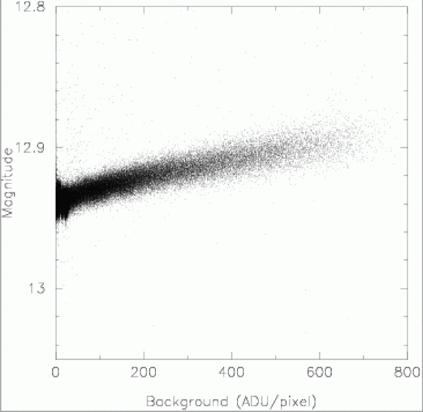
Figure 3: The relationship between the instrumental magnitude and the background level as measured on the CCD frame.

Once the instrumental photometry has been extracted, variable stray light effects must be removed. It was discovered that the background as determined in §2.2.4 level needs to be scaled to properly remove the contribution from stray light. The cause of this effect may because the 2D fits (see §2.2.4) are not sufficient. With the small number of subraster pixels a higher order polynomial is not stable enough, hence the estimation of the background level is not optimum. Regardless, it can be corrected. In Figure 3, the relationship between instrumental magnitude and the background level is shown. A fit is made between the stellar flux and the background level either with a polynomial or a cubic spline depending on the complexity of the relationship. If the relationship is modeled with a cubic spline, then the original data are binned before the fit, with 500 data points per bin and a minimum bin width of 10 ADU per pixel. In most cases the peak-to-peak amplitude of stray light variations is reduced by this approach to a few $\times$ 0.1 millimag. It can be further reduced by techniques such as subtracting a running, averaged background phased to the orbital period (Rucinski et al., 2004). The advantage of the simple approach taken here is that no prior knowledge of the orbital period is required and the amplitude of the stray light component is allowed to vary from orbit to orbit with changes in the Earth’s albedo.

3 HD 209458

3.1 Observations

Observations of HD 209458 were made during 14 - 30 August 2004, as part of a relatively short trial run on this star. This star is accessible to MOST in its Continuous View Zone (see §1) for approximately 45 days, but this was the first opportunity to test the Direct Imaging mode on an exoplanetary system target. The exposure time was 1.50 s (regulated to better than 1 $\mu$s). Sampling rates were varied. During most of the run, to stay within downlink margins for the MOST ground station network, data were collected at a rate of 5 per minute. For 15 hours centred on the predicted times of exoplanetary eclipse, the sampling rate was increased to 10 per minute. This improved our sensitivity to eclipses, while staying within the MOST on-board buffer capacity so no data would be lost in the event of a malfunction of one of the three ground stations.

There were data losses in the first third of the run due to crashes of the satellite’s control system (ACS) when subtle bugs in new software (which had operated smoothly during the previous month of observations on another target) manifested themselves. Once the problem was traced, the previous version of the software was uploaded to the satellite and observations continued with only one brief interruption due to a cosmic-ray-induced crash. The overall duty cycle of the raw photometry is about 85%.

Near the solstices, the contributions of scattered Earthshine (stray light) in the MOST focal plane reach their peak. For a bright Fabry Imaging target, the stray light can be less than 1% of the stellar signal. for a fainter Direct Imaging Target like HD 209458 (V $\sim$ 7.7), there is an interval during each orbit where the stray light is high enough to seriously degrade the quality of the photometry. Whenever the background level exceeded 300 ADU/pixel in an exposure, that measurement was excluded from the analysis. This represents about 25 minutes from each 101.413-min orbit, reducing the total duty cycle to 53% but still providing thorough coverage of the times of transit and eclipse.

There is an unfortunate coincidence between the orbital period of the HD 209458 exoplanet around its parent star and the orbital period of the MOST satellite around the Earth. The ratio of the two periods is 50.049, so that over the 2-week span of the MOST observations, the satellite orbital period maintains rough phasing with the exoplanet epheremis.

MOST was designed to be a non-differential photometer in its Fabry mode, but in the Direct Imaging, there can be other stars in the field appropriate as photometric comparisons. In the HD 209458 field, two other relatively bright stars were also monitored: HD 209346 (V = 8.33) and BD+18 4914 (V = 10.60); see Table 1. Even the brighter of these two is almost 0.7 mag fainter than HD 209458, so differential photometry tends to add noise to the point-to-point scatter and degrade the sensitivity to eclipses. However, it does provide a check for slow instrumental and/or environmental drifts. It was noticed that the data for HD 209458 during JD 1693 - 1693.5 (JD - 2451545.5) showed a slow trend that was not present in HD 209346. This change was approximately 0.005 mag. This could represent intrinsic variability in the star HD 209458a. Since we are interested in variations due to phase changes of the planet over the orbital period one cannot fit the trend and restore the data without perturbing trends due to the planet so it was excised from this analysis. This stretch of data did not overlap with a phase of transit or eclipse thus its exclusion has minimal effect for detection of the secondary eclipse.

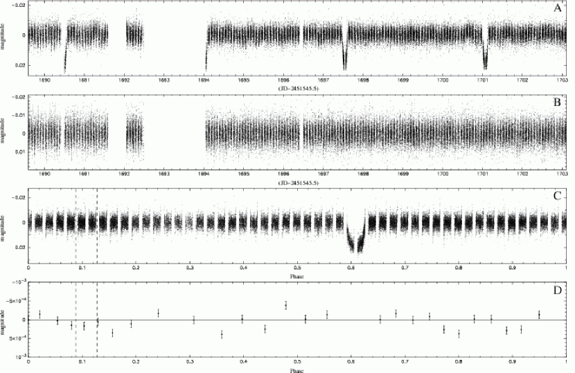
Figure 4: Panel A shows the light curve for HD 209458, panel B shows HD 209346, panel C shows data for HD 209458 phased with the planet orbital period and panel D shows the data phased with the planet orbital period and heavily binned. The dashed lines in panels A and B mark when eclipse occurs.

The reduced light curves for HD 209458 and HD 209346 are shown in Figures 4a and 4b. The primary transits in the HD 209458 system are obvious, as are the regular gaps during each satellite orbit in which data were removed due to high stray light.

Next any residuals due to the orbital period where removed from both light curves by fitting an equation of the form

$$mag=A_{0}+\sum_{j=1,n}A_{j}\cos(j\omega t+\phi_{j}),$$ (2)

where $A_{0}$ is the mean magnitude, $A_{j}$ and $\phi_{j}$ are the amplitude and phase coefficients for the cosine series. $\omega$ is ($2\pi$/period) and n=8 was chosen to accomidate the non-sinusoidal shape of the stray light residuals. Long term trends in the light curve for HD 209458 were removed by binning the comparison star with 0.2d bins and interpolating with a cubic spline. The last step was to filter a 1-cycle/day variation in the data (peak-to-peak amplitude   1.3 mmag) in the data likely due to the fact that the MOST satellite returns to a similar albedo feature on the Earth each day.

The final reduced data are presented in a phase diagram in Figure 4c, using the ephemeris for HD 209458b determined by Wittenmyer et al. (2005), with an exoplanetary period of 3.52474554 d. The ”tire-track” pattern in the data is due to the intervals of high stray light subtracted from each MOST orbit and the near-harmonic relationship between the orbital periods of the exoplanet and the MOST satellite. Unfortunately, intervals of high stray light happened in this data set to coincide with the phases of ingress, minimum and egress of the exoplanetary transits. The primary transit is obvious in Figure 4c; the range of phases of the secondary eclipse is marked in the figure.

4 Upper Limit on the Eclipse

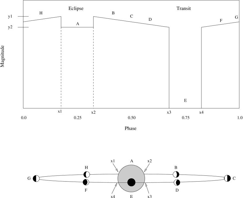
Figure 5: The eclipse model schematic. Point A marks when the eclipse is occurring and the magnitude at this point is defined at $y_{2}$. The points on ingress and egress are labeled as $x_{1}$ and $x_{2}$. As the planet moves along its orbital path the light curve proceeds through points B, C and D. When the transit occurs the total flux from the system drops and is marked as Point E. The start and finish of the transit is labeled as $x_{3}$ and $x_{4}$. The planet and light curve then proceeds through points F, G and H towards the occurrence of another transit.

To search for evidence of an eclipse in the light curve, we apply a model of the light variations due to the reflected light of the exoplanet which is shown schematically in Figure 5. We neglect any intrinsic variability of the star in this version of the model. During segment A of the phase diagram, the planet is totally eclipsed by the star, and the system has a total magnitude of $y_{2}$. As the planet moves in its orbit towards inferior conjunction at point D (middle of transit), the illuminated fraction of the planet disk decreases. The points of maximum brightness occur at phases $x_{1}$ and $x_{2}$ where the planet is almost fully illuminated; minimum brightness (outside of transit) occurs at phases $x_{3}$ and $x_{4}$, where we see the night side of the planet.

We can set up a simple model to approximate the expected phased light curve by a series of straight lines connecting the points $x_{1},x_{2},x_{3}$ and $x_{4}$. In reality these points should be connected by slowly varying curves, but our first order approximation is valid considering the star-planet flux ratio is greater than 10 000.

Thus if $x_{1}\leq x<x_{2}$ we have

$$f(x;y_{1},y_{2})=y_{2};$$ (3)

if $x_{2}\leq x<x_{3}$

$$f(x;y_{1},y_{2})=\left(\frac{y_{2}-y_{1}}{x_{3}-x_{2}}\right)(x-x_{2})+y_{1};$$ (4)

and if $x_{4}\leq x<x_{1}$

$$f(x;y_{1},y_{2})=\left(\frac{y_{1}-y_{2}}{x_{1}-x_{4}}\right)(x-x_{4})+y_{2}.$$ (5)

Since, we know a priori when are the phases of eclipse and transit, we can define $x_{1}$=0.087, $x_{2}$=0.127, $x_{3}$=0.587, and $x_{4}$=0.627. These were chosen to bracket the duration of the eclipse and transit and also reside in the gaps of the light curve where data was cut due to high levels of Earthshine with a duration of 3.4 hours ($x_{2}$ - $x_{1}$). The depth of the eclipse will be, by definition, the difference between $y_{1}$ and $y_{2}$.

We choose a Bayesian approach to directly compute the probability distribution of the eclipse depth as we descripe below. To find the most probable values for $y_{1}$ and $y_{2}$ based on the data, we start with Bayes’ Theorem

$$p(H|D,I)=\frac{p(H|I)p(D|H,I)}{p(D|I)},$$ (6)

where we have adopted the formalism of Gregory (2005). $H$ is our hypothesis of interest, $D$ is our data set, and $I$, our current state of knowledge. Starting with $p(y_{1},y_{2}|D,I)$, we obtain an expression for the probability of $y_{2}$ by marginalizing over $y_{1}$, giving us

$$p(y_{2}|D,I)=\frac{p(y_{2}|I)}{p(D,I)}\int p(y_{1}|I)p(D|y_{1},y_{2},I)dy_{1},$$ (7)

where we have chosen a Jeffrey’s Prior

$$p(y|I)=\frac{1}{y\ ln(\frac{y_{max}}{y_{min}})}$$ (8)

to give equal probability to all parameters where $y_{min}$=-0.3 mmag and $y_{max}$=0.3 for both $y_{1}$ and $y_{2}$. This where chosen based on the scatter seen in the binned phased light curve shown in Figure 4d. We repeated all calculations using a uniform prior and found no change in our results as our parameter range is well constrained by the data set. Since the dataset is well constrained it should be noted that a maximum likelihood analysis will give similar results as the probability distribution is not strongly affected by our prior. The likelihood function is given by

$$p(D|y_{1},y_{2},I) = {\rm Exp}[-\chi^{2}]\ \prod_{i=1}^{n}\frac{1}{\sqrt{2\pi}\sigma_{i}},$$ (9)

$$\chi^{2} = \sum_{i=1}^{n}\frac{(d_{i}-f(x_{i};y_{1},y_{2}))^{2}}{\sigma_{i}^{2}},$$ (10)

where $f(x;y_{1},y_{2})$ is given by Equations 3-5, , $d_{i}$ are the observations, $\sigma_{i}$ are the photometric errors for each observation, n is the number of observations and the normalization factor is

$$p(D|I)=\int\!\!\!\int p(y_{1}|I)p(y_{2}|I)p(D|y_{1},y_{2},I)dy_{1}dy_{2}.$$ (11)

Using all available data except during high levels of Earthshine we find that ($y_{2}-y_{1}$) is -0.08 $\pm$0.05 mmag (90% confidence), which would imply the system is getting brighter during the planetary eclipse. The confidence levels are plotted in Figure 6. In this analysis, we have not accounted for potential intrinsic variations in the star. To make our analysis less sensitive to longer-term variability in the star, we restricted the data set to phases bracketing the eclipse, defining three bins of equal size: one extending from $x_{1}$ to $x_{2}$ and two other bins of equal size ($x_{2}-x_{1}$) adjacent to the eclipse. Our initial choice of $x_{1}$ and $x_{2}$ to occur in the data gaps also means that the new adjacent boundaries occur at data gaps. This means that each bin will have approximately the same signal-to-noise ratio. We then recalculated the probabilities for $y_{1}$ and $y_{2}$, which we plot in Figure 7 using 1, 2 and 3 $\sigma$ confidence levels for a 2-dimensional distribution. The best fit parameter for the value of $y_{2}-y_{1}$ are then obtained from maximum of equation 7 where we have adjusted the mean of the dataset so that $y_{1}$ is equal to zero. Our detection limits are summarized in Table 2. Our fit is consistent with no detection of an eclipse, but it does allow us to place an upper limit and confidence interval on the photometric depth of the eclipse. We also repeated our analysis via a chi-squared minimization analysis. In this case one minimizes Equation 10 and we get a best fit for $y1-y2$ of 0.018 mmag. Thus our answers remain unchanged under this type of analysis as our choice of prior does not strongly affect our probability distribution.

5 Upper Limit on the Albedo of HD 209458b

In this section we derive the upper limit on the planet-star flux ratio and convert it to an upper limit on the geometric albedo.

We convert the secondary eclipse upper limit value from magnitudes to a planet-star flux ratio using the standard equation for the definition of magnitude,

$$y_{1}-y_{2}=-2.5{\rm log_{10}}\frac{F_{p}+F_{*}}{F_{*}}.$$ (12)

We take the error on the secondary eclipse $y_{1}-y_{2}$ as the eclipse upper limit, because the scatter in the data is larger than the putative eclipse measurement. Table 2 lists the upper limit (derived in §4) for different confidence levels. Here we work with the 1 $\sigma$ (or 68.3% confidence level) eclipse upper limit value, which is 0.053 mmag.

Using the eclipse upper limit $y_{1}-y_{2}=0.053$ mmag, the planet-star flux ratio upper limit is

$$\frac{F_{p}}{F_{*}}\leq 4.88\times 10^{-5}.$$ (13)

The albedo is a more intuitive form of the planet-star flux ratio, since it describes the fraction of stellar radiation that is scattered by the planet.

The geometric albedo, $A_{g}$ is the quantity relevant to the MOST measurement. $A_{g}$ is defined as the ratio of the planet’s luminosity at full phase to the luminosity from a Lambert disk with the same cross-sectional area as the planet. $A_{g}$ is equivalent to the fraction of incident stellar radiation scattered in the direction of the observer for planetary full phase (if the stellar intensity is spatially uniform). The MOST measurement occurs over a range covering 7 degrees on either side of full phase, and is close enough to full phase that we use the geometric albedo terminology. $A_{g}$ is usually specified at a particular wavelength, so we use $A_{g{\rm MOST}}$ for the geometric albedo integrated over the MOST bandpass (400 to 700 nm, see Table 3) and $A_{g{\rm TOT}}$ for the geometric albedo integrated over all wavelengths.

$A_{g}$ is related to the planet-star flux ratio by

$$\frac{F_{p}}{F_{*}}=A_{g}\left(\frac{R_{p}}{a}\right)^{2},$$ (14)

where $R_{p}$ is the planetary radius and $a$ is the semi-major axis. Taking $R_{p}=1.35\pm 0.06R_{J}$ (Brown et al. 2001) and $a=0.046$ AU (Mazeh et al. 2000), $A_{g{\rm MOST}}\leq 0.25$. The 5% uncertainty in planet radius translates into a $\sim$ 10% uncertainty in $A_{g}$. We therefore more accurately state our HD 209458b 1$\sigma$ geometric albedo upper limit as

$$A_{g{\rm MOST}}\leq 0.25\left(\frac{1.35}{R_{p}}\right)^{2}.$$ (15)

6 Discussion

HD 209458b’s geometric albedo of $\leq 0.25$ is a relatively low value. The solar system giant planet albedos in the MOST bandpass are $\gtrsim 0.4$, with Jupiter’s value 0.5 (computed from data in Karkoschka (1998); see Table 4). HD 209458b is therefore less than half as bright as Jupiter at the MOST wavelengths.

The solar system giant planets all have bright cloud decks (water ice or ammonia ice) which cause them to be bright in the MOST bandpass. HD 209458b is an order of magnitude hotter than Jupiter, far too hot for water or ammonia clouds to be present. HD 209458b may have clouds in its atmosphere, but composed of high-temperature condensates such as silicates or solid iron, instead of from ices. Clouds at high altitude are consistent with previous observations of the HD209458b atmosphere including: a primary transit low sodium absorption (Charbonneau et al., 2002); a primary transit CO non-detection (Deming et al., 2005b); and a secondary eclipse non-detection of H₂O at 2.2 $\mu$m (Richardson et al., 2003). If clouds are present in the HD 209458b atmosphere, the low $A_{g{\rm MOST}}$ rules out any bright clouds at high altitudes. Unlike ice clouds, high temperature-condensate clouds may be dark if they consist of small particles or are predominantly Fe (see Figure 5 in Seager et al. (2000)). If HD 209458b does not have clouds, strong sodium and potassium atomic absorption could be present on the day side and cause a low albedo in the MOST bandpass. While $A_{g{\rm MOST}}$ is not definitive, it is a key constraint on HD 209458b atmosphere models with specific regard to the thickness, altitude, composition, and particle size distribution of clouds. Our measurements are consistant with the results of Collier Cameron (2002) and Leigh et al. (2003) that also find low albedo upper limits for the short period planetary companions of $\upsilon$ And and HD 75289 which have orbital periods of 4.6d and 3.5d, similar to HD 209458b.

With an upper limit determined for the measured geometric albedo a natural question is can we estimate the Bond albedo? The Bond albedo, $A_{B}$, is the total radiation reflected from the planet compared to the total incident radiation, i.e. the total amount of radiation reflected in all directions integrated over all wavelengths. $A_{B}$ is an important physical parameter because it specifies the amount of stellar radiation absorbed by the planet and hence the equilibrium temperature of the planet,

$$T_{eq}=T_{*}\left(\frac{R_{*}}{2a}\right)^{1/2}\left[f(1-A_{B})\right]^{1/4},$$ (16)

where $R_{*}$ is the stellar radius, $T_{*}$ is the stellar effective temperature, $a$ the semi-major axis, and $A_{B}$ the Bond albedo. Here $f$ is the proxy for atmospheric circulation, $f=1$ if the absorbed stellar radiation is redistributed evenly throughout the planet’s atmosphere (e.g., due to strong winds rapidly redistributing the heat) and $f=2$ if only the heated day side reradiates the energy. Figure 9 shows $T_{eq}$ for the HD209458 parameters ($T_{*}=6000$ K, $R_{*}=1.18R_{\odot}$, and $a=0.046$ AU; Mazeh et al., 2000; Cody & Sasselov, 2002). The upper left corner represents our parameter range space based on 1 $\sigma$ limits.

In principle $A_{B}$ could be measured for a transiting extrasolar planet if its brightness at all phases could be measured in a wavelength range that encompasses all the planet’s scattered light. However, HD 209458 is too faint for such a measurement by MOST, and MOST’s bandpass has a cutoff at 0.7 microns (Table 3). Nevertheless, we estimate an $A_{B}$ upper limit for HD209458b, based on the solar system planet albedos, the $A_{g{\rm TOT}}$/$A_{B}$ relation, and model atmosphere considerations.

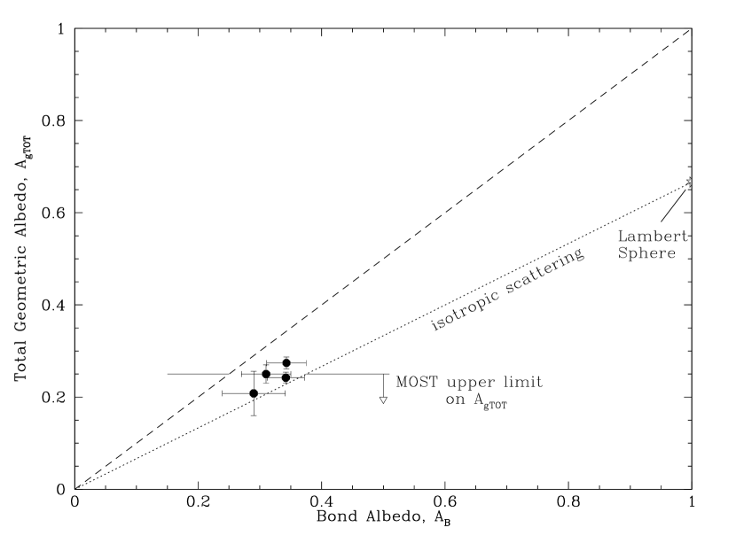
Figure 8: Relationship between the Bond albedo ($A_{B}$) and total geometric albedo ($A_{g{\rm TOT}}$) for a Lambertian sphere and solar system giant planets. The points are for Uranus, Neptune, Saturn, and Jupiter (in order of increasing $A_{B}$). The dotted line ($A_{g{\rm TOT}}/A_{B}$ = 0.67) is for Lambertian isotropic reflectance (i.e., constant for all angles of incidence). The dashed line is the line of equivalence where $A_{g{\rm TOT}}=A_{B}$ (all gas giant planets with deep atmospheres must lie to its right). The wedge between the dotted and dashed lines defines a useful limiting region: it bounds the photometric properties of most spherical bodies with deep atmospheres (with, e.g., Rayleigh scattering, clouds, dust, etc.). Hence for HD 209458b, with the assumption of $A_{g{\rm TOT}}=A_{g}{\rm MOST}$ and $A_{g{\rm MOST}}\leq 0.25$, we estimate that $A_{\rm B}\leq 0.375$.

The solar system giant planets all have $A_{B}>A_{g{\rm TOT}}$, as illustrated in Figure 8. This can be understood by considering a Lambertian planet, with $A_{B}=1.$ $A_{g{\rm TOT}}$ would have to be less than one, since $A_{g}$ includes only the radiation scattered back toward the observer. More precisely, for a Lambert sphere $A_{B}=1.5~{}A_{g{\rm TOT}}$ (Lambert’s law is the dotted line in Figure 8). Under the reasonable assumption that HD 209458b is a gas giant planet with a thick atmosphere and no reflecting surface, we can confine our attention to the very general theoretical case described by a semi-infinite atmosphere model. In this case the physically relevant albedo parameter space in Figure 8 is bound by the dashed and dotted lines, $0.67<A_{g{\rm TOT}}/A_{B}<1$ (e.g., Sobolev, 1975). Indeed, the solar system giant planet albedos comply (Conrath et al., 1989, reproduced in Table 4). Therefore, under the simplest case assumptions about the atmosphere of HD 209458b, we can use the isotropic scattering limit (dotted line) in order to derive an upper limit on its $A_{B}$. Multi-layered atmosphere models and other complications can produce geometric albedos below that limit by no more than $\sim$10% (see Sobolev (1975), Ch.9).

One further assumption is required in order to estimate HD 209458b’s $A_{B}$ from the $A_{g{\rm MOST}}$ upper limit: $A_{g{\rm TOT}}=A_{g{\rm MOST}}$. We first note that the $A_{g{\rm TOT}}<A_{g{\rm MOST}}$ for solar system planets because of strong CH₄ absorption redward of the MOST bandpass, but blueward to the wavelength where their thermal emission dominates over scattered radiation. HD 209458b is an order of magnitude hotter than the solar system giant planets and should differ. If HD209458b were a blackbody emitter, its thermal emission would peak around 2–5 microns (depending on its actual equilibrium temperature). HD209348b, however, is expected to deviate significantly from a blackbody. Near-IR molecular absorption could induce thermal emission as short a wavelength as 0.8 or 0.9 microns (see Seager et al. (2005) and references therein). In low-geometric-albedo models, the thermal emission could dominate over scattered radiation at such short wavelength and $A_{g{\rm TOT}}\simeq A_{g{\rm MOST}}$ is not too unreasonable. With $A_{g{\rm TOT}}$ and the $0.67<A_{g{\rm TOT}}/A_{B}<1$ argument (Figure 8), we estimate for HD 209458b that $A_{B}\lesssim 0.375$.

From equation (16) this value of $A_{B}$ gives $T_{eq}>1300$ K. In Figure 9 we show how this estimated $A_{B}$ value together with the Spitzer/MIPS 24 $\mu$m brightness temperature measurement of 1130 K (Deming et al., 2005b) constrain the overall $T_{eq}$ of HD209458b.

A more robust $A_{B}$ estimate requires detailed model computations, beyond the scope of this paper. Because of a wide viable parameter space (Seager et al., 2005, and references therein), however, more data are required before a definitive HD209458b model atmosphere can be computed. Indeed strong H₂O near-IR absorption has not yet been detected (Richardson et al., 2003; Seager et al., 2005). Upcoming data, including Spitzer programs for secondary eclipse thermal emission measurements (photometry from 3.5 to 8 microns and spectra from 7.4 to 14.5 microns) and HST primary transit data analysis for H₂O absorption (T. Brown 2005, private communication) will help constrain models and thus the $A_{B}$ estimate.

In summary, MOST has observed HD209458 for 14 days and we have derived an upper limit on the planet-star flux ratio of $4.88\times 10^{-5}$, corresponding to a geometric albedo of $\leq 0.25$ at the $1\sigma$ level. These numbers at the 3$\sigma$ level are $1.34\times 10^{-4}$ and 0.68 respectively. During a second HD209458b observing campaign three times longer than the one described in this paper, MOST will either detect the secondary eclipse or put a significant limit on it to a geometric albedo of 0.13 (1 $\sigma$) or 0.34 (3 $\sigma$). As the only existing constraint on scattered light from HD209458b, the MOST geometric albedo upper limit will play a pivotal role in constraining HD209458b atmosphere interpretations.

Table 1: Coordinates of Direct Imaging Target Stars.

ID	R.A.	Dec.	Mag. (V)	(B-V)	Spec. Type
HD 209458	$22^{{\rm h}}03^{{\rm m}}10.80^{{\rm s}}$	$+18\arcdeg 53^{\prime}04.0^{\prime\prime}$	7.65	0.53	G0V
HD 209346	$22^{{\rm h}}02^{{\rm m}}21.33^{{\rm s}}$	$+18\arcdeg 49^{\prime}59.2^{\prime\prime}$	8.33	0.25	A2
BD+18 4914	$22^{{\rm h}}02^{{\rm m}}37.70^{{\rm s}}$	$+18\arcdeg 54^{\prime}02.6^{\prime\prime}$	10.6	0.5	F5

Table 2: Eclipse of HD 209458b.

		Confidence Level (%)
Parameter	Best Fit	68.3	95.4	99.7
$y_{2}-y_{1}$ (mmag)	0.013	0.053	0.105	0.145
$F_{p}/F_{*}$	1.20 $\times$ $10^{-5}$	4.88 $\times$ $10^{-5}$	9.67 $\times$ $10^{-5}$	1.34 $\times$ $10^{-4}$
$A_{g}$	0.06	0.25	0.49	0.68

Table 3: MOST bandpass filter characteristics.

Wavelength	Transmission	Wavelength	Transmission	Wavelength	Transmission
(nm)	(%)	(nm)	(%)	(nm)	(%)
400	0.00	530	83.40	660	79.20
410	19.80	540	74.90	670	82.40
420	58.20	550	82.20	680	78.10
430	62.50	560	83.10	690	75.30
440	49.20	570	76.30	700	83.40
450	63.80	580	84.60	710	68.00
460	66.50	590	80.10	720	84.50
470	79.10	600	79.50	730	72.50
480	74.60	610	80.60	740	31.00
490	76.30	620	79.80	750	2.81
500	73.40	630	80.30	760	0.71
510	79.20	640	76.00	770	0.37
520	83.00	650	81.20	780	0.13

Table 4: Albedos of Giant Planets.

Planet	Geometric Albedo	Geometric Albedo	Bond Albedo
	MOST Bandpass	All Wavelengths
HD 209458b	$\leq$ 0.25	–	–
Jupiter	0.50	0.274 $\pm$ 0.013	0.343 $\pm$ 0.032
Saturn	0.47	0.242 $\pm$ 0.012	0.342 $\pm$ 0.030
Uranus	0.43	0.208 $\pm$ 0.048	0.290 $\pm$ 0.051
Neptune	0.38	0.25 $\pm$ 0.02	0.31 $\pm$ 0.04

TABLE CAPTIONS

Table 1. The parameters of targets observed during observations of the HD 209458 field. Coordinates are given in (J2000) and all measurements are from the Simbad astronomical database.

Table 2. Best fit parameters for the eclipse of HD 209458b. The confidence levels correspond to the 1,2 and 3 $\sigma$ levels accordingly. The first row gives the ranges for the fit of $y_{2}-y_{1}$ in mmag. The second row gives the corresponding flux ratio of the planet to the star for the MOST bandpass calculated using Equation 12. The third row gives the geometric albedo $A_{g}$ using Equation 14.

Table 3. Transmission values for the MOST bandpass filter. A finer grid of values is available upon request.

Table 4. Albedo of HD 209458b compared to albedos of the solar system giant planets. Solar system planet geometric albedo in the MOST bandpass computed from Karkoschka (1998) and other solar system planet albedos from Voyager, Pioneer, and ground-based measurements described in Conrath et al. (1989).

Figure 6: Confidence levels for eclipse using all data. The contours represent 68.3, 95.4 and 99.7% confidence levels.

Figure 7: Confidence levels for eclipse using only data around the occurrence of the eclipse. The contours represent 68.3, 95.4 and 99.7% confidence levels.

Figure 9: The dayside $T_{eq}$ for HD209458b as a function of $A_{B}$ for different values of $f$ (see equation 16). The approximate estimate of $A_{B}$ is shown as a vertical dashed line. The 24 $\mu$m brightness temperature of 1130 K is shown (dash-dot line)(Deming et al., 2005a) and can be considered a lower limit to $T_{eq}$ (Seager et al., 2005). The upper left quadrant is the parameter space range for HD209458b based on our 1 $\sigma$ limits.

References

- Burrows et al. (2005) Burrows, A. Hubeny, I. Sudarsky, D. 2005, ApJ, 625, L135
- Charbonneau et al. (2000) Charbonneau, D. Brown, T.M. Latham, D.W. Mayor, M. 2000, ApJ, 529, L45
- Charbonneau et al. (2002) Charbonneau, D. Brown, T.M. Noyes, R.W. Gilliland, R.L. 2002, ApJ, 568, 377
- Cody & Sasselov (2002) Cody, A. M., & Sasselov, D. D. 2002, ApJ, 569, 451
- Collier Cameron (2002) Collier Cameron, A., Horne, K., & Leigh, C. 2002, MNRAS, 330, 187
- Conrath et al. (1989) Conrath, B. J., Hanel, R. A., & Samuelson, R. E. 1989, Origin and Evolution of Planetary and Satellite Atmospheres, 513
- Deming et al. (2005a) Deming, D., Seager, S., Richardson, L. J., & Harrington, J. 2005, Nature, 434, 740
- Deming et al. (2005b) Deming, D., Brown, T. M., Charbonneau, D., Harrington, J., & Richardson, L. J. 2005, ApJ, 622, 1149
- Green et al. (2003) Green, D. Matthews, J. Seager, S. Kuschnig, R. 2003, ApJ, 597, 590
- Gregory (2005) Gregory, P.C. 2005, in Bayesian logical data analysis for the physical sciences: a comparative approach with Mathematica support, Cambridge University Press, New York, 41-65
- Henry et al. (2000) Henry, G.W. Marcy, G.W. Butler, R.P. Vogt, S.S. 2000, ApJ, 529, L41
- Ida & Lin (2004) Ida, S. Lin, D.N.C. 2004, ApJ, 604, 388
- Karkoschka (1998) Karkoschka, E. 1998, Icarus, 133, 134
- Konacki et al. (2005) Konacki, M. Torres, G. Sasselov, D. Jha, S. 2004, ApJ, 624, 372
- Leigh et al. (2003) Leigh, C., Collier Cameron, A., Udry, S., Donati, J.F., Horne, K., James, D., & Penny, A. 2003, MNRAS, 346, L16
- Matthews et al. (2004) Matthews, J.M. Kuschnig, R. Guenther, D.B. Walker, G.A.H. Moffat, A.F.J. Rucinski, S.M. Sasselov, D. Weiss, W.W. 2004, Nature, 430, 51
- Mayor& Queloz (1995) Mayor, M. Queloz, D. 1995, Nature, 378, 355
- Mazeh et al. (2000) Mazeh, T., et al. 2000, ApJ, 532, L55
- Moffat (1969) Moffat, A.F.J. 1969, A&A, 3, 455
- Press et al. (1992) Press, W.H. Teukolsky, S.A. Vetterling, W.T. Flannery, B.P. 1992, Numerical Recipes in Fortran 77 Second Edition, Cambridge University Press, 678
- Richardson et al. (2003) Richardson, L. J., Deming, D., & Seager, S. 2003, ApJ, 597, 581
- Rucinski et al. (2004) Rucinski, S.M. et al. 2004, PASP, 116, 1093
- Schneider (2005) Schneider, J. 2005, http://vo.obspm.fr/exoplanetes/encyclo/catalog-main.php
- Seager et al. (2000) Seager, S. Whitney, B.A. Sasselov, D.D. 2000, ApJ, 540, 504
- Seager et al. (2005) Seager, S., Richardson, L. J., Hansen, B. M. S., Menou, K., Cho, J. Y-K., & Deming, D. 2005, ApJ, in press
- Sobolev (1975) Sobolev, V. V. 1975, (Translation of Rasseianie sveta v atmosferakh planet, Moscow, Izdatel’stvo Nauka, 1972.) Oxford and New York, Pergamon Press (International Series of Monographs in Natural Philosophy. Volume 76), 1975. 263 p., 6213
- Vidal-Madjar et al. (2003) Vidal-Madjar, A. Lecavelier des Etangs, A. Désert, J.M. Ballester, G.E. R. Hébrard, G. Mayor, M. 2003, Nature, 422, 143
- Walker, Matthews et al. (2003) Walker, G. et al. 2003, PASP, 115, 1023
- Walker et al. (2005) Walker, G. et al. 2005, ApJ, 623, L145
- Wittenmyer et al. (2005) Wittenmyer, R.A. et al. 2005, astroph/0504579