Inflationary Potential Reconstruction for a WMAP Running Power Spectrum

Abstract:

The first year WMAP measurement of the CMB temperature anisotropy is intriguingly consistent with a larger running of the inflationary scalar spectral index than would be expected for single-field inflation. We revisit the issue of a large running spectral index, first by reexamining the evidence from the data, and then by reconstructing the inflationary potential, using an improved method based upon the Hamilton-Jacobi formulation. We note that a spectrum which runs only over 1.5 decades of $k$ space provides as good a fit to the CMB data as one which runs at all $k$, that significant evidence for running comes from multipoles $l$ near 40, and that large running gives a better fit than a flat spectrum primarily if the tensor-to-scalar ratio $r$ is large, $r\sim 0.5$, and the field values are at the Planck scale. This allows one to break the large degeneracy of potentials which would be consistent with the scalar power alone. Large running, should it be confirmed, is thus linked to a high scale of inflation and the possibility of seeing effects of tensor modes in the CMB and Planck-scale physics. Nevertheless, we show that the reconstructed inflaton potential is well-described by a renormalizable potential whose quantum corrections are under control despite the large field values.

1 Introduction

In 2003 the Wilkinson Microwave Anisotropy Probe (WMAP) released the results of its first year of high-precision measurements of the temperature anistropy of the Cosmic Microwave Background (CMB) [1]. While several anomalies of marginal statistical significance have been noted, one of the most visually striking is the trend of the spectral index of the scalar power $n_{s}$, to run toward smaller values [2], shown in figure 2. There it was determined that ${dn_{s}/d\ln k}\sim-0.1$ albeit with large error bars. Like the other anomalies, this one also remains to be proven statistically significant, since a flat spectrum is also consistent with the data. Nevertheless, since the present data have opened the door to the possibility of large running, it is interesting to explore the theoretical consequences while we continue to wait for the next WMAP data release.

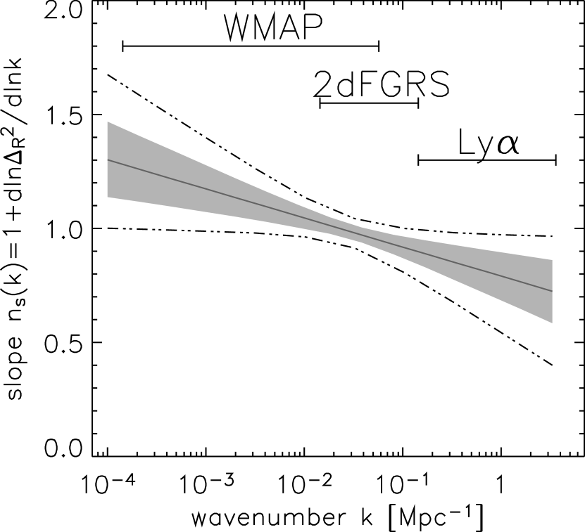
Figure 1: Experimental limit on the scale-dependent spectral index, reproduced from figure 2 of [2]. Shaded areas and dashed lines indicate 68% and 95% confidence regions, respectively.

Figure 2: Probability distribution function for running from combined WMAP and SDSS data, from [7].

It is somewhat surprising that the issue of running has not attracted as much attention as the low quadrupole since it is arguably as significant. Nevertheless there have been a number of papers which have treated running, starting even before WMAP [3]. Refs. [4, 5] were the first to examine the likelihood of a running spectrum using modern CMB and Lyman $\alpha$ data. Subsequently to WMAP, ref. [6] found that the marginal evidence for running disappeared if one omitted the first three multipoles, a conclusion which we shall challenge below. Including data from the Sloan Digital Sky Survey galaxy survey [7] slightly narrows the errors on ${dn_{s}/d\ln k}$, but not the central value, as shown in figures 2-2.

From the theoretical perspective, the $-0.1$ level of running is uncomfortably large, since ${dn_{s}/d\ln k}$ is a second order effect in the slow-roll expansion; generically one expects ${dn_{s}/d\ln k}\mathrel{\raise 1.29167pt\hbox{$<$\kern-8.50006pt\lower 4.30554pt\hbox{$\sim$}}}1/N_{e}^{2}$ with $N_{e}\sim 60$ e-foldings of inflation since horizon crossing. Ref. [8] considered which general classes of models could give large running, and methods of constructing potentials with large running. Refs. [9]-[11] showed that there is a new consistency condition between the scalar and tensor power spectra in the presence of running. Ref. [12] analyzed generically large running in conjunction with multifield inflation, and sudden changes of direction in field space. Supergravity models with two-stages of inflation have been shown to provide large running [13]. Classes of well-motivated particle physics models consistent with large running were presented in [14]; inflation in noncommutative spacetime has been found to give significant running [15, 16], as well as inflation with a cutoff on transPlanckian fluctuations [17]. In [18] it was noted that although brane-antibrane inflation models predict smaller levels of running, $dn_{s}/d\ln k\sim-0.01$, nevertheless the correlation of $dn_{s}/d\ln k$ with $n_{s}$ can provide an important test of the model if future experiments are able to reliably measure running at this low level.

One possible reason for a decline of interest in running of $n_{s}$ is that recent Lyman-$\alpha$ forest data have moved the central value much closer to zero, and narrowed the confidence intervals. Ref. [19] finds that $dn_{s}/d\ln k=-0.003\pm 0.010$ (see also [20]). This determination would seem to put the question of large running to rest. However, given the reasonable question as to whether systematic errors are completely under control in the Lyman-$\alpha$ studies, we suspend judgment until there is further confirmation from WMAP or other CMB experiments. Moreover, Lyman-$\alpha$ data are sensitive to the smallest scales. It is perfectly possible that the power spectrum runs significantly at larger scales, but flattens out at smaller scales. Indeed, this is almost a necessity since it is impossible to sustain inflation over 60 e-foldings if the running remains large throughout, as we will discuss.

There is a broader issue connected with increasingly precise experimental determinations of the inflationary power spectrum, namely, what is the shape of the inflaton potential which can generate a given spectrum [21, 22]? One of the points of this paper is that an expansion of the potential around a point using slow-roll parameters, and integrating the slow-roll approximation of the inflaton equations of motion, are inadequate for accurately reproducing the desired spectral shape, if it runs at the level which we are considering, or otherwise departs from the slow-roll approximation. In this work we present a simpler technique for reconstructing the potential, based on the Hamilton-Jacobi formulation of the inflaton equation of motion [23, 24].

We begin in section 2 with a description of the running spectrum and its likelihood, with our own analysis of CMB and large scale structure (LSS) data sets. We argue that the possibility of large running, though unproven, is still plausible, if applied to a restricted range of the power spectrum. In section 3 we describe our new method of reconstructing the potential, based on the Hamilton-Jacobi method. A one-parameter family of potentials corresponding to the running scalar power spectrum is constructed. In section 3.3 we show how higher order corrections in the slow-roll expansion for the power spectrum can be efficiently incorporated. In section 3.4 we note that a given potential yields the desired power spectrum only for a specific initial velocity for the inflaton, which does not generally correspond to the slow-roll attractor value. In section 4 we break the degeneracy between potentials found in the previous section by assuming a large tensor-to-scalar ratio, as is favored by the best fit parameters found in section 2. We discuss several aspects of this potential, including the duration of inflation which can be supported during the period of large running, and the extent to which the potential can be approximated by renormalizable terms in a quantum field theory. We give conclusions in section 5.

2 Running Power Spectrum

The power spectrum with running spectral index is parametrized as

$$P(k)=A\,\exp\left[(n_{s}-1)\ln(k/k_{0})+\frac{1}{2}{dn_{s}\over d\ln k}\ln^{2}(k/k_{0})\right]$$ (1)

The running spectrum which best fits the first year WMAP data was given in [2] with

$$n_{s}=1.27,\quad{dn_{s}\over d\ln k}=-0.1$$ (2)

at a pivot point of $k_{0}=0.002$ Mpc^-1, with a likelihood given by $-2\ln{\cal L}=\chi^{2}=1426$ for 1340 degrees of freedom (number of data points minus number of parameters). The other cosmological parameters are listed in table 1, where we show the best-fit running and nonrunning models which we obtain using the CosmoMC Markov Chain Monte Carlo program [25] (see http://cosmologist.info/cosmomc). The $\chi^{2}=1426$ value for the running spectrum includes a penalty of $\Delta\chi^{2}={1.4}$ from the high value of the Hubble parameter, $h\cong{0.814}$, relative to the Hubble Space Telescope value $h\cong 0.72$ [26]. All models shown are flat: $\Omega_{\Lambda}=1-\Omega_{m}$. We note that a sizeable tensor-to-scalar ratio $r$ (as well as a large optical depth $\tau$) is required to get the best fit with large running. If we set $r=0$ while keeping $n_{s}$ and ${dn_{s}/d\ln k}$ fixed (but allowing other cosmological parameters to vary) the likelihood decreases, $\chi^{2}=1450$. There is a degeneracy between running and tensors; if we set $r=0$ and allow all other parameters to vary, including $n_{s}$ and $dn_{s}/d\ln k$, the best fit has $\chi^{2}=1429$, but smaller running, $dn_{s}/d\ln k\sim-0.009$. Although the statistics are not yet significant, there is the hint that large running and a large tensor ratio fit the data better.

$n_{s}$	${dn_{s}\over d\ln k}$	$r$	$A$	$\Omega_{b}h^{2}$	$\Omega_{m}h^{2}$	$h$	$\tau$	$\chi^{2}/\nu$
1.27	$-0.1$	0.57	$2.1\times 10^{-9}$	0.024	0.122	0.81	0.29	1426/1340
0.99	$-$	$-$	$2.6\times 10^{-9}$	0.024	0.140	0.72	0.16	1429/1342

Table 1: Our best fits for the running and nonrunning models using CosmoMC and the first year WMAP data.

We have repeated the comparison between running and nonrunning models using data from other CMB experiments (ACBAR [27], VSA [28], CBI [29]), and galaxy surveys (2dF [30], SDSS [7]). (In all the data sets we also include the Hubble Space Telescope determination of the Hubble parameter, which contributes $156.25\times(h-0.72)^{2}$ to the $\chi^{2}$, leading to $\Delta\chi^{2}\simeq{1.4}$ between the running and nonrunning models using the WMAP data.) The best fit parameters for different combinations of these data are shown in table 2. Inclusion of other CMB data strengthen the evidence for running, while including large scale structure (LSS) data weaken the evidence. This is more evident with the inclusion of Sloan Digital Sky Survey (SDSS) data than with the 2dF data. This is consistent with the evidence for running coming principally from the low-$k$ part of the power spectrum, to which the CMB is more sensitive. If the effect turns out to be real, then the best fit to the data including large scale structure will require a spectrum which has some different behavior from eq. (1) at large $k$, as we will discuss below.

data	$n_{s}$	${dn_{s}\over d\ln k}$	$r$	$10^{9}\,A$	$\Omega_{b}h^{2}$	$\Omega_{m}h^{2}$	$h$	$\tau$	$\chi^{2}/\nu$
WMAP	1.27	$-0.10$	0.57	$2.1$	0.024	0.122	0.81	0.29	1426/1340
	0.99	$-$	$-$	$2.6$	0.024	0.140	0.72	0.16	1429/1342
CMB	1.27	$-0.095$	0.57	$2.1$	0.025	0.127	0.80	0.29	1447/1363
	0.97	$-$	$-$	$2.5$	0.023	0.131	0.74	0.14	1453/1365
2dF	1.09	$-0.047$	0.24	$2.3$	0.023	0.147	0.69	0.13	1462/1372
	0.96	$-$	$-$	$2.5$	0.023	0.142	0.69	0.11	1464/1374
CMB	1.09	$-0.051$	0.23	$2.3$	0.023	0.144	0.69	0.13	1485/1395
+2dF	0.96	$-$	$-$	$2.5$	0.023	0.140	0.71	0.11	1488/1397
SDSS	1.09	$-0.039$	0.24	$2.3$	0.023	0.153	0.68	0.14	1456/1359
	0.99	$-$	$-$	$2.6$	0.024	0.160	0.67	0.13	1454/1361
mpk	1.09	$-0.036$	0.24	$2.3$	0.024	0.155	0.68	0.14	1490/1391
	0.99	$-$	$-$	$2.6$	0.024	0.152	0.69	0.15	1490/1393
CMB	1.09	$-0.045$	0.23	$2.3$	0.023	0.148	0.68	0.14	1517/1414
+mpk	0.96	$-$	$-$	$2.5$	0.023	0.149	0.68	0.09	1517/1416

Table 2: Best fit parameters for both running and nonrunning spectral index models from CosmoMC. The first row is the result from the first year WMAP data alone; others are from the combinations of the WMAP data and the data sets specified at the first column, where CMB=ACBAR+CBI+VSA, mpk=2dF+SDSS. We used the July 2005 version of CosmoMC, and its default data sets. They are: the first year WMAP data, $2\leq l_{\rm TT}\leq 900$, $2\leq l_{\rm TE}\leq 450$ (1348 data points); July 2002 ACBAR data [27], $900\leq l\leq 1950$ (7 data points); 2000 and 2001 CBI data [29], $700\leq l\leq 1760$ (8 data points); Feb 2004 VSA data [28], $640\leq l\leq 1700$ (8 data points); June 2002 2dF data [30], 32 data points; Oct 2003 SDSS data [7], $0.016\leq k(h/{\rm Mpc})\leq 0.205$ (19 data points).

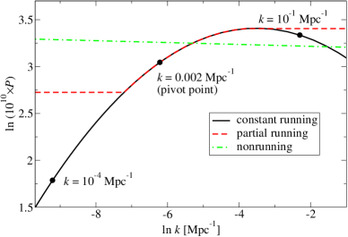
Figure 3: Log of best fit running spectrum (solid, black) and the partial running spectrum (dashed, red) versus $\ln k$. The nonrunning spectrum is also shown (dot-dashed, green).

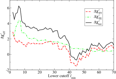
Figure 4: Difference of $\chi^{2}$ between the nonrunning and running models, versus the minimum multipole included $l_{\rm min}$; see eq. (2.3). The separate contributions from temperature (TT) and polarization (TE) as well as the total are shown.

The relevant part of the spectrum is shown in figure 4; the range of $k$ values here is that which is actually called by the CAMB program (see http://camb.info/) in computing the multipole moments of the temperature anisotropy and polarization of the WMAP data. The scales $k=10^{-4}$ Mpc^-1 and $k=10^{-1}$ Mpc^-1 indicated on figure 4 correspond roughly to the quadrupole and the $l=2000$ mode of the multipoles of the acoustic peaks. It is interesting to note that the first year WMAP data are equally consistent with both curves shown in figure 4; the solid one having a constant value of $dn_{s}/d\ln k$, and the dashed one having ${dn_{s}/d\ln k}=0$ outside of the range ${-7.2}<\ln(k\cdot{\rm Mpc})<{-3.8}$. Both of these spectra have the same likelihood, even without varying the cosmological parameters given in table 1. We have verified this using our modified versions of CAMB and CosmoMC which allow for an arbitrary user-specified power spectrum. We will make further use this truncated version of the running spectrum, which is flat at large and small $k$, referring to it as the partial running model.

It is at first surprising that the partial running model should provide as good a fit to the data as the constant running model, since [6] showed that the evidence for running comes mainly from the lowest three multipoles. In contrast the running part of our partial running spectrum affects much higher multipoles. To better understand this, we have computed the difference in $\chi^{2}$ between the nonrunning and running models including contributions from $l_{\rm min}$ to $l_{\rm max}$ (900 for TT and 450 for TE):

$$\Delta\chi^{2}(l_{\rm min})=\sum_{l=l_{\rm min}}^{l_{\rm max}}\delta\chi^{2}(\rm nonrunning)-\delta\chi^{2}(\rm running)$$ (3)

where $\delta\chi^{2}(l)$ is the $\chi^{2}$ contributed from diagonal ($l$) and off-diagonal $(l^{\prime}>l)$ terms. This is shown in figure 4. We observe there that the low multipoles ($l=2,3,4$) in the TT data do account for a substantial part of the total decrease in $\chi^{2}$ between the nonrunning and running models; however the TE data, ignored by the analysis of [6], have the opposite effect and hence the $\Delta\chi_{\rm tot}^{2}$ is rather insensitive to the inclusion of the first three multipoles. In fact, the larger part of the decrease in $\chi^{2}$ clearly comes from the region near $l=40$ in the TT data, which explains why our partial running spectrum starts running at relatively high $k$ values, $k\cong 0.001$ Mpc^-1, compared to the the values which would affect the low multipoles, $k\cong 10^{-4}$ Mpc^-1. This perspective lends more interest to the possible confirmation or negation of large running by future improvements in the data, since the experimental determination of the higher multipoles is not so limited by cosmic variance.

Although the LSS data do not favor the running models as shown in table 2, we have also looked for the best fit models using the partial running spectrum, where we allowed the low and high $k$ values which define the partial running model to vary. Table 3 shows the best fit values and the likelihood for the different data sets. Since other CMB data strengthen the evidence for running, but LSS data weaken it, when including LSS data, the lower cutoff will be larger than, and the higher cutoff will be smaller than, those including other CMB data. All the $\chi^{2}$ values for the partial running model are seen to be lower than or equal to the running and nonrunning models.

	WMAP	CMB	2dF	CMB+2dF	SDSS	mpk	CMB+mpk
$\ln k_{\rm low}$	$-7.2$	$-7.1$	$-6.5$	$-6.4$	$-6.5$	$-6.5$	$-6.5$
$\ln k_{\rm high}$	$-3.8$	$-2.4$	$-2.8$	$-2.4$	$-2.8$	$-2.7$	$-2.6$
$\chi^{2}$	1426	1447	1462	1485	1454	1488	1514

Table 3: The likelihood of the partial running model, using the data described in table 2.

To summarize our view of the experimental evidence: there is an interesting hint of a running spectrum which is driven in large part by multipoles near $l=40$ in the CMB data; the inclusion of large scale structure data do not reinforce this, but they also do not contradict it. Although the statistical significance is not great, it can also be argued that it is not negligible. According to the Bayesian information criterion [31], one should decide whether the addition of new parameters is justified by considering whether the combination

$$BIC=\chi^{2}+k\ln N$$

is decreased, where $k$ is the number of parameters and $N$ is the number of independent data points. Not all multipole moments of the CMB should be considered as independent, since it is known that the acoustic peaks can be fit with great accuracy by a Fourier series with 20 terms. A change of $\chi^{2}$ of $3$ can therefore support $3/\ln 20\cong 1$ new parameters. Although we introduced two new parameters, the running and the tensor-to-scalar ratio, there is a degeneracy between these, which makes them more like one parameter. The effect we are discussing is therefore on the borderline of being significant, a situation that could change in either direction with new data.

3 Reconstruction of Potential

3.1 Formalism

To find inflaton potentials corresponding to a desired power spectrum, the Hamilton-Jacobi formulation of inflation is useful [23, 24]. Here we introduce a method based on integration over $H(k)$, which is simple and accurate; see ref. [32] for more discussion and results in constant spectral index case. Ref. [21] presented a similar integration method, but used the lowest order slow-roll approximation in each step, and hence their method is not as accurate as Hamilton-Jacobi formulation which we describe. Initially, one takes the Hubble parameter to depend on the inflaton field, $H=H(\phi)$. In units where $M_{\rm Pl}=1$, the Friedmann equation can be written

$$3H^{2}-2H^{\prime 2}=V$$ (4)

where $H^{\prime}=dH/d\phi$. The inflaton velocity is given by

$$\dot{\phi}=-2H^{\prime}$$ (5)

We begin by using the lowest order prediction for the power spectrum of the curvature (scalar field) perturbation in the slow-roll approximation:

$$P(k)={H^{4}\over c_{1}\dot{\phi}^{2}}$$ (6)

where $c_{1}=4\pi^{2}$, and the $k$ dependence is implicitly defined using the horizon crossing condition,

$$k/a=H\ \longrightarrow\ \ln k=\ln a+\ln H$$ (7)

Since, using (5), $\ln a=\int^{t}dtH=\int^{\phi}d\phi H/\dot{\phi}=-\frac{1}{2}\int^{\phi}d\phi\,H/H^{\prime}$ , one can take $d/d\phi$ of eq. (7) to obtain a first order differential equation determining $k(\phi)$:

$${d\ln k\over d\phi}={H^{\prime}\over H}-{H\over 2H^{\prime}}$$ (8)

Our strategy for reconstructing the potential is to rewrite the above equations using $\ln k$ as the independent variable instead of $\phi$. By straightforward manipulation using the chain rule, and eliminating $\dot{\phi}$ from eqs. (5-6), we find that

$$H^{{\phantom{|}{}^{\phantom{|}}}^{\!\!\!\!\!\!\!\!\!\circ}}\equiv{dH\over d\ln k} = -{H^{3}\over{2c_{1}}P-H^{2}}$$

$$\phi^{{\phantom{|}{}^{\phantom{|}}}^{\!\!\!\!\!\!\!\circ}}\equiv{d\phi\over d\ln k} = \pm\left[-{2H^{{\phantom{|}{}^{\phantom{|}}}^{\!\!\!\!\!\!\!\!\!\circ}}\over H}\left(1-{H^{{\phantom{|}{}^{\phantom{|}}}^{\!\!\!\!\!\!\!\!\!\circ}}\over H}\right)\right]^{1/2}=\pm\frac{2H\sqrt{c_{1}P}}{2c_{1}P-H^{2}}$$ (9)

and we choose the plus sign throughout this paper. This choice of sign has no physical significance during any period when $\phi$ is changing monotonically with time, as during inflation. These equations can be integrated numerically to find $H$ and $\phi$ as functions of $\ln k$. This implicitly defines $H(\phi)$, which can then be used in (4) to find $V(\phi)$. There is one relevant constant of integration $H_{0}$, the initial value of $H$, which determines the overall inflationary energy scale. The initial value of $\phi$ has no physical importance. For example we can take $\phi=0$ when $k$ is at the pivot point $k_{0}$ at which the power spectrum is normalized in (1).

In the following, it is convenient to refer to rescaled variables. We define a rescaled power spectrum

$$P=A{\cal P}$$ (10)

where $A$ is the amplitude of the spectrum in eq. (1), and thus ${\cal P}$ is the exponential factor ${\cal P}=\exp[(n_{s}-1)\ln{k\over k_{0}}+\frac{1}{2}\frac{dn_{s}}{d\ln k}\ln^{2}\frac{k}{k_{0}}]$. $A$ is determined by the COBE normalization, which gives $P(k_{c})=25/4\times(1.91\times 10^{-5})^{2}\simeq 2.3\times 10^{-9}$ at $k_{c}=7.5a_{0}H_{0}\simeq 0.002{\rm Mpc}^{-1}$, consistent with the values in table 1. We further rescale

$$H=\alpha{\cal H};\quad\alpha^{2}=2c_{1}{A}$$ (11)

The equations of motion become

$${\cal H}^{{\phantom{|}{}^{\phantom{|}}}^{\!\!\!\!\!\!\!\!\!\circ}} = -{{\cal H}^{3}\over{\cal P}-{\cal H}^{2}}$$

$$\phi^{{\phantom{|}{}^{\phantom{|}}}^{\!\!\!\!\!\!\!\circ}} = {{\cal H}\,\sqrt{2{\cal P}}\over{\cal P}-{\cal H}^{2}}$$ (12)

Similarly, we define the rescaled potential through

$$V=\alpha^{2}{\cal V}=\alpha^{2}\left[3{\cal H}^{2}-2{({\cal H}^{{\phantom{|}{}^{\phantom{|}}}^{\!\!\!\!\!\!\!\!\!\circ}}/\phi^{{\phantom{|}{}^{\phantom{|}}}^{\!\!\!\!\!\!\!\circ}})}^{2}\right]=\alpha^{2}{\cal H}^{2}\left(3-\frac{{\cal H}^{2}}{\cal P}\right)$$ (13)

The Hamilton-Jacobi slow-roll parameters are

$$\epsilon = 2\left({H^{\prime}\over H}\right)^{2}$$ (14)

$$\eta = 2\left({H^{\prime\prime}\over H}\right)$$ (15)

From eqs. (5 - 6), we can rewrite the $\epsilon$ as

$$\epsilon={{\cal H}^{2}\over{\cal P}}$$ (16)

Since $\epsilon<1$ is required for accelerated expansion, ${\cal H}^{2}$ is always smaller than ${\cal P}$ during inflation, so the equations of motion (3.1) remain nonsingular.

3.2 Reconstructed Potentials

The method described above can be used to numerically determine a family of potentials $V(\phi)$ which give rise to a desired scalar power spectrum $P(k)$. There is no unique potential for a given $P(k)$ since changing the scale of inflation can be compensated by a change of the slope of the potential. This can be seen through the relation $P\sim V^{3}/V^{\prime 2}$. Later on we will break this degeneracy by invoking information about the tensor power spectrum.

As a first step, we reconstruct the potentials only over the region of field space traversed by the inflaton during the first $\sim 8$ e-foldings of inflation after horizon crossing, since this is the relevant period for affecting the CMB. We numerically integrated the equations (3.1) subject to the initial conditions ${\cal H}={\cal H}_{0}$, $\phi=0$. To reproduce the spectrum shown in figure 2, we take the initial value of $\ln k_{i}=-11.8$, which corresponds to times several e-foldings before horizon crossing, and integrate to a final value of $\ln k_{f}=-1.4$. The derived potentials, and the range over which $\phi$ changes, depend strongly on the choice of ${\cal H}_{0}$. However, fairly universal behavior can be seen by graphing the function

$$\widetilde{\cal V}(\phi)={{\cal V}(\phi/\phi_{\rm f})-{\cal V}_{\rm f}\over{\cal V}_{\rm i}-{\cal V}_{\rm f}}$$ (17)

where $\phi_{\rm f}$ is the final value of $\phi$, and ${\cal V}_{\rm i,f}$ are respectively the initial and final values of ${\cal V}$, which is a monotonically decreasing function. This is shown in figure 6. The rather narrow range of potential shapes shown are actually inclusive, since potentials with smaller values of ${\cal H}_{0}$ are very close to the curve for ${\cal H}_{0}=0.01$, while the largest possible value of ${\cal H}_{0}$ (given by $\sqrt{{\cal P}{(k_{i})}}\cong 0.215$ using the spectrum (1)) yields a potential nearly coinciding with that of ${\cal H}_{0}=0.2$. Notice that ${\cal H}_{0}$ is not allowed to exceed ${\cal P}(k_{i})$ in (3.1). This traces back to the physical restriction that the Hubble parameter can never increase during inflation, or equivalently, the kinetic energy of the scalar field cannot be negative.

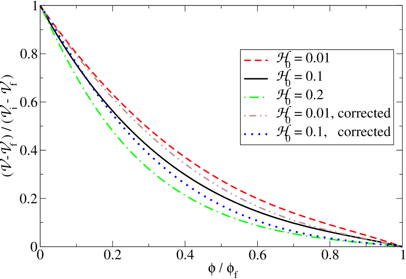
Figure 5: Reconstructed potentials for a range of initial Hubble parameters. “Corrected” curves are discussed in section 3.3.

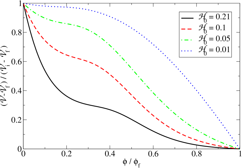
Figure 6: Reconstructed potentials of different initial Hubble parameters, integrating over 20 e-foldings of inflation.

A much greater variation in the shapes of the rescaled potential can be observed if we insist on maintaining the running index power spectrum over a longer period of inflation, going beyond that which affects the observable multipoles of the CMB temperature fluctuations. Figure 6 shows that the relative shapes of inflaton potential in different initial conditions ($\ln k_{i}=-11.8$, $\ln k_{f}=8.8$). We can see that they are quite different, but all of them have a “bump.” (Potentials with ${\cal H}_{0}$ smaller than 0.01 are close to the curve of ${\cal H}_{0}=0.01$.)

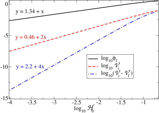
Figure 7: Dependence of potential parameters $\phi_{\rm f}$, ${\cal V}_{\rm i}$, and $({\cal V}_{\rm i}-{\cal V}_{\rm f})$, on the initial Hubble constant. Equations are numerical fits to the small-${\cal H}_{0}$ parts of the curves.

Although the relative shape of the inflaton potential is somewhat insensitive to ${\cal H}_{0}$ (at least over shorter periods of inflation), the scales over which it changes do depend strongly on ${\cal H}_{0}$. The dependences

$$\phi_{\rm f}\sim{\cal H}_{0};\quad{\cal V}_{\rm i}\sim{\cal H}_{0}^{2};\quad{\cal V}_{\rm i}-{\cal V}_{\rm f}\sim{\cal H}_{0}^{4}$$ (18)

are shown in figure 7. These dependences can be understood from equations (4-6). Since $P(k)$ does not vary, eq. (6) implies the scaling $H^{\prime}\sim H^{2}$. Thus eq. (5) predicts that $\phi$ changes by an amount $\Delta\phi\sim H^{2}\Delta t\sim H$, since we are interested in time scales of order $1/H$. Eq. (4) obviously predicts that the magnitude of $V$ scales like $H^{2}$. The variation in $V$ is $\Delta V\sim V^{\prime}\Delta\phi\sim HH^{\prime}\Delta\phi\sim H^{4}$.

The numerical value of ${\cal H}_{0}$ has no physical significance except in comparison to the value of $\sqrt{{\cal P}}$ at the chosen starting time (i.e., starting value of $\ln k$). Suppose we evolve the system for two different initial conditions, $(\ln k_{1},\ {\cal H}_{1})$ and $(\ln k_{2},\ {\cal H}_{2})$ with $k_{1}<k_{2}$. Given the solution for $(\ln k_{1},\ {\cal H}_{1})$, it is always possible to find $(\ln k_{2},\ {\cal H}_{2})$ such that the two solutions match in the region where they overlap. However the converse is not true. This is because of the attractor nature of inflationary solutions: since the effects of variation of initial conditions are exponentially suppressed with time, it is not generally possible to find initial conditions at very early times which match an arbitrary deviation from slow-roll behavior at later times. This point is important if inflation did not start much earlier than horizon crossing, so that the transient effects of initial conditions can be visible in the low-$k$ part of the power spectrum, as we will discuss in section 3.4.

3.3 Slow-Roll Corrections

In the previous subsections we reconstructed the potential using the leading slow-roll approximation for the power spectrum. Here we show how corrections which are subleading in the slow-roll expansion can be incorporated in a simple way. The next order result in the slow-roll approximation is [34]

$${\cal P}^{(2)}(k)=\left[1-\epsilon+(2-\ln 2-\gamma)(2\epsilon-\eta)\right]^{2}{\cal P}^{(0)}\equiv{\cal C}\,{\cal P}^{(0)}$$ (19)

where $\gamma\simeq 0.5772$ is the Euler-Mascheroni constant, ${\cal P}^{(0)}$ is the lowest order power spectrum which we already computed. To incorporate these corrections, which are dominated by $\eta$, we make the replacement ${\cal P}\to{{\cal P}/{\cal C}}$ in eqs. (3.1), where the correction factor ${\cal C}$ is computed using the previously obtained solution for ${\cal H}$. This procedure can be iterated until the solution converges. Convergence to a self-consistent solution is obtained after three iterations. In this way we avoid having to solve a higher order differential equation for ${\cal H}$. The second derivatives ${\cal H}^{{\phantom{|}{}^{\phantom{|}}}^{\!\!\!\!\!\!\!\!\!\!\!\circ\;\!\circ}}$, $\phi^{{\phantom{|}{}^{\phantom{|}}}^{\!\!\!\!\!\!\!\!\!\circ\;\!\circ}}$ in $\eta$ can be computed in terms of ${\cal H}^{{\phantom{|}{}^{\phantom{|}}}^{\!\!\!\!\!\!\!\!\!\circ}}$, $\phi^{{\phantom{|}{}^{\phantom{|}}}^{\!\!\!\!\!\!\!\circ}}$ using the equations of motion (3.1). The result is that the shapes (and magnitudes) of the potentials are slightly modified, as shown by the “corrected” curves in figure 6. The maximum value of ${\cal H}_{0}$ is also reduced from $0.21$ to $0.11$. The changes to the parameters in figure 7 are so slight that we do not show them.

3.4 Sensitivity to Initial Conditions

Once the potential has been determined, the power spectrum does not uniquely follow. One must also supply the initial velocity of the inflaton field. Normally this is unimportant since the inflaton reaches the attractor solution in which the slow-roll approximation $3H\dot{\phi}=-V^{\prime}$ is satisfied, hence $\dot{\phi}$ is determined by the potential. However the initial velocity required to match the desired power spectrum does not generally coincide with $-V^{\prime}/3H$; instead it is given by eq. (6).

The effect is most pronounced for large values of ${\cal H}_{0}$, as illustrated in figure 8. In this example, (where $\ln k_{i}=-9$ and ${\cal H}_{0}=0.55$, and we do not include slow-roll corrections) the initial value of $\dot{\phi}$ implied by eq. (6) is $\dot{\phi}=0.76$ (in Planck units), while the slow-roll value is $\dot{\phi}=0.33$. Using the latter value, the spectrum is distorted in its shape at the beginning of inflation, and by a constant horizontal shift $\Delta\ln k$ thereafter. The figure shows that compensating for $\Delta\ln k$ causes the two spectra to match well once the transient effect of the initial condition has died away. For smaller inflationary scales (small ${\cal H}_{0}$), the shift $\Delta\ln k$ becomes negligibly small, while the low-$k$ distortion remains significant. Since the horizon-crossing condition is that $\ln k=\ln a+\ln H$, this shift in $\ln k$ can be absorbed in a change of the scale of inflation.

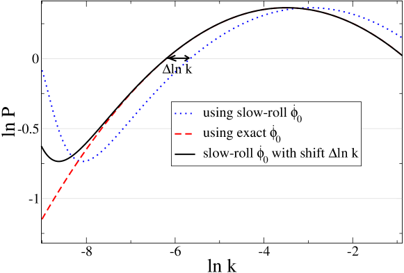
Figure 8: Power spectra obtained from reconstructed potential, for different initial conditions of $\dot{\phi}$.

4 Tensor Contribution to CMB

It was noted in section 2 that the power spectrum with large running provides a good fit to the data only if a large tensor component is also allowed. A degeneracy between these parameters is understandable, since large running suppresses power at low $k$, while the tensor contribution enhances it. In single-field inflation, which we are assuming, the tensor power is related to the scalar power, since at lowest order in the slow-roll approximation,

$$P_{t}(k)={8\over c_{1}}H^{2}$$ (20)

(compare to the scalar power, eq. (6)). This convention for the normalization of $P_{t}$ is consistent with the definition of the tensor-to-scalar ratio $r$ used by CAMB and by ref. [2],

$$r={P_{t}(k_{0})\over P(k_{0})}=16\epsilon(k_{0}).$$ (21)

Parameterizing the scalar spectrum as eq. (1) and using the WMAP parameters in table 2, we can determine the tensor spectrum as well as the reconstructed potential uniquely. However, a problem arises with the running spectrum when we try to achieve a large tensor ratio $r\cong 0.5$ at the given pivot point $k_{0}$. Namely, eq. (21) shows that $\epsilon\sim 1/32$ at $k_{0}$; however if we try to evolve backwards in time from this point using the running spectrum, the slow-roll parameters diverge, and prevent us from extending the initial value of $\ln k$ to as small values as desired. This behavior is illustrated in figure 10, which shows the reconstructed slow-roll parameters corresponding to the WMAP running spectrum. The figure shows that $\epsilon$ remains small ($<0.05$) from $\ln k\simeq-7.2$ to $1.3$, $\eta$ runs linearly and gives the running of the power spectrum. But demanding a large tensor-to-scalar requires the slow-roll parameters to be quite large at the lower scales near $k\sim 10^{-4}{\rm Mpc}^{-1}$. Moreover, negative running at large $k$ makes the power spectrum decrease exponentially, again leading to an increase in the slow-roll parameters, since $\epsilon={\cal H}^{2}/{\cal P}$. The slow-roll approximation breaks down before the end of inflation. For example, we get only 15 e-foldings while $\epsilon<0.2$ in the WMAP running model. These observations are consistent with ref. [10], who noted that $\epsilon$ reaches a minimum near the scale where $n_{s}$ crosses 1 in models with large running.

To alleviate the above problem, and extend the duration of inflation before the pivot point, we use the partial running spectrum with a low-$k$ cutoff which was discussed in section 2, and shown (together with the constructed tensor spectrum) in figure 10. We could also include the high-$k$ cutoff on the running, but we choose to omit it, in order to discuss the constraints which arise on the length of inflation if the spectrum continues to run at high $k$. The tensor spectrum is not a constant as is usually assumed when computing the CMB temperature anisotropy, and we have modified CosmoMC to use the constructed tensor spectrum. However, we do not observe any effect on the likelihood of the best fit running spectrum, nor any change in the other cosmological parameters, relative to the standard form of the tensor spectrum.

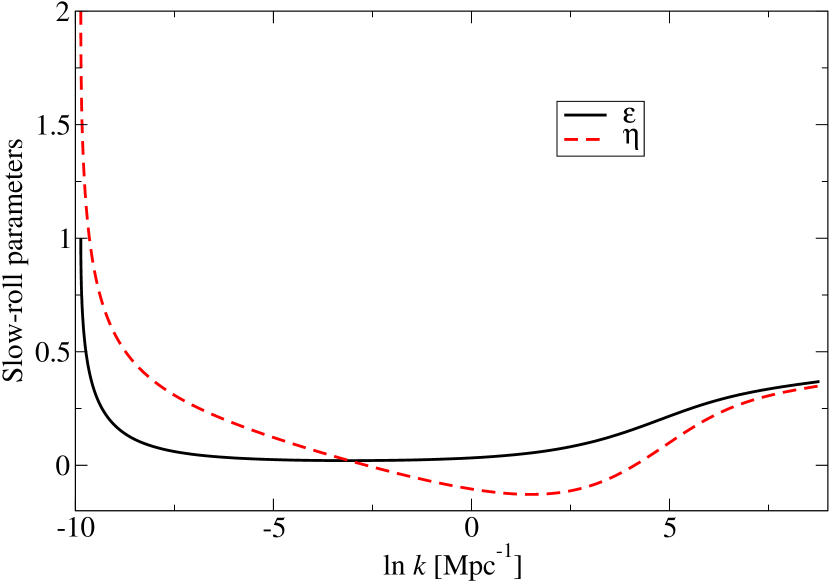
Figure 9: The reconstructed slow-roll parameters for WMAP running power spectrum, showing singular behavior at low $k$.

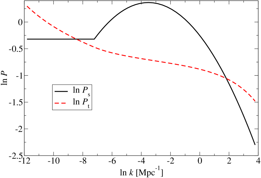
Figure 10: The partial running scalar spectrum and the reconstructed tensor spectrum (unnormalized, $A=1$).

With the low-$k$ cutoff on the running of the spectrum, the beginning of inflation can be pushed back before horizon crossing, while maintaining a large tensor ratio at the pivot point; this is shown in figure 11, where the slow-roll parameters are seen to remain small during the relevant part of inflation, while the minimum value of $\epsilon$ is consistent with $r\cong 0.5$. The discontinuity in $\eta$ is due to the discontinuity in the slope of the power spectrum where it goes between nonrunning and running, which could be avoided by making a smoother transition. On the other hand, since we chose not to cut off the running at high $k$, there is a limit on the amount of inflation after horizon crossing. The reconstructed potential continues to decrease monotonically, so there is no abrupt end to inflation, but $\epsilon$ becomes steadily larger, and quasi-exponential inflation crosses over to power-law inflation with a small power. This model gives 16 e-foldings of exponential inflation, during which $\epsilon<\epsilon_{i}=0.12$. The transition to reduced acceleration is shown in figure 13, where one can see a break in the logarithm of the scale factor versus time at around $\ln a=20$ e-foldings. Figure 13, which plots $\ln a$ versus $\ln t$, shows that after the break the expansion is indeed power-law.

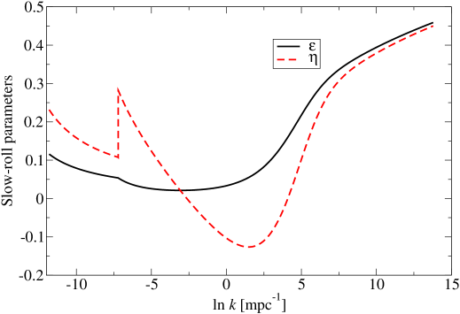
Figure 11: The reconstructed slow-roll parameters for partial running power spectrum.

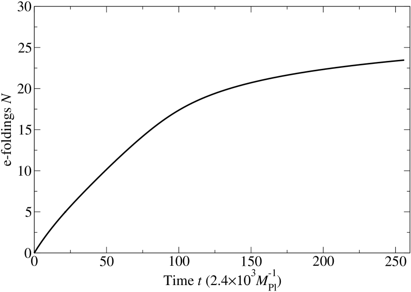
Figure 12: The logarithm of the scale factor as a function of time, showing the transition from exponential inflation to power-law expansion.

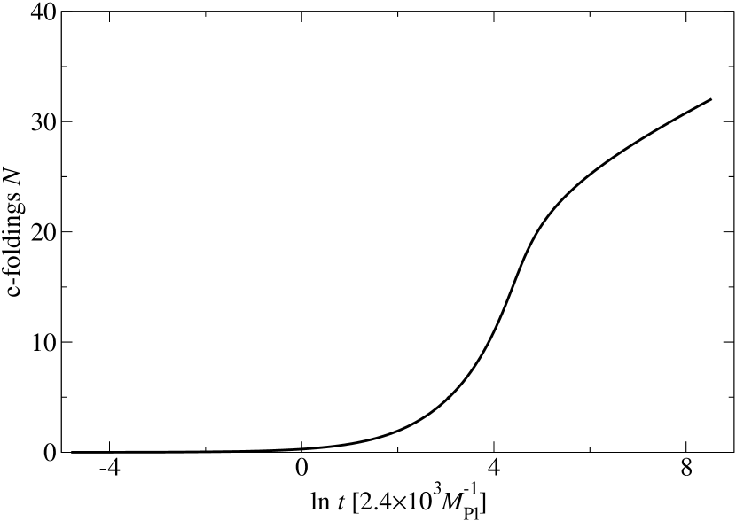
Figure 13: Same as figure 12, but plotting $\ln a$ versus $\ln t$, to show the power-law character of the expansion at late times.

With the given tensor ratio, we can uniquely determine the scale of inflation and the single out one reconstructed potential from the family that was derived in section 3.2. Members of this family were parametrized by the ratio

$${{\cal H}_{0}^{2}\over{\cal P}}={{H^{2}}\over 2c_{1}\,P}=\frac{1}{16}{P_{t}\over P}={r\over 16}={\epsilon}$$ (22)

evaluated at the initial value of $\ln k$ (not the pivot point). Figure 11 shows that $\epsilon\cong 0.12$ at the initial value $\ln k_{i}\cong-11.8$, in order to get a large enough tensor ratio at the pivot point. We find that ${\cal H}_{0}\cong 0.29$, which satisfies the constraint ${\cal H}^{2}\leq{\cal P}$ in the model with the partial running spectrum. We can then determine the scale of inflation; from table 1, $A=2.1\times 10^{-9}$, we obtain $\alpha=\sqrt{2c_{1}A}\simeq 4.1\times 10^{-4}M_{\rm Pl}\simeq 9.9\times 10^{14}{\rm GeV}$ (see eq. (11)). This corresponds to a Hubble scale of $H=\alpha{\cal H}_{0}=2.9\times 10^{14}$ GeV at the beginning of inflation, and an energy scale of $V^{1/4}=(3H^{2}M_{\rm Pl}^{2})^{1/4}=3.5\times 10^{16}$ GeV. This is the energy scale expected in the slow-roll approximation with $\epsilon\simeq 0.1$, $V^{1/4}\simeq 0.027\epsilon^{1/4}M_{\rm Pl}\simeq 3.7\times 10^{16}$GeV. The reconstructed Hubble parameter and potential, as functions of $\phi$, are shown in figures 15 and 15, where we contrast the predictions of the leading order slow roll approximation and those including corrections at second order in the slow-roll parameters. The corrections are seen to be a small effect.

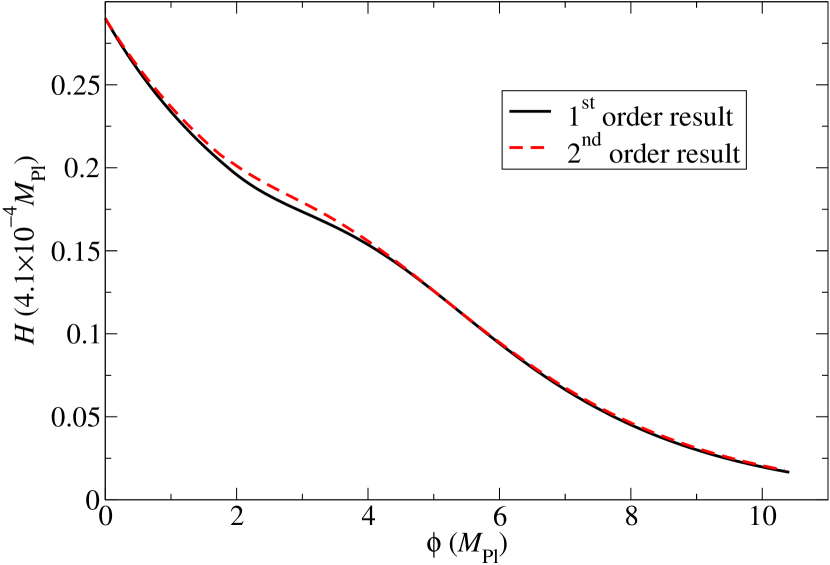
Figure 14: The reconstructed Hubble parameter, at first and second order in the slow-roll approximation, for the partial running spectrum.

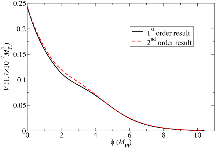
Figure 15: The reconstructed potential, at first and second order in the slow-roll approximation, for the partial running spectrum.

The reconstructed potential shows the “bump” which is characteristic of models with large running from blue ($n>1$) to red ($n<1$), since a large third derivative of the potential is required to get large running in the slow-roll prediction,

$${dn_{s}\over d\ln k}=-2\xi_{\rm V}+16\epsilon_{\rm V}\eta_{\rm V}-24\epsilon_{\rm V}^{2}$$ (23)

in terms of the usual potential slow-roll parameters: $\epsilon_{\rm V}=\frac{1}{2}(V^{\prime}/V)^{2}$, $\eta_{\rm V}=V^{\prime\prime}/V$, and $\xi_{\rm V}=V^{\prime}V^{\prime\prime\prime}/V^{2}$. From the perspective of particle physics model-building, it is interesting to ask to what extent this potential can be matched by a renormalizable potential. We have therefore fit the reconstructed $V$ to a quartic polynomial. Obviously the fit becomes better as one restricts the range of the field, so we have done this exercise for a series of final $\phi$ values, which correspond to different maximum wave numbers in the spectrum. We made our fits using $\ln k_{i}=-9.2$ ($10^{-4}$ Mpc^-1) to $\ln k_{f}=0$ (1 Mpc^-1), 3.8, 4.8, and 5.8, obtaining fits which for the case of $\ln k_{f}=4.8$ has the form

$$V=1.7\times 10^{-7}\times(0.277-0.163\,\phi+0.0583\,\phi^{2}-0.0102\,\phi^{3}+0.00064\,\phi^{4})$$ (24)

where all coefficients (and $\phi$) are in Planck units. Figure 17 plots the approximate fits against the actual reconstructed potential. Plotted in this way, all the fits look very good, but to better discriminate, we show the fractional deviations $\Delta V/V$ and correlation coefficients between the fits and the actual potential in figure 17. We see that final $k$ values up to $\ln k_{f}=4.8$ provide good fits at the percent level. This $\ln k_{f}$ value corresponds to the first 18 e-foldings of inflation. The difficulty of sustaining $50-60$ e-foldings of inflation with large running has been noted previously [8]. Our analysis gives further support to the idea that large running requires some significant change in the potential after the first few e-foldings, such as can occur in multifield models [12, 13]. It is also noteworthy in our reconstruction that the inflaton changes by superPlanckian values during this initial period of inflation. However, the smallness of the coefficients in the potential indicate that the effective field theory description is not invalidated by the large field values.

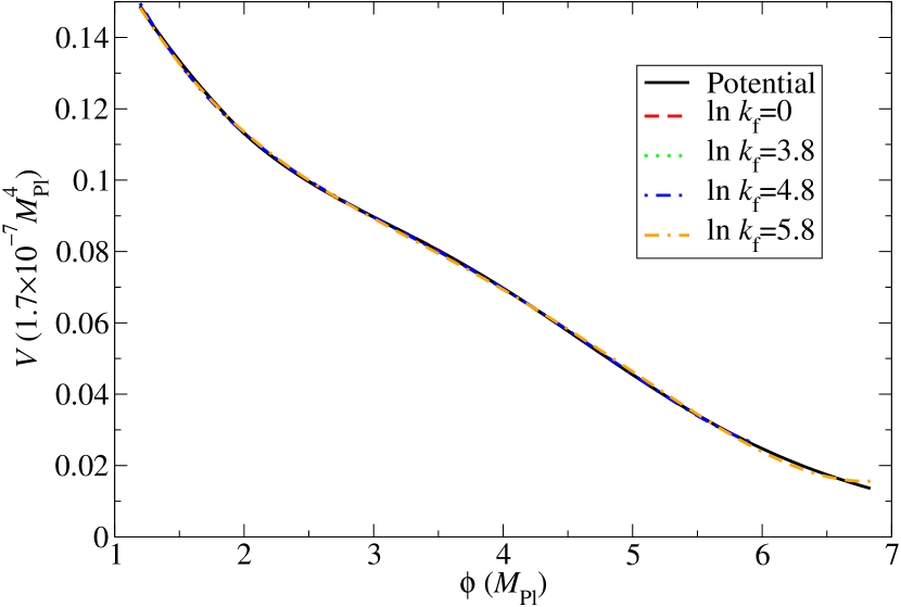
Figure 16: The reconstructed inflaton potential, and a series of renormalizable approximate potentials, which are matched to the exact result over increasingly large ranges of field values (indicated by the wave number of horizon crossing corresponding to the maximum field value in each range).

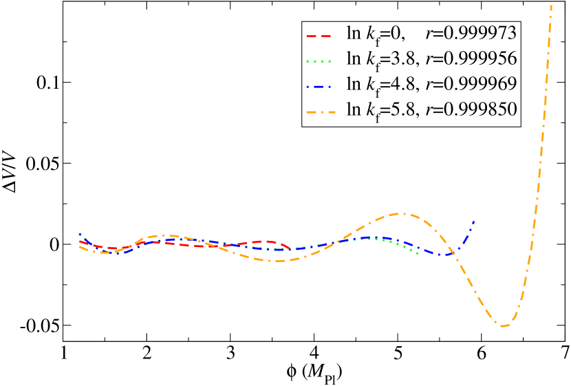
Figure 17: The fractional errors of the fitting potentials. The correlation coefficient $r$ for each fit is also shown next to the label ($r$ close to 1 corresponds to a good fit).

5 Conclusions

We have revisited the question of a running spectral index, motivated by the WMAP first year data. We are allowing for the possibility that the large running applies only in a limited region of $k$ space, where the CMB experiments are most sensitive and large scale structure is less sensitive. It is possible that even a parametrization with a running spectral index does not provide a good representation of the actual power spectrum over all observable scales. In fact we know that inflation cannot last for 60 e-foldings if running remains at the level of $dn/d\ln k=-0.1$—we find only $15-20$ e-foldings of exponential inflation—so it is also theoretically well-motivated to fit the spectrum separately in low and high regions of $k$ space. Something must change at larger $k$ just so that inflation can continue for another $40-45$ e-foldings.

Although the evidence for large running from the CMB is marginal, an improvement in $\chi^{2}$ of 3, requiring the addition of two (although somewhat degenerate) parameters, we have argued that it is based on more than just the first few multipoles of the temperature anisotropy; in fact, including the TE polarization data makes the first few multipoles unfavorable toward running. Rather, one observes a steady accumulation of $\Delta\chi^{2}$ as more low multipoles are dropped, with a sharp drop occuring in the region of $l$ near $40$. Even though this is still in the region where errors in the WMAP data are limited by cosmic variance, it will be interesting to see if there any significant changes when the next two years of data will be released.

Even though the large running scenario may be unlikely, it is interesting to pursue its consequences, given that it is not ruled out by the data. Since the slow-roll parameters do not remain very small over the entire inflationary trajectory, it may be useful to have a method of reconstruction of the inflaton potential which is not based on the slow-roll expansion around a particular pivot point, but instead satisfies the slow-roll prediction for the power spectrum (computed to any desired order in the slow-roll expansion) at every point in $\phi$ or $k$ space. We have devised an integration method of reconstructing $V(\phi)$ directly from $P(k)$, based on the Hamilton-Jacobi formalism, which has this property, and is also simple to implement numerically. We have shown how corrections to any order in the slow-roll expansion can be implemented without significantly complicating the algorithm. This method may be of interest in itself, independently of whether the running spectrum is confirmed by future data.

We demonstrated the reconstruction method by deriving the family of inflaton potentials that reproduce the best-fit large running spectrum. We subsequently focused on the unique potential which gives a large enough tensor-to-scalar ratio $r$ to be consistent with the best-fit spectrum. We pointed out that this is only possible when the running is cut off at low $k$ values; otherwise $r$ itself runs toward smaller values so quickly with $k$ that it falls below the desired value $r\cong 0.5$ before the pivot point $k_{0}$ is reached. This is a new observation, though anticipated by [10]. The large tensor contribution is one of the interesting features of the large running model; it puts the scale of inflation as high as possible (we find $V^{1/4}=3.5\times 10^{16}$ GeV) and it provides the greatest hope that direct evidence of tensor modes might be seen in the CMB. It also provides the best chance of uniquely fixing the inflaton potential, since without the tensor spectrum, and in the absence of a specific model, it is always possible to lower the scale of inflation while simultaneously making it flatter, to keep the scalar power fixed. We have shown that a renormalizable potential provides a good fit to the actual reconstructed potential over the limted region of field space where inflation occurs, even though the field values are Planckian. This provides another intriguing aspect to the large-running model: if true, it may give us an inflationary window on physics at the Planck scale.

Acknowledgments. We thank Gil Holder, Antony Lewis, Andrew Liddle, and Licia Verde for helpful information, discussions, or advice about CosmoMC. L. Hoi is supported by a postgraduate scholarship of the Tertiary Education Services Office, Macao SAR. We are also supported by NSERC of Canada and FQRNT of Québec.

References

- [1] C. L. Bennett et al., “First Year Wilkinson Microwave Anisotropy Probe (WMAP) Observations: Preliminary Maps and Basic Results,” Astrophys. J. Suppl. 148, 1 (2003) [arXiv:astro-ph/0302207].
- [2] H. V. Peiris et al., “First year Wilkinson Microwave Anisotropy Probe (WMAP) observations: Implications for inflation,” Astrophys. J. Suppl. 148, 213 (2003) [arXiv:astro-ph/0302225].
- [3] A. Kosowsky and M. S. Turner, “CBR anisotropy and the running of the scalar spectral index,” Phys. Rev. D 52, 1739 (1995) [arXiv:astro-ph/9504071].
- [4] S. Hannestad, S. H. Hansen and F. L. Villante, “Probing the power spectrum bend with recent CMB data,” Astropart. Phys. 16, 137 (2001) [arXiv:astro-ph/0012009].
- [5] S. Hannestad, S. H. Hansen, F. L. Villante and A. J. S. Hamilton, “Constraints on inflation from CMB and Lyman-alpha forest,” Astropart. Phys. 17, 375 (2002) [arXiv:astro-ph/0103047].
- [6] S. L. Bridle, A. M. Lewis, J. Weller and G. Efstathiou, “Reconstructing the primordial power spectrum,” Mon. Not. Roy. Astron. Soc. 342, L72 (2003) [arXiv:astro-ph/0302306].
- [7] M. Tegmark et al. [SDSS Collaboration], “Cosmological parameters from SDSS and WMAP,” Phys. Rev. D 69, 103501 (2004) [arXiv:astro-ph/0310723].
- [8] D. J. H. Chung, G. Shiu and M. Trodden, “Running of the scalar spectral index from inflationary models,” Phys. Rev. D 68, 063501 (2003) [arXiv:astro-ph/0305193].
- [9] J. E. Lidsey, A. R. Liddle, E. W. Kolb, E. J. Copeland, T. Barreiro, and M. Abney, “Reconstructing the Inflaton Potential – an Overview,” Rev. Mod. Phys. 69, 373 (1997) [arXiv:astro-ph/9508078].
- [10] D. J. H. Chung and A. Enea Romano, “Approximate consistency condition from running spectral index in slow-roll inflationary models,” arXiv:astro-ph/0508411.
- [11] M. Cortes and A. R. Liddle, “The Consistency Equation Hierarchy in Single-Field Inflation Models,” Phys. Rev. D 73, 083523 (2006) [arXiv:astro-ph/0603016].
- [12] R. Easther, “Folded inflation, primordial tensors, and the running of the scalar spectral index,” arXiv:hep-th/0407042.
- [13] M. Kawasaki, M. Yamaguchi and J. Yokoyama, “Inflation with a running spectral index in supergravity,” Phys. Rev. D 68, 023508 (2003) [arXiv:hep-ph/0304161]. M. Yamaguchi and J. Yokoyama, “Chaotic hybrid new inflation in supergravity with a running spectral index,” Phys. Rev. D 68 123520 (2003) [arXiv:hep-ph/0307373]. M. Yamaguchi and J. Yokoyama, “Smooth hybrid inflation in supergravity with a running spectral index and early star formation,” Phys. Rev. D 70, 023513 (2004) [arXiv:hep-ph/0402282].
- [14] G. Ballesteros, J. A. Casas and J. R. Espinosa, “Running spectral index as a probe of physics at high scales,” arXiv:hep-ph/0601134.
- [15] R. Brandenberger and P. M. Ho, “Noncommutative spacetime, stringy spacetime uncertainty principle, and density fluctuations,” Phys. Rev. D 66, 023517 (2002) [AAPPS Bull. 12N1, 10 (2002)] [arXiv:hep-th/0203119].
- [16] Q.-G. Huang and M. Li, “Running spectral index in noncommutative inflation and WMAP three year results,” arXiv:astro-ph/0603782; “CMB Power Spectrum from Noncommutative Spacetime,” JHEP 0306, 014 (2003) [arXiv:hep-th/0304203]; “Noncommutative Inflation and the CMB Multipoles,” JCAP 0311, 001 (2003) [arXiv:astro-ph/0308458]; “Power Spectra in Spacetime Noncommutative Inflation,” Nucl. Phys. B 713, 219 (2005) [arXiv:astro-ph/0311378].
- [17] A. Ashoorioon, J. L. Hovdebo and R. B. Mann, “Running of the spectral index and violation of the consistency relation between tensor and scalar spectra from trans-Planckian physics,” Nucl. Phys. B 727, 63 (2005) [arXiv:gr-qc/0504135].
- [18] J. M. Cline and H. Stoica, “Multibrane inflation and dynamical flattening of the inflaton potential,” Phys. Rev. D 72, 126004 (2005) [arXiv:hep-th/0508029].
- [19] U. Seljak et al., “Cosmological parameter analysis including SDSS Ly forest and galaxy bias: Constraints on the primordial spectrum of fluctuations, neutrino mass, and dark energy,” Phys. Rev. D 71, 103515 (2005) [arXiv:astro-ph/0407372].
- [20] L. A. Popa, C. Burigana and N. Mandolesi, “Non-linear evolution of the cosmological background density field as diagnostic of the cosmological reionization,” New Astron. 9, 189 (2004) [arXiv:astro-ph/0309785].
- [21] H. M. Hodges and G. R. Blumenthal, “Arbitrariness of Inflationary Fluctuation Spectra,” Phys. Rev. D 42 3329 (1990).
- [22] M. Joy and E. D. Stewart, “From the spectrum to inflation: A second order inverse formula for the general slow-roll spectrum,” JCAP 0602, 005 (2006) [arXiv:astro-ph/0511476]; “Reconstruction of the inflationary parameters from the second order general slow-roll spectrum,” AIP Conf. Proc. 805, 455 (2006). K. Kadota, S. Dodelson, W. Hu and E. D. Stewart, “Precision of inflaton potential reconstruction from CMB using the general slow-roll approximation,” Phys. Rev. D 72, 023510 (2005) [arXiv:astro-ph/0505158]. R. Easther and W. H. Kinney, “Monte Carlo reconstruction of the inflationary potential,” Phys. Rev. D 67, 043511 (2003) [arXiv:astro-ph/0210345]. I. J. Grivell and A. R. Liddle, “Inflaton potential reconstruction without slow-roll,” Phys. Rev. D 61, 081301 (2000) [arXiv:astro-ph/9906327]. E. J. Copeland, I. J. Grivell, E. W. Kolb and A. R. Liddle, “On the reliability of inflaton potential reconstruction,” Phys. Rev. D 58, 043002 (1998) [arXiv:astro-ph/9802209]. M. S. Turner and M. J. White, “Dependence of Inflationary Reconstruction upon Cosmological Parameters,” Phys. Rev. D 53, 6822 (1996) [arXiv:astro-ph/9512155]. A. R. Liddle and M. S. Turner, “Second order reconstruction of the inflationary potential,” Phys. Rev. D 50, 758 (1994) [Erratum-ibid. D 54, 2980 (1996)] [arXiv:astro-ph/9402021]. E. J. Copeland, E. W. Kolb, A. R. Liddle and J. E. Lidsey, “Reconstructing the inflaton potential: Perturbative reconstruction to second order,” Phys. Rev. D 49, 1840 (1994) [arXiv:astro-ph/9308044].
- [23] A. G. Muslimov, “On the scalar field dynamics in a spatially flat Friedman universe,” Class. Quantum Grav. 7, 231 (1990).
- [24] D. S. Salopek and J. R. Bond, “Nonlinear evolution of long-wavelength metric fluctuations in inflationary models,” Phys. Rev. D 42, 3936 (1990).
- [25] A. Lewis and S. Bridle, “Cosmological parameters from CMB and other data: a Monte-Carlo approach,” Phys. Rev. D 66, 103511 (2002) [arXiv:astro-ph/0205436].
- [26] W. L. Freedman et. al., “Final Results from the Hubble Space Telescope Key Project to Measure the Hubble Constant,” Astrophys. J. 553, 47 (2001) [arXiv:astro-ph/0012376].
- [27] C. L. Kuo et al., “High Resolution Observations of the CMB Power Spectrum with ACBAR,” Astrophys. J. 600, 32 (2004) [arXiv:astro-ph/0212289].
- [28] C. Dickinson et al., “High sensitivity measurements of the CMB power spectrum with the extended Very Small Array,” Mon. Not. R. Astron. Soc. 353, 732 (2004) [arXiv:astro-ph/0402498].
- [29] A. C. S. Readhead et al., “Extended Mosaic Observations with the Cosmic Background Imager,” Astrophys. J. 609, 498 (2004) [arXiv:astro-ph/0402359].
- [30] W. J. Percival et al., “Parameter constraints for flat cosmologies from CMB and 2dFGRS power spectra,” Mon. Not. R. Astron. Soc. 337, 1068 (2002) [arXiv:astro-ph/0206256].
- [31] A. R. Liddle, “How many cosmological parameters?,” Mon. Not. Roy. Astron. Soc. 351, L49 (2004) [arXiv:astro-ph/0401198].
- [32] L. Hoi and J. M. Cline, “Inflationary Spectral Indices and Potential Reconstruction,” in preparation (2006).
- [33] A. Makarov, “On the Accuracy of Slow-Roll Inflation Given Current Observational Constraints,” Phys. Rev. D 72 083517 (2005) [arXiv:astro-ph/0506326].
- [34] E. D. Stewart and D. H. Lyth, “A More accurate analytic calculation of the spectrum of cosmological perturbations produced during inflation,” Phys. Lett. B 302, 171 (1993) [arXiv:gr-qc/9302019].