Restoring Color-magnitude Diagrams with the Richardson-Lucy Algorithm

We present an application of the Richardson-Lucy algorithm to the analysis of color-magnitude diagrams by converting the CMD into an image and using a restoring point spread function function (psf) derived from the known, often complex, sources of error. We show numerical experiments that demonstrate good recovery of the original image and establish convergence rates for ideal cases with single gaussian uncertainties and poisson noise using a $\chi^{2}$ statistic. About 30-50 iterations suffice. As an application, we show the results for a particular case, the Hipparcos sample of the solar neighborhood where the uncertainties are mainly due to parallax which we model with a composite weighted gaussian using the observed error distributions. The resulting psf has a slightly narrower core and broader wings than a single gaussian. The reddening and photometric errors are considerably reduced by restricting the sample to within 80 pc and to $M_{V}\leq 3.5$. We find that the recovered image, which has a narrower, better defined main sequence and a more clearly defined red giant clump, can be used as input to stellar evolution modeling of the star formation rate in the solar vicinity and, with more contributing uncertainties taken into account, for general Galactic and extragalactic structure and population studies.

1 Introduction

The color-magnitude diagram (CMD) is the key tool for studying evolution in stellar populations. However, when interpreting cluster and field CMDs we have to face different problems. For clusters, unless they are very nearby and large, the stars can be assumed to be at nearly the same distance and therefore even if the absolute luminosities are unknown their relative values are well determined. Unless the system is very young, of order the pre-main sequence contraction time, the stars can be assumed to have the same age and metallicity since their formation occurs essentially instantaneously. The uncertainties are, consequently, mainly photometric and also due to interstellar reddening (but this, like the distance, can initially be assumed identical for all members) or in crowded fields due to confusion. In contrast, for field stars, the uncertainties affecting the CMD are mainly due to parallax errors and reddening, which are different for each star, so the relative as well as absolute luminosities are inherently uncertain. Since the aim of field studies is to determine the structure and the star formation and metallicity histories of the solar neighborhood, any sample must be assumed to have formed over a long time. To unravel these histories requires a different approach than usually adopted for the treatment of the aggregate CMD. Our aim in this study is to show how to obtain a cleaned input for such analyses that is, in effect, a restoration of the intrinsic distribution to the limit of the errors. A CMD may be regarded as an image, the ’intensity’ being the number of stars in a bin of some photometric indices or effective temperature and luminosity, affected by a point spread function (psf) that originates from the error distributions of the parallaxes, interstellar reddening, and photometry and we propose using the same techniques that have been developed for image restoration.

Specifically, we apply the Bayesian Richardson-Lucy algorithm (Richardson richardson (1972), Lucy lucy74 (1974)) to an observed CMD. This method is very well known in the astronomical community and has been broadly applied to recover data from images and histograms (see, e.g. Bertero & Boccacci BB (2005) and references therein). Here we suggest another use, this time for the study of stellar populations. If we grid a CMD by building a two dimensional histogram in, say, $M_{V}$ and $B-V$, the data is an image blurred by a psf that is the matrix produced by the observational errors. The analysis then becomes a deconvolution problem. From this point of view, the loss of information about single stars is compensated by the opportunity to analyze the sample data in a statistically consistent sense using imaging methods. Our intent is to recover, as closely as possible within the limits of the psf, the intrinsic CMD for comparison with stellar isochrones that may then be analyzed by any of many available statistical methods (see especially Tolstoy & Saha tol (1996), Hernandez et al. her99 (1999),her00 (2000)). Although in what follows we use the Hipparcos solar neighborhood sample for illustration, the technique is as general as the RL algorithm itself and we emphasize that our aim is to propose a new view of how to treat observatioanl CMD data for stellar and galactic evolution.

2 Use of the algorithm

Bayes’ theorem provides the relationship between the probability of a hypothesis (model parameters) conditional on a given data, $P(M|D)$ (posterior), and the probability of the data conditional on the hypothesis, $P(D|M)$, and the prior probability $P(M)$:

$$P(M|D)=\frac{P(D|M)P(M)}{\int P(D|M)P(M)}$$ (1)

where $M$ are the values for the parameters of the model (the hypothesis) and $D$ are the measured data. The prior is the probability of any hypothesis being true before empirical data, the posterior probability is what we can know about hypothesis after the observation (how likely, given the observations, our model is as an explanation of the data); $P(D|M)$, the likelihood, is the chance of the observation $D_{n}$ given the model $M_{n}$ for some sample $n$ (e.g. Jaynes 2003). First, assuming the intrinsic noise in the data is poisson distributed, the conditional probability is given by:

$$P(D|M)=\prod^{N}_{n=0}\frac{\exp{(-{M}_{n}){{M}_{n}}^{D_{n}}}}{{D_{n}}!}$$ (2)

where the product is taken over N bins. The intrinsic fluctuations are poisson distributed.

The psf is from the photometric and parallax errors. The data value is the number of stars in the $nth$ bin which result from sampling some initial mass function (IMF) $\phi(m)$ at a star formation rate (SFR), $\psi(t)$, and depending on some metallicity history, $Z(t)$; if we fix $\phi$ the other two are the functions should be recoverable from the sample. The relevance to CMDs is that, depending on the type of data, there may be several contributing factors to the total psf, $K$ e.g. errors in photometry, parallaxes, and proper motions, and uncertainties in reddening, unresolved binary companions, etc.. The combination of blurring and fluctuations on the final image is:

$$({\rm image})=K\star({\rm object})+{\cal N}$$ (3)

where ${\cal N}$ is the noise. Richardson (richardson (1972)) and Lucy (lucy74 (1974)) were the first to propose an iterative inversion algorithm (hereinafter R-L algorithm) for deconvolution:

$$f^{(k+1)}=f^{(k)}\,K\star\left(\frac{D}{K\star f^{(k)}}\right)$$ (4)

with $f^{(k)}$ is the object estimation after the k-th iteration and $D$ is the data. The method is derived assuming poisson noise and taking a constant prior information $P(M)$ in equation 1 (non-informative prior). It can be shown that the algorithm converges to a restoration that when re-blurred by the psf is close to the data in a maximum likelihood sense (for details see e.g. Shepp & Vardi shepp (1982)).

Although the Hipparcos data is the subject of our application of the R-L algorithm, its possible use extends to any binned CMD. Since the specific deconvolution problem must be preceded by a careful analysis of the associated uncertainties, the following section discusses the sources of blur in the Hipparcos data. In the following sections we show tests based on convolving synthetic CMDs, mimicking the solar neighborhood Hipparcos sample, with different psfs and performed restorations using the R-L method. We show examples of experiments that demonstrate successful image restoration under various assumed point spread functions. The same analysis was performed after adding poisson noise and using the $\chi^{2}$ statistic as the convergence parameter. The last section shows the result of applying the method to the real data using an observationally derived psf and discuss some applications.

3 Hipparcos uncertainties

Our sample was selected using two criteria. The stars are all brighter than $V\sim 8$, which is comfortably within the completeness interval assumed by the Hipparcos collaboration of between 7.3 and 9 mag depending on Galactic latitude and color (e.g. Perryman et al. 1995), and are within 80 pc from the Sun, corresponding to an absolute magnitude of $3.5$ mag at our adopted limit. The parallax precision is generally better than 10% and the nonlinearity bias is assumed very small (e.g. Arenou & Luri arenou2 (1999)). The histogram of the absolute visual magnitude error distribution for our sample, obtained by propagating the parallax errors, (see fig. 1), shows a mean error of about 0.10 mag with a standard deviation of about 0.05 mag. The same figure shows the absolute magnitude error distribution for stars in three bins of absolute visual magnitude, respectively $2-2.5,2.5-3,3-3.5\,\,\mathrm{mag}$. The histograms for stars with $2<M_{V}<2.5$ and $2.5<M_{V}<3$ are the same within the poisson fluctuations, while the histogram $3-3.5$ presents a slightly systematic shift (about $0.01-0.02$ mag) toward bigger errors. This last feature may be due to the selection in absolute magnitude. Moreover, the parallax precision decreases with distance so the larger absolute magnitude errors found in the $3-3.5$ mag could be explained by a greater mean distance of the sample. It is, however, a small effect so the distribution for the absolute magnitude error, to fair accuracy, was assumed to be independent of the position in the CMD as a first assumption about the psf.

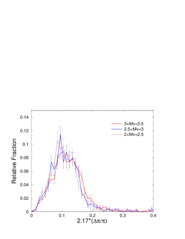
Figure 1: The absolute magnitude error distribution for Hipparcos stars brighter than $M_{V}=3.5$ and nearer than 80 pc for different intervals of absolute magnitude. The error bar is poissonian. The figure shows the general agreement among the curves.

The photometric error for stars brighter than $M_{V}=3.5$ is generally $<0.02$ mag but there is also an high error tail due to giant and clump stars. These last groups comprise only $1-2\%$ of the total sample and since the color uncertainty is so small, compared to the absolute magnitude error, we here assume that it can be neglected. The method we’ll present can, however, be easily generalized to two dimensions (for instance in treating crowding and other photometric errors in observations of fields in resolved galaxies).

4 Tests with artificial data

Before using our method to real data, we have to test its ability in restoring CMDs on the basis of artificial data. We begin by modeling the psf with a gaussian. Considering the relative uncertainties in color and absolute magnitude we chose $\sigma=0.1\,\mathrm{mag}$, the mean value found in the observational distribution. The error on $B-V$ is negligible so the convolution and deconvolution affect only the absolute magnitudes but the method can be generalized to two dimensions. The synthetic CMD (fig. 2-a) was generated with a Monte Carlo technique (see for details Castellani et al. cast (2002) and Cignoni et al. cign (2003)) using a power law with a Salpeter exponent (see Kroupa krou (2001)), a flat SFR ($\psi={\rm constant}$) and an observational age-metallicity relation $Z(t)$ from Nördstrom et al. nord (2004). The artificial stars were placed on grid of tracks (Pisa Evolutionary Library). No binaries have been included but this is not an inherent limitation if appropriate estimates are available for their contributions (e.g. Hurley & Tout hur (1998)). The synthetic CMD contains approximately the same number of stars brighter than $M_{V}=3.5$ of the selected Hipparcos CMD, so we can avoid possible differences due to the statistical fluctuations. Figure 2-a shows the synthetic CMD and Fig. 2-b shows the pixelated version, binned with a step size of $0.05$ mag in both coordinates so the psf has a $\sigma$ of 2 pixels. This choice of the bin size is a practical compromise: smaller values produce statistical fluctuations too large which could be a problem because noise amplification is a real drawback with iterative algorithms. Larger bins reduce or eliminate the effectiveness of the restoration, reducing also the potential information content of the dataset. In our case, the observational uncertainty in $B-V$ is negligible compared to the mean error in the absolute magnitude so we did not test the effects of blurring in color and do not need any finer binning. Choosing 0.05 mag for the bin size minimized the problems mentioned above.

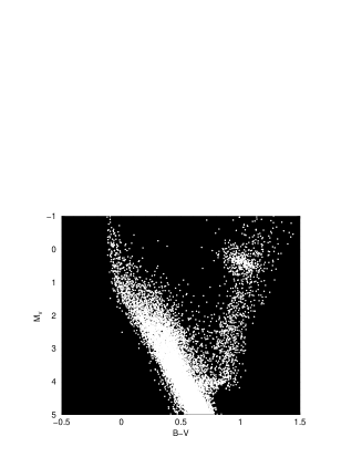
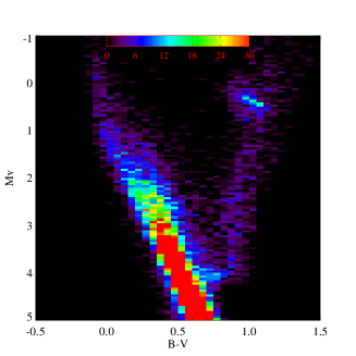
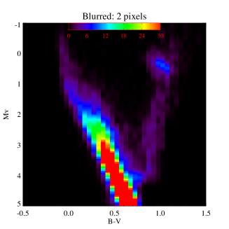
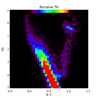
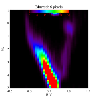
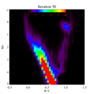
Figure 2: Synthetic tests demonstrating the recovery achieved using the R-L algorithm. From top left: (a) Synthetic CMD, (b) 2-D histogram for the synthetic CMD; (c) blurred with 2 pixels gaussian psf; (d) restored image after 50 iterations. For contrast, (e) synthetic image blurred with 6 pixels gaussian; (f) restored image for 6 pixels blurring after 50 iterations (see text for details).

Convolving the synthetic CMD with a gaussian ($\sigma=2$ pixels) produces the image shown in figure 2-c. The result after 50 iterations is shown in figure 2-d. The restored image is quite close to the original. To quantify this match we needed a convergence criterion (a rule that stops the algorithm when further iterations do not significantly improve the result). Since the original papers it has been convenient to take $\chi^{2}$ as this control parameter (see Richardson richardson (1972), Lucy lucy74 (1974), Bi & Börner bi (1994), Molina et al. molina (2001)):

$$\chi_{k}^{2}=\frac{(\overline{g}-g^{k})^{2}}{g^{k}}$$ (5)

where $\overline{g}$ is the blurred image and $g^{k}$ is the estimate of the observed image resulting after the $k$th iteration. Calculating the $\chi_{k}^{2}$ for each iteration we found a monotonically decreasing trend with an asymptotic value close to zero. This is because the synthetic CMD has been convolved with a psf without additional noise so R-L algorithm can perfectly recover the original CMD. To gain a better understanding of how the algorithm converges, we tried a broader psf with $\sigma=6$ pixels. The blurred image and the restoration results are shown in figures 2-e-f.

Thus far we have treated the case of ideal data (i.e. without noise). However, an important point when trying to recover the underlying image from noisy data is the sensitivity of the restoration algorithm to noise and its tendency to produce artifacts with successive iterations. The problem is that any convolution is a smoothing operation and, in the Fourier domain, this reduces the high spatial frequencies that characterizes the small scales of the image. Methods like the R-L algorithm attempt to remove the smoothing, but this is not straightforward since noise is also present. As originally suggested by Lucy (lucy74 (1974)), the estimate $f^{k}$ of the real distribution does not converge as $f^{k+1}-f^{k}\rightarrow 0$ as $k\rightarrow\infty$; in fact, after a best estimate of $f^{\tilde{k}}$ the agreement get worse and artifacts may appear because of small scale fluctuations. Since the R-L algorithm is not regularized, when the iteration number increases noise amplifies in the solution. In practice, the iteration number must be limited to find an acceptable compromise between resolution and stability. To test how the statistical uncertainties present in the data can influence the deconvolved image, we blurred a CMD with a psf with a $\sigma=2$ pixels and added poisson noise (see figure 3-a). The restored CMD after 50 iterations is shown in figure 3-b.

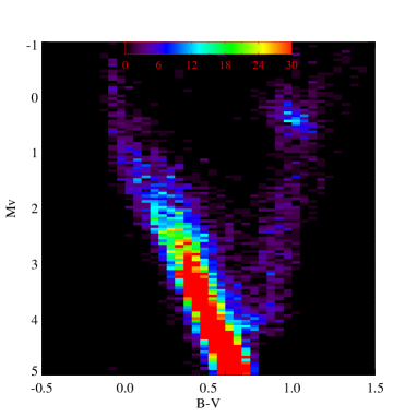
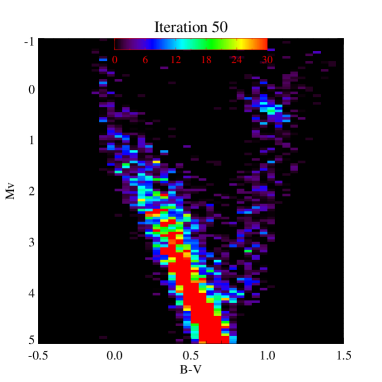
Figure 3: (a) 2 pixels blurring plus poisson noise; (b) restored CMD after 50 iterations.

As expected, the result is very different from the case from the previous case: the addition of poisson noise prevents the recovery of the exact morphology of the original CMD. In fact, with continued iterations the CMD becomes grainier. The result is better for the most populated regions of the CMD, those with high signal to noise ratio, where the CMD features are not buried by noise. We find that the $\chi^{2}$, after $\sim 50-100$ iterations, reaches a plateau (see figure 4) and stabilizes around this value. This actually illustrates the utility of the image approach since such changes can be easily modeled in a controlled way and the changes can be statistically monitored in a way that bootstrapping, for instance, cannot show.

Figure 4: $\chi^{2}$ versus iterations number (case with blurring and noise).

In order to preserve the CMD morphology, since the algorithm improves the statistical properties of the sample but destroys local information, the iterations are stopped after about 50 cycles when the bulk of the restoration has been achieved.

5 Application to real data

Passing to real data, the first problem is to account for the distribution of parallax errors. In principle, we cannot adopt a mean error value as we did in the previous simulations ($\sigma=2$ pixels). If we do not take this point into account and blindly apply the algorithm with a $\sigma=2$ pixels wide gaussian, the restorations give the $\chi^{2}$ values shown in figure 5 (star symbol).

Figure 5: $\chi^{2}$ versus iteration number for the restoration with gaussian psf (star) and pseudo-gaussian psf (filled circles).

A more realistic approach is to use the full information contained in the data error distribution by forming a psf from a linear combination of gaussians using the data shown in Fig. 1:

$$K=\frac{1}{A}\sum_{i}\frac{1}{H_{i}}\,\frac{1}{\sigma_{i}\sqrt{2\pi}}\exp\left(\frac{-x^{2}}{2\sigma_{i}^{2}}\right)$$ (6)

where the $A$ factor is a normalization constant, the weights $H_{i}$ are the histogram values from figure 1, i.e. the fraction of stars with absolute magnitude error between $(\Delta M_{V})_{i}$ and $(\Delta M_{V})_{i}+\delta$), and the $\sigma_{i}$ are the values $(\Delta M_{V})_{i}$ . The resulting psf (see figure 6) is nearly symmetric with a narrower core and broader wings than a gaussian with the same full width, and with the dispersion given by $\sigma=\sum_{j}\sigma_{j}/H_{j}$, the weighted histogram.

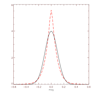
Figure 6: The solid line is a gaussian function with $\sigma=2$ pixels. The dashed line represents the function obtained from a linear combination of gaussians with standard deviations and weights given by data.

We obtain the sequence of restorations shown in figure 7 using this composite psf. Now the $\chi^{2}$ converges faster (see the curve with filled circles in figure 5) to smaller values so the iterations can be stopped sooner. The main results of the restoration process is to compact the CMD features along the deconvolution axis (absolute magnitude axis). We find that (a) the red clump region is compressed and new features appear, (b) the giant and sub-giant regions are both better defined, and (c) the main sequence blue edge is now sharper. These improvements in the CMD may appear small, but the restored CMD is the cleanest restored data we expect to find that is consistent with the uncertainties in a Bayesian sense.

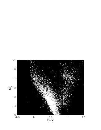
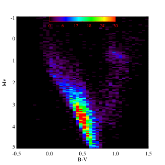
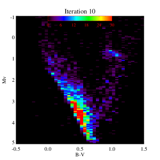
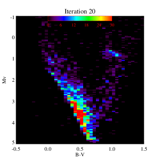
Figure 7: (a) Hipparcos CMD. (b) 2-D histogram for the Hipparcos CMD. (c)-(d) Restorations with the pseudo-gaussian psf (the number of iteration is labeled).

6 Conclusions

The aim of this study has been to demonstrate a method for recovering as much information as possible from binned color-magnitude diagrams that can then serve as input for evolutionary studies of stellar ensambles. The resulting reconstructions should be the best cleaned data set with which to perform analyses of the star formation rates and metallicity evolution over time for complex samples. The advantage of this approach over bootstrapping comes from the ease of including in the likelihood function a broad range of processes (known or hypothetical) that affect the location of stars within the observed CMD. Although we have concentrated here on a particular algorithm, the Richardson-Lucy method, there is in principle no restriction and others, e.g. maximum entropy, could be used instead. A study of the star formation history of the solar neighborhood will be the topic of a future paper (Cignoni et al. 2006, in preparation).

- (1) Arenou F. & Luri X., 1999, Distances and absolute magnitudes from trigonometric parallaxes, ASP Conference Series 167, D. Egret and A. Heck, p. 13
- (2) Bertero, M. & Boccacci, P. 2005, A&A, 437, 369
- (3) Bi, H. & Börner, G. 1994, A&AS, 108, 409
- (4) Castellani, V., Cignoni, M., Degl’Innocenti, S., Petroni, S., & Prada Moroni P. G. 2002, MNRAS, 334, 69
- (5) Cignoni, M., Ph.D. thesis, Dept. of Physics, University of Pisa
- (6) Cignoni, M., Prada Moroni, P. G., & Degl’Innocenti, S. 2003, MemSAIt, 3, 143
- (7) Hernandez, X., Valls-Gabaud, D., & Gilmore, G., 1999, MNRAS, 304, 705
- (8) Hernandez, X., Valls-Gabaud, D., & Gilmore, G. 2000, MNRAS, 316, 605
- (9) Hurley, J. & Tout, C. A. 1998, MNRAS, 300, 977
- (10) Jaynes, E.T., 2003, Probability Theory: The Logic of Science Cambridge: Cambridge Univ. Press
- (11) Kroupa, P. 2001, MNRAS, 322, 231
- (12) Lucy, L. B. 1974, AJ 79, 745
- (13) Molina, R., Núñez, J., Cortijo, F. J., Mateos, J. 2001, IEEE Signal Processing Magazine, 18(2), 11-29
- (14) Nördstrom, B., Mayor, M., Andersen J., Holmberg, J., Pont, F., Jorgensen, B. R., Olsen, E. H., Udry, S., & Mowlavi, N. 2004, A&A, 418, 989
- (15) Perryman, M. A. C. et al. 1995, A&A, 304, 69
- (16) Richardson, W. H. 1972, JOSA., 62, 55
- (17) Shepp, L. A. & Vardi, Y. 1982, IEEE Trans. Medical Imaging, MI-1, 113
- (18) Tolstoy, E., & Saha, A., 1996, ApJ, 462, 672