High resolution X-ray spectroscopy of bright O type stars

Abstract

Archival X-ray spectra of the four prominent single, non-magnetic O stars $\zeta\,$Pup, $\zeta\,$Ori, $\xi\,$Per, $\zeta\,$Oph, obtained in high resolution with Chandra hetgs/meg have been studied. The resolved X-ray emission line profiles provide information about the shocked, hot gas which emits the X-radiation, and about the bulk of comparably cool stellar wind material which partly absorbs this radiation. In the present paper we synthesize X-ray line profiles with a model of a clumpy stellar wind. We find that the geometrical shape of the wind inhomogeneities is important: better agreement with the observations can be achieved with radially compressed clumps than with spherical clumps. The parameters of the model, i.e. chemical abundances, stellar radius, mass-loss rate and terminal wind velocity, are taken from existing analyses of UV and optical spectra of the program stars. On this basis we also calculate the continuum absorption coefficient of the cool-wind material, using the Potsdam Wolf-Rayet (PoWR) model atmosphere code. The radial location of X-ray emitting gas is restricted from analyzing the fir line ratios of helium-like ions. The only remaining free parameter of our model is the typical distance between the clumps; here we assume that at any point in the wind there is one clump passing by per one dynamical timescale of the wind. The total emission in a model line is scaled to the observation. There is a good agreement between synthetic and observed line profiles. We conclude that the X-ray emission line profiles in O stars can be explained by hot plasma embedded in a cool wind which is highly clumped in the form of radially compressed shell fragments.

1 Introduction

Young and massive O-type stars possess strong stellar winds. The winds are fast, with typical velocities up to 2500 km/s, and dense, with mass-loss rates $\dot{M}\raisebox{-1.72218pt}{$\stackrel{{\scriptstyle>}}{{\scriptstyle\sim}}$}10^{-7}M_{\odot}/{\rm yr}$. The driving mechanism for the mass-loss from OB stars has been identified with radiation pressure on spectral lines (Castor, Abbot & Klein, 1975). However, it was pointed out early (Lucy & Solomon, 1970) and later further investigated (Owocki & Rybicki, 1984) that the stationary solution for a line-driven wind is unstable; small perturbation grow quickly and result in strong shocks giving rise to the production of hot gas and emitting of X-rays.

X-rays from hot OB type stars were discovered by the Einstein X-ray observatory (Harnden et al., 1979; Seward et al., 1979). A large number of OB type stars was detected by the Rosat All Sky Survey (Berghöfer, Schmitt & Cassinelli 1996), providing firm evidence that the X-ray emission is intrinsic for O star winds. The low resolution Rosat spectrum of the O-type supergiant $\zeta\,$Pup was modeled by Hillier et al. (1993). In order to explain the apparent weakness of absorption in the spectrum, Hillier et al. (1993) postulated that the X-rays are emitted far out in the stellar wind, at distances larger that $100\,R_{*}$, by an optically thin shell expanding at constant velocity. The emission from such shell would produce a broad rectangular box-like line.

A box-like line profile is distinctly different from a skewed triangular line expected from radiation arising in the wind acceleration zone and attenuated in the wind (MacFarlane et al., 1991). Ignace (2001) demonstrated that the asymmetry of the line correlates with the wind opacity and density. In a more optically thick wind the lines are more blue-shifted. Since atomic opacity is wavelength dependent, the lines are expected to differ in shape across the spectrum, with larger blue-shift at wavelengths where the wind opacity is higher.

X-ray generation in the wind acceleration zone is predicted in the model by Feldmeier, Puls & Pauldrach (1997), who showed from hydrodynamic simulations that dense cool shells of gas form in deep wind regions. Collisions of these shells can lead to strong shocks. X-rays originate from radiatively cooling zones behind the shock fronts. The hot X-ray emitting plasma is thermal, has a small filling factor, and is optically thin. The produced X-rays can be significantly attenuated by the overlying cool stellar wind. Hence the blue-shifted lines are expected.

High-resolution X-ray spectra of O-type stars were obtained for the first time by the Chandra X-ray observatory (Waldron & Cassinelli, 2001). The resolved emission line profiles offered a stringent test for the theory. The analysis of the line ratios from He-like ions in $\zeta\,$Ori and $\zeta\,$Pup  constrained the regions of X-ray formation relatively close to the stellar surface. The line width was measured to be less than corresponding to the maximum velocity, confirming that the line emission originates in the wind acceleration zone. Line blue-shifts were also detected, indicating wind attenuation (Cassinelli et al., 2001).

However, the data revealed that the line blue-shifts do not change significantly for lines at different wavelengths in contrast to what was expected (Waldron & Cassinelli, 2001; Cassinelli et al., 2001). Moreover, the line fitting using the ”standard model” of smooth homogeneous wind was not able to to reproduce the lines observed in non-magnetic single O stars unless with significantly reduced mass-loss rates (Kramer, Cohen & Owocki 2003, Cohen et al., 2006).

There is a good reason to believe that mass-loss rates from O stars are need to be revised downwards. A plenitude of observational and theoretical evidence indicates the clumped inhomogeneous nature of O star winds (Repolust et al., 2004, Bouret, Lanz & Hillier 2005, Fullerton, Massa & Prinja 2006). The empirical mass-loss rates of WR stars are generally reduced by factors of a few in a clumped wind (Hamann & Koesterke, 1998), but it is still not known by how much exactly in case of O stars (Puls et al., 2006).

Radiative transfer in a stochastic medium is distinctly different from the transfer in a smooth medium (Pomraning, 1991), especially when the clumps are not necessarily optically thin. Therefore, it is inconsistent to apply the smooth-wind formalism in order to model spectral lines in a wind where the mass-loss rate estimates are based on the assumption of wind clumping.

The transport of X-rays in a clumped stellar wind was studied analytically and numerically by Feldmeier, Oskinova & Hamann (2003) and Oskinova, Feldmeier & Hamann (2004), respectively. Motivated by the prediction of hydrodynamic simulations that the cool-wind clumps are radially compressed, we considered the case of anisotropic wind opacity, where the optical thickness of a clump depends on its orientation. Feldmeier et al. (2003) showed and explained that the assumption of flattened wind clumps leads to nearly symmetric and blueshifted line shapes. A corresponding 2D stochastic wind model developed in Oskinova et al. (2004) demonstrated that clumping effectively reduces the wind opacity and its wavelength dependence. The latter effect leads to a similarity of the shapes of all X-ray lines. Recently, Owocki & Cohen (2006) used a similar model, but restricted to the specific case of isotropic clumps. In the latter model a symmetric line profile results only when the mean separation between optically thick clumps is quite large, of the order of a few stellar radii.

The main objective of the present paper is to compare, for the first time, the model lines from clumped winds with the lines observed in the X-ray spectra of the prominent single non-magnetic O stars $\zeta\,$Pup, $\xi\,$Per, $\zeta\,$Ori, and $\zeta\,$Oph.

Our basic strategy is to adopt the best available parameters for the stars and their winds, compute on their basis the model line profiles, and compare them with the observation. Thus we do not infer the model parameters from the line fitting, but instead answer the question whether the observed lines can be described in the framework of the X-ray transport in stochastic media.

We utilize the most recent empirical mass-loss rates of our sample stars, and evaluate the mass-absorption coefficient in the wind using state-of-the-art non-LTE atmosphere code. Observed X-ray spectra are analyzed to infer the zone of X-ray emission and the wind velocity field. The only remaining free parameter of our model is the average time interval between subsequent clumps passing the same point in the stellar wind. For this parameter we adopt the wind flow time, $R_{*}/\mbox{$v_{\infty}$}$.

With all model parameters defined, we model each line and compare it with the observation.

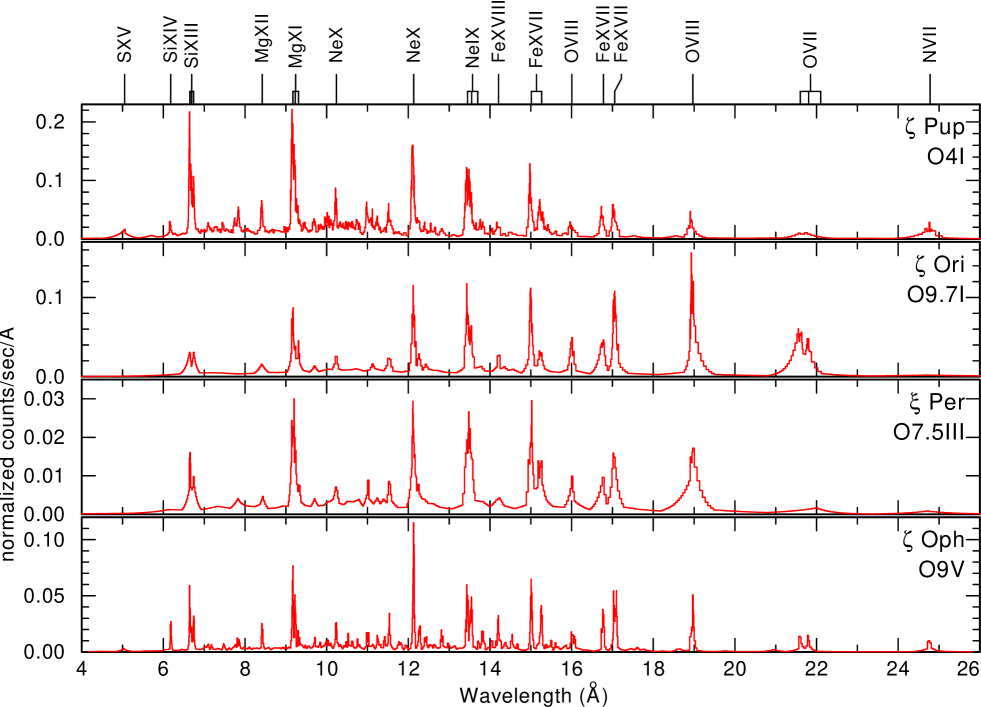
Figure 1: De-reddened hetgs/meg$\pm 1$ spectra of prominent O stars.

The paper is organized as follows. Observational evidences of strong wind clumping are discussed in Section 2. The observations and broad-band spectral properties of our sample stars are presented in Section 3. The analysis of line ratios of He-like ions, conducted in order to estimate the location and temperature of the X-ray emitting plasma, is presented in Section 4. Section 5 describes the stellar atmosphere model, and Section 6 briefly summarizes our radiative transfer technique for X-rays in a clumped stellar wind. The comparison of modeled and observed line profiles is done in Section 7, and a discussion follows in Section 8. Conclusions are presented in Section 9.

2 Clumped winds of early-type stars

Table 1: Chandra ACIS-S HETGS observations of prominent O-type stars.

Name	ObsID	$\log(N_{\rm H})$	Flux1	exposure
		[cm-2]	[erg/s/cm2]	[ksec]
$\zeta$ Pup	640	20.00	$9.0\times 10^{-12}$	67
$\zeta$ Ori	610	20.48	$6.0\times 10^{-12}$	59
$\zeta$ Ori	1524	20.48	$6.0\times 10^{-12}$	13
$\xi$ Per	2450	21.06	$1.2\times 10^{-12}$	160
$\zeta$ Oph	4367	20.78	$3.1\times 10^{-12}$	48
$\zeta$ Oph	2571	20.78	$3.1\times 10^{-12}$	35
1 Flux not corrected for interstellar absorption

There is mounting observational evidence of strong inhomogeneity of stellar winds. Stochastic variable structures in the He ii 4686 Å emission line in $\zeta\,$Pup were revealed by Eversberg, Lèpine & Moffat (1998), and explained as an excess emission from the wind clumps. Markova et al. (2005) investigated the line-profile variability of H$\alpha$ for a large sample of O-type supergiants. They concluded that the properties of the H$\alpha$ variability can be explained by a wind model consisting of coherent or broken shells. Bouret et al. (2005) conducted a quantitative analysis of the far-ultraviolet spectrum of two Galactic O stars using the stellar atmosphere code cmfgen. They have shown that homogeneous wind models could not match the observed profiles of O v and N iv and the phosphorus abundance. However, the clumped wind models match well all these lines and are consistent with the H$\alpha$ data. This study provided strong evidence of wind clumping in O stars starting just above the sonic point. A reduction of mass-loss rates by a factor of at least 3 compared to the homogeneous wind model was suggested. A similar result was obtained from fitting stellar wind profiles of the P v resonance doublet by Fullerton et al. (2006). A sample of 40 Galactic O stars was studied, and the conclusion was drawn that the mass-loss rates shall be reduced by up to one order of magnitude, depending on the actual fraction of P v in the wind. The discordance was attributed to the strong clumping of the stellar winds.

X-ray observations of massive stars allow to probe the column density of the wind. An analysis of the X-ray emission from the O stars $\delta$ Ori (Miller et al., 2002) and $\zeta$ Pup (Kramer et al., 2003) have shown that the attenuation by the stellar wind is significantly smaller than expected from standard homogeneous wind models.

Similar conclusions are reached from the analysis of X-rays from colliding wind binaries (CWB). Such systems consist of two massive early-type stars. The copious X-ray emission is produced in the wind collision zone. At certain orbital phases the X-ray emission from the colliding wind zone travel towards the observer through the bulk of the stellar wind of one companion. Deriving the absorbing column density from X-ray spectroscopy constrains the mass-loss rates. An analysis of XMM-Newton observations of the massive binary $\gamma^{2}$ Vel was presented by Schild et al. (2004). They showed that the observed attenuation of X-rays is much weaker than expected from smooth stellar wind models. To reconcile theory with observation, Schild et al. (2004) suggest that the wind is strongly clumped. Similar conclusions were reached from Chandra and RXTE observations of WR 140 (Pollock et al., 2005). Alike $\gamma^{2}$ Vel, the column density expected from the stellar atmosphere models that account for clumping in first approximation only is a factor of four higher than the column density inferred from the X-ray spectrum analysis.

Table 2: Stellar wind parameters

Name	Sp.Type	$R_{*}$	$T_{\rm eff}$	$v_{\infty}$	$T_{\rm fl}$	$\dot{M}$	clumpinga	ref
		[$R_{\odot}$]	[kK]	[km/s]	[hr]	[$M_{\odot}\,{\rm yr}^{-1}$]
$\zeta$ Pup	O4I	18.6	39	2250	1.6	$4.2\times 10^{-6}$	yes	1
$\zeta$ Ori	O9.5I	31	32	2100	2.9	$2.5\times 10^{-6}$	no	2
$\xi$ Per	O7.5III	24.2	35	2450	1.9	$1.2\times 10^{-6}$	yes	1
$\zeta$ Oph	O9V	8.9	32	1550	1.1	$\raisebox{-1.72218pt}{$\stackrel{{\scriptstyle<}}{{\scriptstyle\sim}}$}1.8\times 10^{-7}$	no	3
a “yes” – clumping was taking into account for mass-loss estimates; “no” – mass-loss is not corrected for the clumping
1) Puls et al. (2006), 2) Lamers & Leitherer (1993), 3) Repolust et al. (2004)

Spectacular evidence of wind clumping comes from X-ray spectroscopy of high-mass X-ray binaries (HMXB). In some of these systems a neutron star is on a close orbit deeply inside the stellar wind of an OB star. The X-ray emission with a power-law spectrum results from Bondi-Hoyle accretion of the stellar wind onto the NS. These X-rays photoionize the stellar wind. The resulting X-ray spectrum shows a large variety of emission features, including lines from H-like and He-like ions and a number of fluorescent emission lines. Sako et al. (2003) reviewed spectroscopic results obtained by X-ray observatories for several wind-fed HMXBs. They conclude that the observed spectra can be explained only as originating in a clumped stellar wind where cool dense clumps are embedded in rarefied photoionized gas. Van der Meer et al. (2005) studied the X-ray light curve and spectra of 4U 1700-37. They showed that the feeding of the neutron star by a strongly clumped stellar wind is consistent with the observed stochastic variability.

These observational findings appear to be consistent with the stellar wind theory. The hydrodynamic modeling of Feldmeier et al. (1997) (see also a pseudo 2D simulation of Dessart & Owocki 2003) predicts that the stellar winds are strongly inhomogeneous starting from close to the core, and with large density, velocity and temperature variations due to the de-shadowing instability. This instability leads to strong gas compression resulting in dense cool shell fragments (clumps). The space between fragments is essentially void, but at the outer side of the dense shells exist extended gas reservoirs. Small gas cloudlets are ablated from these reservoirs, and accelerated to high speed by radiation pressure. Propagating through an almost perfect vacuum, they catch up with the next outer shell and ram into it. In this collision, the gas parcels are heated and emit thermal X-rays. The X-ray emission ceases when the wind reaches its terminal speed. In contrast, the cool fragments are maintained out to large distances. (2005) studied the 1D evolution of instability-generated structures in the winds and demonstrated that the winds are inhomogeneous out to distances of 1000 $R_{*}$. Thus theory predicts the existence of two disjunctive structural wind components – hot gas parcels that emit X-rays, and compressed cool fragments that attenuate this radiation.

3 High-resolution X-ray spectroscopy of single O stars

A growing number of O-type stars has been observed with the high-resolution spectrographs on board of Chandra and XMM-Newton. The purpose of this paper is to study the X-ray line profiles, therefore we selected the brightest stars with well-resolved lines. The hetgs/heg detector on board of Chandra has a spectral resolution $\Delta\lambda=0.012$ Å, while hetgs/meg has $\Delta\lambda=0.024$ Å. However the effective area of heg is smaller than that of meg. The rgs on XMM-Newton has larger effective area but more modest spectral resolution. For consistency we concentrate here only on the first order co-added hetgs/meg spectra.

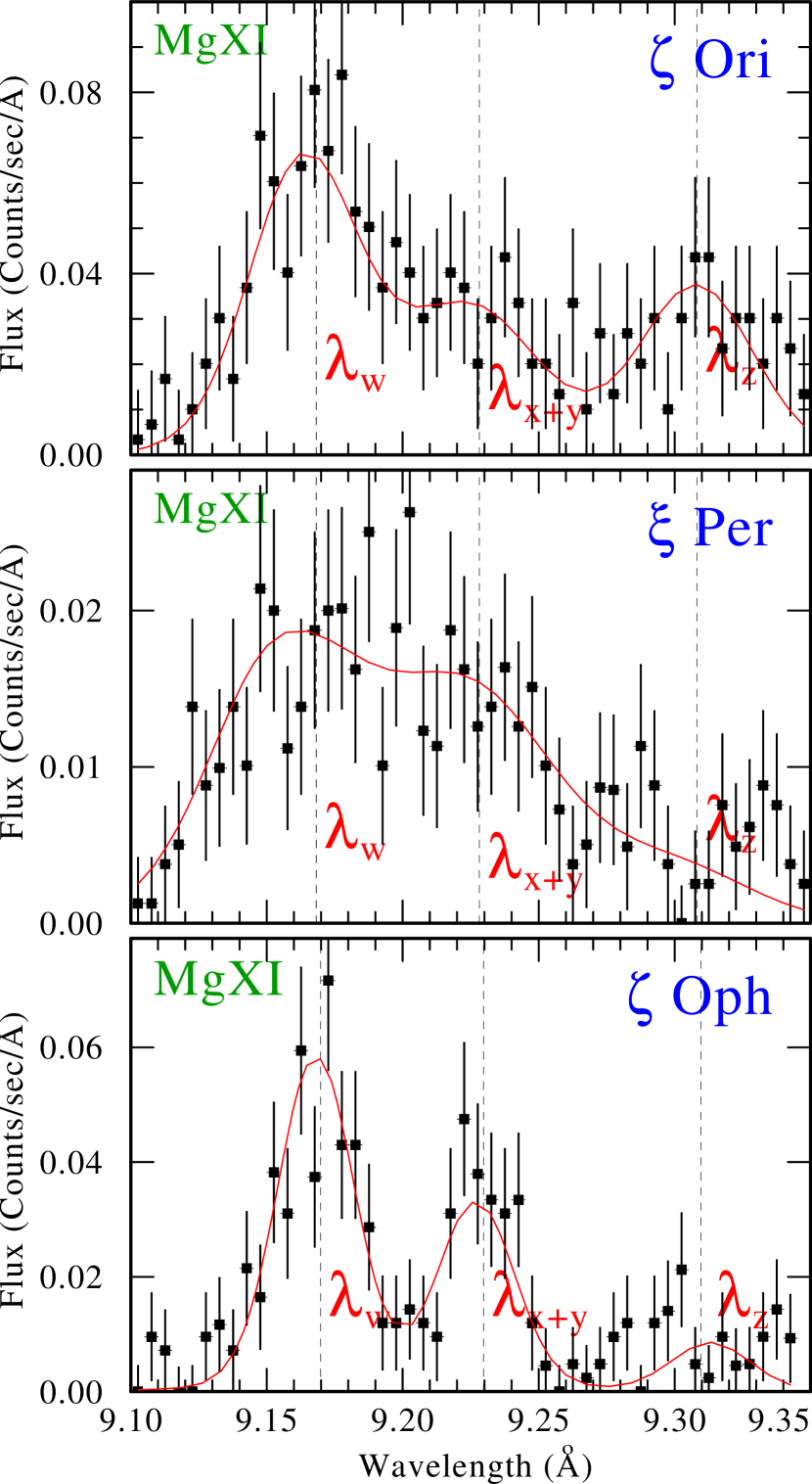
Figure 2: Mg xi line observed in the spectrum of $\zeta\,$Ori, $\xi\,$Per, and $\zeta\,$Oph (co-added meg$\pm 1$). Vertical dashed lines indicate rest-frame wavelength: $\lambda_{\rm w}$ – resonant line, $\lambda_{\rm x+y}$ – intercombination line, $\lambda_{\rm z}$ – forbidden line. The rest frame wavelengths in this and all following figures are corrected for the radial velocities taken from Hoogerwerf et al. (2001). The solid lines are triple-Gaussians fits.

We consider only single stars because in a CWB the geometry of the system can affect the line shapes (Henley, Stevens & Pittard 2003). However, there is no way to make sure that an O star is definitely single. Runaway O stars are distinguished by an almost complete lack of multiplicity (Hoogerwerf, de Bruijne & Zeeuw, 2001). Therefore, we have selected all three single O-type runaways observed by Chandra hetgs – $\zeta$ Pup, $\xi$ Per, and $\zeta$ Oph. These stars are relatively X-ray bright and observed with exposures long enough to accumulate high quality spectra as shown in Table 1 and in Fig. 1. We have also considered a fourth star, $\zeta$ Ori, albeit it is a known binary (Hummel et al., 2000), because the initial interpretation of X-ray emission line profiles from this star caused doubts in the validity of the shock model of X-ray production (Waldron & Cassinelli, 2001). The stellar and wind parameters of our sample stars are compiled in Table 2.

Waldron & Cassinelli (2001) and Cohen et al. (2006) presented a detailed analysis of Chandra observations of $\zeta$ Ori. Cassinelli et al. (2001) and Kramer et al. (2003) analyzed Chandra spectra of $\zeta$ Pup. XMM-Newton observations of $\zeta$ Pup were analyzed by Kahn et al. (2001) and Oskinova et al. (2006). Waldron (2005) reported observations of $\zeta$ Oph. Chandra observations of $\xi$ Per were not yet published to our knowledge.

We retrieved the public archival data of these four stars and extracted the spectra using the latest version of the Chandra software and the calibration data base. The de-reddened meg spectra of the stars are shown in Fig. 1 (see also XMM-Newton spectra of O stars in Fig. 8 from Paerels & Kahn (2003)). The emission lines seen in all spectra are resolved, with broader lines seen in the stars with higher wind velocities. The spectra exhibit emission from H-like and He-like ions of low and intermediate Z elements. The Si and Mg lines are most prominent in the $\zeta\,$Pup spectrum, while oxygen lines dominate the spectrum of $\zeta\,$Ori. The ratio of nitrogen to oxygen line fluxes is higher in the runaway stars compared to the $\zeta$ Ori spectrum. Kahn et al. (2001) found that in $\zeta\,$Pup the emission measures derived from the nitrogen emission lines are at least one order of magnitude larger that those of carbon and oxygen. They conclude that the elemental abundance ratios of nitrogen to oxygen, as well as nitrogen to carbon are considerably higher than solar indicating that the material has undergone CNO processing. This is in accordance with scenarios where runaways have previously been members of close binary systems and undergone mass exchange.

The spectral energy distribution (SED) of all stars can be fitted using the standard collisional plasma models, e.g. apec. The spectral fits indicate the presence of multi-temperature plasma with temperatures in the range $0.2\,{\rm keV}\raisebox{-1.72218pt}{$\stackrel{{\scriptstyle<}}{{\scriptstyle\sim}}$}kT_{\rm X}\raisebox{-1.72218pt}{$\stackrel{{\scriptstyle<}}{{\scriptstyle\sim}}$}0.7$ keV. Kahn et al. (2001) reported the detection of continuum in the XMM-Newton spectrum of $\zeta\,$Pup, although their fits were inconclusive. Oskinova et al. (2006) analyzed archival $\zeta\,$Pup data and concluded that the lines to continuum ratio is in agreement with the inferred plasma temperatures.

The emission lines seen in the spectra of O stars cannot be fitted by means of the stationary plasma emission line models implemented in the fitting software. The standard models are not adequate for the fast moving stellar winds, and cannot predict expected line profiles.

4 Line ratios for helium-like ions

Table 3: Ratios of fluxes^a in the components of He-like ions estimated by fitting observed spectral features.

Star	Ne ix		Mg xi		Si xiii
	R	G	R	G	R	G
$\zeta$ Pup	$0.35\pm 0.12$	$1.3\pm 0.3$	$0.36\pm 0.09$	$1.05\pm 0.15$	$0.9\pm 0.2$	$1.1\pm 0.2$
$\zeta$ Ori	$0.3\pm 0.2$	$0.9\pm 0.2$	$0.9\pm 0.4$	$1.1\pm 0.3$	$1.9\pm 1.6$	$1.4\pm 0.8$
$\xi$ Per	$0.1\pm 0.1$	$1.4\pm 0.5$	$0.19\pm 0.15$	$1.17\pm 0.35$	$2\pm 13$	$1\pm 3$
$\zeta$ Oph	$1.1\pm 1.1$	$1.13\pm 0.35$	$0.3\pm 0.1$	$1.0\pm 0.3$	$0.9\pm 0.8$	$0.6\pm 0.3$
a Fluxes are from the triple-Gaussian fitting of meg spectral lines

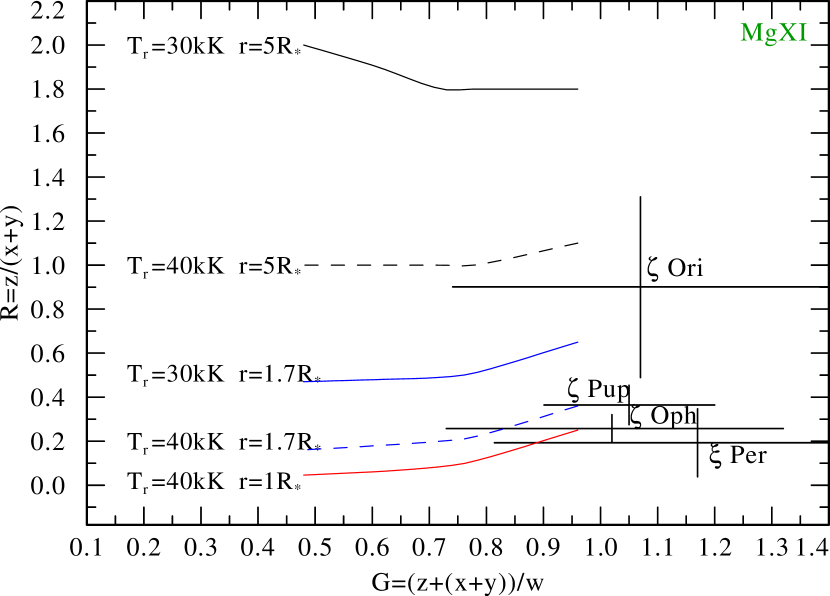
Figure 3: Observed and theoretical $R$ and $G$ ratios for the Mg xi fir triplet. Observed values are denoted by the star name. The curves represent the theoretical $R$ and $G$ from Porquet et al. (2001) for the corresponding $T_{\rm rad}$ and the radii of line formation. Observed values of $G$ are consistent with electron temperatures $T_{\rm e}\la 3$ MK. Observed values of $R$ roughly constrain the line emission regions between $\ga 1.5$ and $\la 5\,R_{*}$ for all stars.

The He-like ions show characteristic “fir triplets” of a forbidden ($z$), an intercombination ($x+y$) and a resonance ($w$) line. In OB type stars, the fir line ratios can be used to constrain the temperature and location of the X-ray emitting plasma. As was shown by Gabriel & Jordan (1969) the ratios $R(n_{\rm e})$ and $G(T_{\rm e})$ are sensitive to the electron density and to the electron temperature:

$$R(n_{\rm e},T_{\rm rad})=\frac{z}{x+y}$$ (1)

$$G(T_{\rm e})=\frac{z+(x+y)}{w}$$ (2)

A strong radiation field can lead to a significant depopulation of the upper level of the forbidden line via photo-excitation to the upper levels of the intercombination lines. This is analogous to the effect of electronic collisional excitation, thus mimicking a high density. For the characteristic densities of O star winds the photo-excitation is the dominant mechanism for depopulation. Since the radiation field dilutes with distance from the stellar surface, the ratio between forbidden and intercombination line provides information about the distance of the X-ray emitting plasma from the photosphere. However, this is possible only when the radiative temperature $T_{\rm rad}$ of the radiation field at the wavelength of the depopulating transition is known. Porquet et al. (2001) performed improved calculations of $R$ and $G$ line ratios for plasmas in collisional equilibrium and tabulated them for a wide range of parameters, including $T_{\rm rad}$.

Lines of O vii, Ne ix, Mg xi, and Si xiii are observed in all our sample stars, however O vii is well resolved only in $\zeta$ Oph. Therefore, we use in our analysis only He-like ions of Ne, Mg, and Si. In the sample stars with large wind velocities, $\zeta$ Pup and $\xi$ Per, the $w$, $x+y$, and $z$ components strongly overlap. Hence flux estimates in each separate component are ambiguous. The situation is best for $\zeta$ Oph, the star with the lowest wind velocity, where all components are well separated. To obtain the flux in the $w$, $x+y$, and $z$ components for a given ion, we have fitted all three components simultaneously as Gaussians. Figure 2 shows an example of the observed and fitted lines of a He-like ion. The derived $R$ and $G$ ratios for all stars are listed in Table 3.

The tables from Porquet et al. (2001) were used to constrain the temperature and location of the X-ray emitting plasma. The ratio $G$ is sensitive to $T_{\rm e}$, while it is almost insensitive to $n_{\rm e}$, $T_{\rm rad}$ and the dilution factor $W$. In our stars $G$ is large. The derived electron temperatures are lower than the temperatures corresponding to the ionisation potential for the given ion. The emission measures are highest for the ions with lowest ionisation potential. This is in accordance with the analysis of differential emission measure in $\zeta$ Pup and $\zeta$ Ori conducted by Wojdowski & Schulz (2005).

For electron densities less than $\sim 10^{12}$ cm^-3 and in the presence of a strong UV field, the ratio $R$ (forbidden to intercombination lines) is not sensitive to the density but depends instead on the electron temperature $T_{\rm e}$, radiative temperature $T_{\rm rad}$, and the dilution factor $W$. The electron temperature is constrained by $G$. The radiative temperature of the radiation field at the wavelength of interest (see Table 3 in Porquet et al. (2001)) can be determined from stellar atmosphere models. We employ PoWR model to calculate the radiation temperature as function of wavelength for different depth points in the wind. The radiative temperature at $\lambda_{{\rm f}\rightarrow{\rm i}}\,864\,$Å (Si xiii) as $\la 90$ per cent of the effective temperature. For the lighter ions $\lambda_{{\rm f}\rightarrow{\rm i}}\,1033\,$Å (Mg xi), $\lambda_{{\rm f}\rightarrow{\rm i}}\,1270\,$Å (Ne ix), the wavelength of interest is on the red side of the Lyman jump in the stellar SED, and the radiative temperature is higher, roughly equal to the effective temperature.

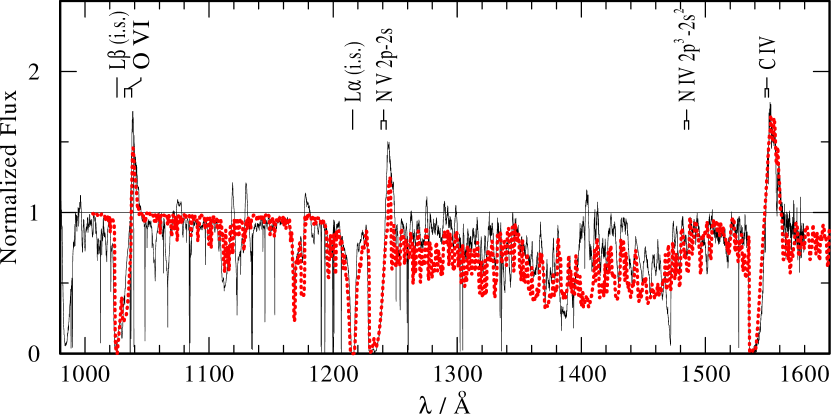
Figure 4: The EUV spectrum of $\zeta\,$Pup, observed with FUSE (thin line), compared to a PoWR model spectrum (dotted). The resonance doublets of C iv, N v and O vi are well reproduced, as well as the “forest” of iron-group lines. The O vi doublet can only be fitted with models when assuming that a diffuse X-ray field causes additional ionisation.

With $T_{\rm rad}$ and $T_{\rm e}$ constrained, the ratio $R$ can be used to estimate the dilution factor $W$ and, therefore, the radial distance $r$ from the stellar photosphere at which the X-rays are produced. The ratios $R$ and $G$ and corresponding error bars measured in Mg xi for our sample stars are shown in the $R-G$ diagram in Fig. 3. Theoretical values of $R$ and $G$, calculated by Porquet et al. (2001) for $T_{\rm rad}=30$ kK and $T_{\rm rad}=40$ kK, and for different distances $r$, are also plotted in Fig. 3. From comparison between observed and theoretical values of $R$ and $G$ we conclude that the Mg xi line is emitted by gas located between $1.5\,R_{*}$ and $5\,R_{*}$ in all stars. It should be noted, however, that the grids presented in Porquet et al. (2001) are quite coarse. Moreover, the observed lines, especially in $\xi\,$Per, are very noisy.

We constructed similar diagrams also for Ne ix and Si xiii. The latter line is sufficiently well resolved only in $\zeta$ Pup and $\zeta$ Oph. Comparison of $R-G$ diagrams for the different He-like ions in our sample stars allows to conclude that the X-ray emission originates not closer to the stellar photosphere than $\approx 1.5\,R_{*}$ and not further than $\approx 10\,R_{*}$, i.e. in the wind acceleration region for all stars of our sample.

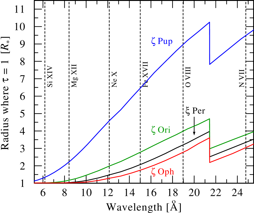
Figure 5: The radius were the radial optical depth of the wind becomes unity in dependence on the wavelength in the Chandra hetgs/meg range. The calculations were done using the PoWR stellar atmosphere code (see text) with stellar parameters from Table 2. The prominent edge at $\lambda\,21.5$ Å is due to oxygen. The vertical dashed lines correspond to the wavelengths of the studied lines (as indicated).

5 Mass-loss and stellar atmosphere models of sample stars

Full non-LTE stellar atmosphere models of O star winds are necessary to infer parameters of general, cool stellar wind. Recently, Puls et al. (2006) presented an up-to-date review of the effects of clumping on $\dot{M}$ determinations in O star winds. They analyzed H$\alpha$, IR, and radio fluxes of $\zeta\,$Pup and $\xi\,$Per (within a sample of 19 Galactic O stars) using non-LTE models which account for line-blanketing and clumping. The derived stellar parameters are listed in Table 2. The mass-loss rates are identical for H_α, IR, and radio determinations and constitute upper limits, since the clumping properties of the wind are still unknown (see Puls et al. (2006) for details). The stellar parameters for $\zeta\,$Oph listed in Table 2 are from Repolust et al. (2004). The mass-loss is based on the analysis of photospheric lines from H and He and shall be considered as an upper limit. This is also the case for parameters of $\zeta\,$Ori in Table 2 (Lamers et al., 1999).

The aim of this paper is to model the attenuation of X-rays in a clumped wind, where the photons are absorbed only in clumps and can escape freely between them. The total mass of the wind is conserved and distributed stochastically, in the form of clumps. The optical depth of clumps for the X-rays is determined by the wind density and the mass absorption coefficient. In our clumped model the total radial optical depth of the wind is absolutely the same as for a homogeneous wind of the same mass-loss rate.

We consider continuum absorption of X-rays in clumped cool wind caused predominantly by bound-free and K-shell ionisation processes. Introducing Cartesian coordinates, the $z$ axis points towards the observer and the impact parameter $p$ stands perpendicular to the latter. Alternatively, a point $(p,z)$ is specified by spherical coordinates, i.e. the radius $r=\sqrt{p^{2}+z^{2}}$ and the angle $\vartheta=\cos^{-1}\mu$ between the line of sight and the radial vector. Hence $\mu=z/r$. It is assumed that the time-averaged stellar wind is spherically symmetric and expands with a radius-dependent velocity

$$v(r)=v_{\infty}\left(1-\frac{r_{0}}{r}\right)^{\beta},$$ (3)

where $v_{\infty}$ is the terminal velocity, and $r_{0}$ is chosen such that $v(r\!=\!R_{\ast})=0.01\,v_{\infty}$. $R_{\ast}$ is the stellar (photospheric) radius. For a given mass loss rate $\dot{M}$, the continuity equation defines the density stratification via $\rho(r)=\mbox{$\dot{M}$}/(4\pi r^{2}v(r))$.

The wind can be specified by its total radial optical depth,

$$\tau_{\ast}=\int_{R_{*}}^{\infty}\kappa_{\nu}\rho(r)\ {\rm d}r\ ,$$ (4)

where $\kappa_{\nu}$ is the mass absorption coefficient, which describes the continuum opacity of the bulk of “cool” wind material at the frequency of the considered X-ray line.

In order to provide realistic values for this $\kappa_{\nu}$, we employ the Potsdam Wolf-Rayet (PoWR) model atmosphere code (Hamann & Gräfener, 2004). For each star we calculate a model with the parameters from Table 2, and the appropriate chemical composition from the references given in Table 2. For instance, enhanced nitrogen and depleted carbon and oxygen (Lamers et al., 1999) are taken for the $\zeta\,$Pup model. Figure 4 shows that our model spectrum of $\zeta\,$Pup agrees well with the observed EUV spectrum.

The O vi resonance doublet (see Fig. 4) can only be reproduced by models if there is a diffuse X-ray field causing some “superionisation”, as already recognized by Cassinelli & Olson (1979). In our model we adopt thermal bremsstrahlung emission from a hot embedded plasma component of $3\times 10^{6}$ K and adjust the filling factor such that the level of emerging X-rays corresponds roughly to the observation.

In fact, $\kappa_{\nu}$ chiefly depends on the chemical composition, but not much on other details of the model, nor on the radial coordinate. Table 4 gives $\kappa_{\nu}$ at the wavelength position of the studied X-ray emission lines, for each star of our sample. In order to visualize how opaque or transparent the stellar winds are for X-ray radiation, we plot at which radii the radial optical depth becomes unity (Fig. 5), for the wavelength range under consideration. At a few stellar radii, i.e. in the acceleration zone of the stellar wind where X-ray producing shocks should be located, the wind of $\zeta\,$Pup is optically thick for all considered X-ray lines (except perhaps Si xiv). In $\xi\,$Per and $\zeta\,$Ori, only the softer of the X-ray lines should encounter optically thick continuum absorption. The outer wind of $\zeta\,$Oph is almost transparent for the X-ray line photons.

6 Transfer of X-rays in a clumped stellar wind

Wind inhomogeneity alters the radiative transfer significantly. We have studied the effects of wind fragmentation on X-ray line formation analytically in the limit of infinitely many stochastically distributed fragments (Feldmeier et al., 2003), and numerically for a finite number of fragments within an accelerating stellar wind (Oskinova et al., 2004). The latter work describes in detail the model and the code used in the present paper. Here we briefly summarize the description of fragmented-wind opacity in order to introduce the parameters that will be used in the next section to model observed X-ray lines.

For a homogeneous wind, the optical depth $\tau_{\rm h}(p,z)$ between a point $(p,z)$ and the observer is

$$\tau_{\rm h}(p,z)=\frac{\kappa_{\nu}\mbox{$\dot{M}$}}{4\pi}\int_{z}^{\infty}\frac{{\rm d}z^{\prime}}{{r^{\prime 2}v(r^{\prime})}}\ .$$ (5)

with $r^{\prime}=\sqrt{p^{2}+z^{\prime 2}}$.

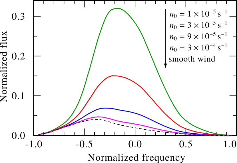
Figure 6: Solid lines: model line profiles of O viii in the spectrum of $\zeta$ Ori for different fragmentation frequency, $n_{0}$, as indicated. Dashed line: smooth wind model line. The line emission region is assumed between 1.5$R_{*}$ and 9$R_{*}$, velocity law is with $\beta=1$. Frequency is measured relative to the line center and in Doppler units referring to the terminal wind velocity $v_{\infty}$. Flux is normalized to the line flux in the unabsorbed case. All model lines in this paper are convolved with a Gaussian according to the hetgs/meg spectral resolution.

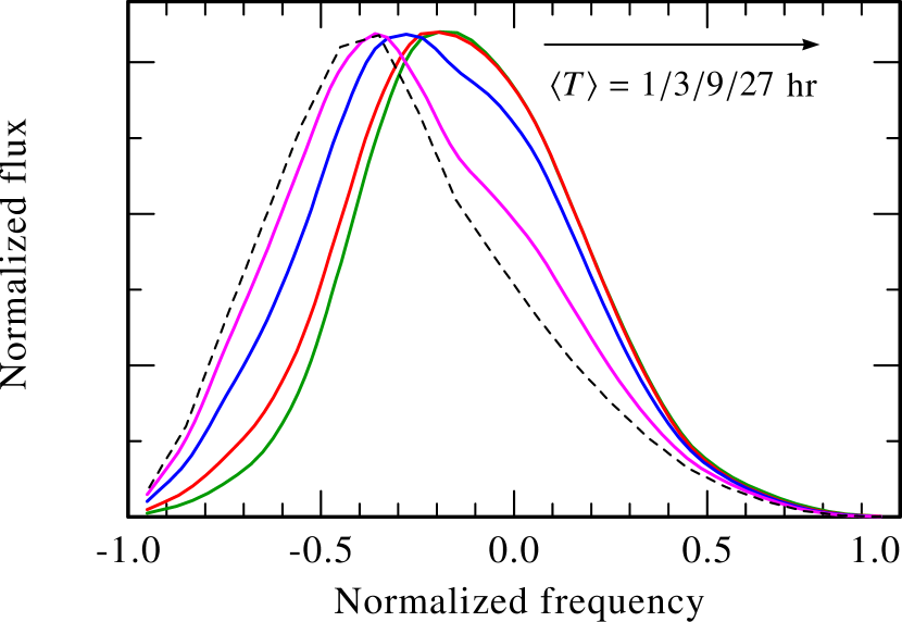
Figure 7: The same as in Fig. 6 but lines are normalized to the same maximum. The average time between subsequent clump passage, $\mathopen{<}T\mathopen{>}=1/n_{0}$, is indicated in the upper right corner.

We assume that close to the stellar core at distances smaller than $R_{\rm min}\la 1.5R_{*}$ the wind is homogeneous and no X-ray production is taking place. The wind instabilities start to develop at the distances larger than $R_{\rm min}$. These instabilities result in the heating of some small fraction of the material to X-ray emitting temperatures. The general stellar wind remains cool and is compressed into shell fragments. While general wind fragmentation persists till large distances $R_{\rm max}\approx 300R_{*}$, the X-ray emission is ceased at the distance $R_{\rm emis}\ga 5R_{*}$. We assume that the wind is homogeneous at distances $r\raisebox{-1.72218pt}{$\stackrel{{\scriptstyle>}}{{\scriptstyle\sim}}$}\,R_{\rm max}$ and take into account the absorption of X-rays by this part of the wind as well.

The hot material ($T_{\rm X}\sim 1$ MK) emitting X-rays is permeated with the cool ($T_{\rm w}\sim 10$ kK) wind fragments (i.e. clumps), which attenuate the X-ray emission. Both the hot and the cool gas component move outwards with the same velocity $v(r)$ and distributed stochastically.

We assume for simplicity that all parcels of gas which emit X-rays have the same temperature $T_{\rm X}$ and, on average, the same mass. The line emission is powered by collisional excitation and therefore scales with the square of the density. We assume that the hot gas parcels expand according to the continuity equation when propagating in radial direction. Hence, the emission of each hot parcel is $L_{0}/(r^{2}v(r))$, with a constant $L_{0}$ determined by the line emissivity.

The mass and the solid angle of each cool wind fragment are also preserved. In order that the time-averaged mass-flux $\dot{M}$  of shells resembles that of a stationary, homogeneous wind, the radial number density of shells must scale with $1/v(r)$:

$$n(r)=\frac{n_{0}}{v(r)}\ .$$ (6)

The parameter $n_{0}=n(r)v(r)$ defines the number of fragments passing through some reference radius (e.g. entering or leaving the wind) per unit of time and is constant due to the mass conservation. It does not depend on the distance and is therefore convenient model parameter. We refer to $n_{0}$ as the fragmentation frequency. The inverse quantity, $\mathopen{<}T\mathopen{>}$, is the average time interval between two consequent shells passing the same point in the stellar wind. When $\mathopen{<}T\mathopen{>}$ is equal to the flow time, $T_{\rm fl}=R_{*}/\mbox{$v_{\infty}$}$, the average separation between clumps is $1\,R_{*}$ when $v(r)=\mbox{$v_{\infty}$}$. In the wind acceleration region, where the X-rays are emitted, the radial separation between clumps is smaller. All model lines presented in this paper are computed assuming $n_{0}=T_{\rm fl}^{-1}$.

When $n_{0}$ is specified, the time averaged number of fragments in radial direction is

$$\langle N_{\rm r}\rangle=n_{0}\int_{R_{\rm min}}^{R_{\rm max}}\frac{{\rm d}r}{v(r)}.$$ (7)

As was discussed in Oskinova et al. (2004), the average radial optical depth of a fragment located at distance $r$ is

$$\bar{\tau}_{j}^{\rm rad}=\frac{\kappa_{\nu}\dot{M}}{4\pi}\cdot\frac{1}{r^{2}}\cdot\frac{1}{n_{0}}.$$ (8)

We assume here that the cool fragments are compressed radially and therefore aligned (this model sometimes is referred to as ”Venetian blinds”). The optical depth of a flattened fragment $j$ along line-of-sight depends on its orientation

$$\bar{\tau}_{j}=\frac{\bar{\tau}_{j}^{\rm rad}}{|\mu|},$$ (9)

where

$$|{\mu}|=\frac{z_{j}}{\sqrt{{p^{2}}+{z_{j}^{2}}}}.$$ (10)

Thus, the optical depth of each fragment, and therefore the effective wind opacity, is angular dependent. As discussed in Oskinova et al. (2004), the optical depth along the line of sight between point $(p,z)$ and the observer in a stellar wind which consists of aligned fragments is

$$\tau(p,z)=n_{0}\int_{z}^{z_{\rm max}}\ (1-{\rm e}^{-\bar{\tau}_{j}})\,|\mu(r^{\prime})|\,\frac{{\rm d}z^{\prime}}{v(r^{\prime})}+{\tau_{\rm h}(p,z_{\rm max})},$$ (11)

where $z_{\rm max}=\sqrt{R_{\rm max}^{2}-p^{2}}$, and ${\rm d}z^{\prime}={\rm d}r^{\prime}/\mu$. In the specific case of isotropic wind opacity, which was considered in Owocki & Cohen (2006), factor $\mu(r)$ in omitted in Eq. (9) and Eq. (11).

Let us compare the optical depth in a fragmented wind (Eq. 11) with the optical depth in a homogeneous wind (Eq. 5). In the limiting case of optically thin fragments ($\bar{\tau}_{j}^{\rm rad}\ll 1$) the exponent under the integral in Eq. (11) can be expanded. Substituting the average optical depth of a fragment defined by Eq. (9) the optical depth in the thin-fragment limit is the same as in a homogeneous wind.

The dependence of the model line on $n_{0}$ is demonstrated in Figs. 6,7. One can see from Eq. (8) that when $n_{0}$ is small the fragments are opaque for X-rays. In this case the radiation can escape only between fragments and the shape of the line profile does not change as long as the fragments remain opaque. With increasing $n_{0}$ the number of optically thin fragments increases, changing the line profile. For sufficiently large $n_{0}$, when all clumps are optically thin, the line profile looks like from the smooth wind model.

In the limit of optically thick fragments ($\bar{\tau}_{j}^{\rm rad}\gg 1$) the optical depth becomes

$$\tau(p,z)=n_{0}\int_{r}^{R_{\rm max}}\frac{{\rm d}r^{\prime}}{v(r^{\prime})},~{}~{}~{}\tau_{j}\gg 1\ ,$$ (12)

where the contribution from $\tau_{\rm h}(p,z(R_{\rm max}))$ is omitted for clarity.

The dependence of optical depth on the mass absorption coefficient $\kappa_{\nu}$ and $\dot{M}$ has disappeared in Eq. (12). Thus, in a limiting case of a wind which consists only of opaque fragments, the opacity is grey and is determined by the fragmentation frequency $n_{0}$ and the velocity.

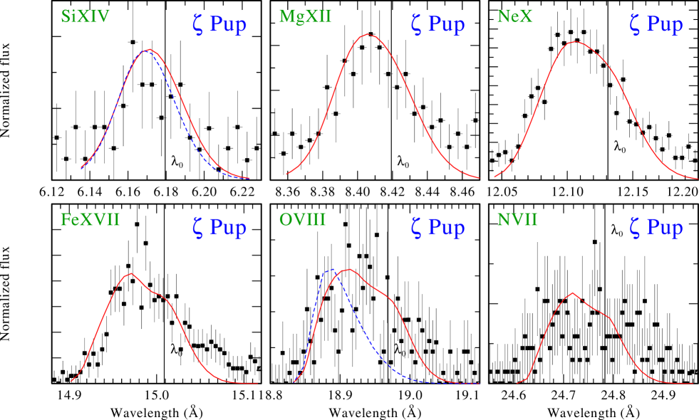
Figure 8: Strongest emission lines observed in $\zeta\,$Pup (co-added meg$\pm 1$) and the model lines. The solid lines are the model with $n_{0}=1.7\times 10^{-4}~{}{\rm s^{-1}}$ ($\mathopen{<}T\mathopen{>}=1.6$ hr), $\beta=0.9$, and the radiation originating between 1.5$R_{*}$ and 5$R_{*}$. The dashed line is for the homogeneous model of the same $\dot{M}$.

In our stochastic numeric wind model the fragments may have different optical depths, and are not necessarily opaque. As can be seen from Eq. (11) even when the optical thickness of the fragments is $\sim 1$ the dependence of optical depth $\tau(p,z)$ on $\kappa_{\nu}$ is weaker, compared to the homogeneous case (Eq. 5).

Hence, albeit the opacities $\kappa_{\nu}$ differ significantly depending on the wavelength (see Table 4), the optical depths $\tau(p,z)$ for different lines remains similar (more so in the case of optically thick clumps). Therefore the profiles of X-ray emission lines are similar across the spectrum.

7 Comparison with observed X-ray line profiles

Table 4: Mass absorption coefficient $\kappa_{\nu}$ [cm² g^-1] at the wavelengths of X-ray emission lines from stellar wind models, for the radial range between $1.5R_{*}$ and $5R_{*}$

Line	Wavelength [Å]	$\zeta$ Pup	$\zeta$ Ori	$\xi$ Per	$\zeta$ Oph
Si xiv	6.18	18	34	11	11
Mg xii	8.42	22	44	23	23
Ne x	12.14	59	73	55	57
Fe xvii	15.01	94	108	95	95
O viii	18.97	171	177	170	172
N vii	24.78	93	80	93	94

7.1 Model specification

The model is specified by mass-loss rate $\dot{M}$, velocity field parameters $v_{\infty}$ and $\beta$, mass-absorption coefficient $\kappa_{\nu}$, and fragmentation frequency $n_{0}$, as well as by the radii of the line emission zone.

We use the most recent published mass-loss rates for our sample stars. In case of $\zeta\,$Pup and $\xi\,$Per $\dot{M}$ is corrected for clumping, while for $\zeta\,$Ori and $\zeta\,$Oph the clumping is not accounted for. Velocity field parameters are from spectral analyses referenced in Table 2. The mass-absorption coefficients are determined using the sc PoWR code. For all our models we adopt the fragmentation frequency which is equal to the inverse wind flow time, $n_{0}=\mbox{$v_{\infty}$}/R_{*}$. The radii of the line emission zone are constrained from our analysis of fir line ratios in Sect. 4. Thus, no free parameter remains and a model is completely specified.

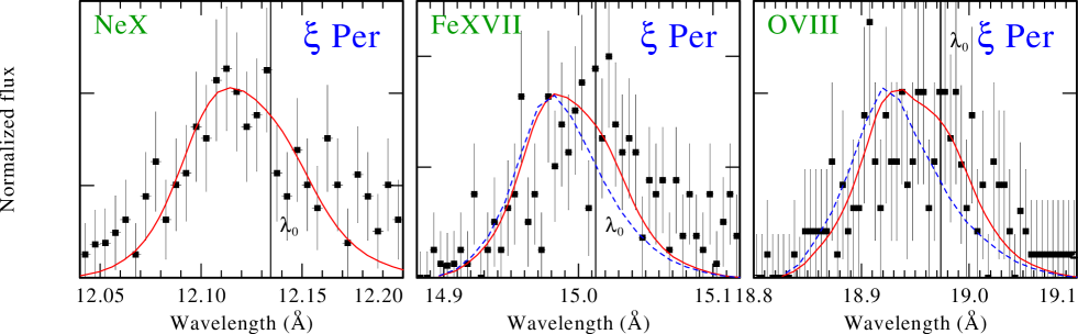
Figure 9: Lines of Ne x, Fe xvii, and O viii observed in $\xi\,$Per (co-added meg$\pm 1$) and the model lines. The solid lines are the model with $n_{0}=1.4\times 10^{-4}~{}{\rm s^{-1}}$ ($\langle T\rangle=1.9$ hr), $\beta=0.9$, and the radiation originating between 1.5$R_{*}$ and 7$R_{*}$. Dashed lines are homogeneous wind model.

7.2 X-ray emission lines in $\zeta\,$Pup, $\xi\,$Per, $\zeta\,$Ori, and $\zeta\,$Oph

$\zeta\,$Pup. Figure 8 shows the strongest emission lines observed in $\zeta\,$Pup. As can be seen in Fig. 5, the wind of $\zeta\,$Pup becomes optically thin for X-rays at the Si xiv $\lambda 6.18$  line just above 2$R_{*}$. When the wind is optically thin above the line emission region, the emergent line should be nearly symmetric relative to the rest wavelength $\lambda_{0}$. However, the peak of the Si xiv line is shifted to the blue, quite similar to other lines in Fig. 8. This indicates that the line photons must have originated below the surface of optical depth unity at $2R_{*}$. This is in agreement with the estimates based on the fir analysis.

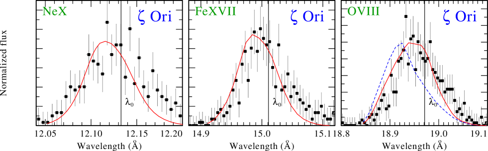
Figure 10: Lines of Ne x, Fe xvii, and O viii observed in $\zeta\,$Ori (co-added meg$\pm 1$) and the model lines. The solid lines are the model with $n_{0}=2.7\times 10^{-5}~{}{\rm s^{-1}}$ ($\mathopen{<}T\mathopen{>}=2.9$ hr ), $\beta=0.8$, and the radiation originating between 1.7$R_{*}$ and 9$R_{*}$. The dashed line is for the homogeneous model of the same $\dot{M}$.

The clumped wind model predicts that the shape of the emission lines is similar across the spectrum. This prediction is confirmed observationally. Kramer et al. (2003) note from the analysis of observed lines that the amount of absorption inferred for different lines in $\zeta\,$Pup and the line shapes are not sensitive to wavelength. We emphasize that the model lines shown in Fig. 8 are not selected best-fit models. These lines are computed using independently derived parameters. Comparing model and observation, we conclude that the stochastic wind model is capable to reproduce the observed lines sufficiently good.

Some of the lines shown in Fig. 8 are contaminated by blends. The N vii line is blended with N vi ($\lambda\,24.898$) (Pollock & Raassen, 2006). Similarly, Fe xvii line is possibly blended with Fe xix ($\lambda\,15.08$). Emission from O vii ($\lambda\,15.17$) is also likely to contribute in the far red wing of Fe xvii (Oskinova et al., 2006).

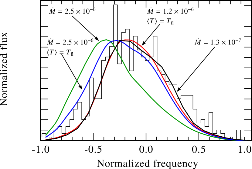
Figure 11: Observed (histogram) and model lines of O viii in $\zeta\,$Ori. Arrows indicate models used to compute the lines. For smooth wind models, only mass-loss rate, $\dot{M}\,[M_{\odot}\,{\rm yr}^{-1}]$ is shown, for clumped wind models, both mass-loss rate and the inverse fragmentation frequency, $\mathopen{<}T\mathopen{>}=n_{0}^{-1}$ is shown. Line with $\dot{M}=1.3\times 10^{-7}\,M_{\odot}\,{\rm yr}^{-1}$ is the best-fit smooth wind model, as found in Cohen et al. (2006).

$\xi\,$Per. The strongest X-ray emission lines observed in $\xi\,$Per  are shown in Fig. 9. The data are quite noisy, however, the lines look similar to each other regarding broadening and blue-shifts. For comparison, we have over-plotted on the Fe xvii and O vii line both smooth and fragmented model line profiles. The difference between them is relatively small, because the clumps in $\xi\,$Per  are not optically thick. It appears that the red wing of the Fe xvii line is above the model. This could be due to blending with lines from higher iron ions, or it may indicate that the fragmentation frequency is somewhat lower in $\xi\,$Per. Puls et al. (2006) suggest a much higher clumping factor in the outer wind of $\xi\,$Per than in $\zeta\,$Pup.

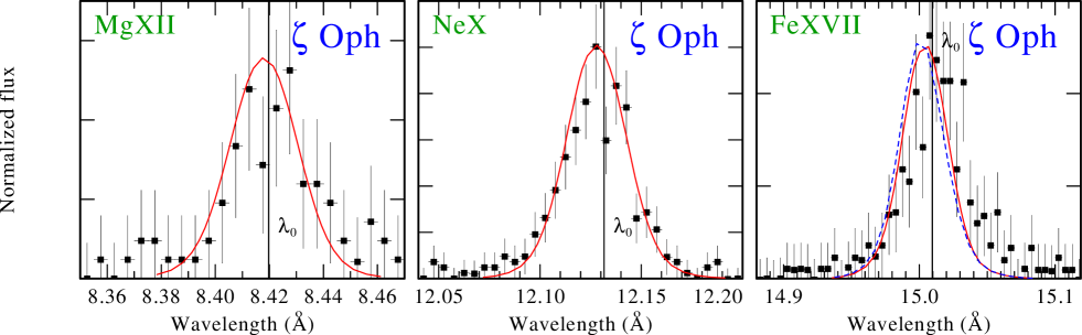
Figure 12: Lines of Mg xii, Ne x, and Fe xvii observed in $\zeta\,$Oph (co-added meg$\pm 1$) and the model lines. The solid lines are the model with $n_{0}=2.5\times 10^{-4}~{}{\rm s^{-1}}$  ($\mathopen{<}T\mathopen{>}=1.1$ hr), $\beta=1.5$, and the radiation originating between 1.5 $R_{*}$ and 9 $R_{*}$. The wind optical depth is smaller than unity for all these lines. Consequently, all lines can be equally well be reproduced by a smooth-wind model (shown by a dashed line).

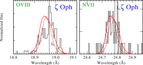
Figure 13: Lines of O viii and N vii observed in $\zeta\,$Oph (histograms, co-added meg$\pm 1$) and the model lines. The solid lines are from a model where radiation originates between 1.9 $R_{*}$ and 9 $R_{*}$, while dashed model lines are for the radiation from $1.5\,R_{*}-9\,R_{*}$.

$\zeta\,$Ori. Figure 10 shows the best-resolved lines in the $\zeta\,$Ori spectrum. The lines have similar shapes, they are blue-shifted and broadened. The model lines shown in Fig. 10 are calculated using mass-loss which is most certainly is overestimated by factor of $\sim$few. Therefore, the model lines are slightly shifted to the blue compare to the observed lines. As shown in Fig. 7, the reduction of fragmentation frequency by factor of 3 can shift the model line to the red by about $\approx 0.1\mbox{$v_{\infty}$}$. The reduction of empirical mass-loss rate of $\zeta\,$Ori will also lead to the improvement of the model. Lines of $\zeta\,$Ori were analyzed by Cohen et al. (2006) by means of smooth wind model. They have found from the best-fit model of O viii that $\kappa_{\nu}\dot{M}/4\pi\mbox{$v_{\infty}$}\approx 0.26$. Substituting the mass-absorption coefficient from Table 4 and stellar parameters from Table 2, the corresponding mass-loss rate is $\dot{M}\approx 1.3\times 10^{-7}\,M_{\odot}\,{\rm yr}^{-1}$, which is 20 times lower than estimated in Lamers & Leitherer (1993). On the other hand, the clumped wind model provides the same quality of fit assuming $\dot{M}$ only twice as low as in Table 2 and fragmentation frequency equal inverse flow time. This is illustrated in Fig. 11 which shows the observed and the four model lines of O viii in $\zeta\,$Ori. The line from clumped wind model, with $n_{0}=T_{\rm fl}^{-1}=9.1\times 10^{-5}\,{\rm s}^{-1}$ and $\dot{M}=1.2\times 10^{-6}\,M_{\odot}\,{\rm yr}^{-1}$ is nearly identical with the line computed using smooth wind model with $\dot{M}\approx 1.3\times 10^{-7}\,M_{\odot}\,{\rm yr}^{-1}$.

$\zeta\,$Oph. The wind of $\zeta\,$Oph is almost transparent for X-rays. As can be seen in Fig. 5, at the wavelengths of the Mg xii, Ne x and Fe xvii the wind is optically thin for the X-rays already above $\approx\,1.5\,R_{*}$. These lines are shown in Fig. 12. Due to the nearly complete lack of absorption in the wind the lines provide detailed information about the location and conditions of the hot plasma itself. The lines are symmetric and quite narrow, with broadening up to the $\pm$ 0.8 $v_{\infty}$. The slight asymmetry is due to occultation by the stellar core. The line shapes indicate that emission originates in the wind acceleration zone. The line shape is best reproduced (by eye estimate) when $\beta=1.5$. As can be seen from the two models over-plotted on the observed Fe xvii line, the difference between smooth and fragmented models is negligible for the thin wind of $\zeta\,$Oph.

At the wavelengths of the O viii and the N vii line the wind of $\zeta\,$Oph is thin only above $\approx\,2.5\,R_{*}$. These lines are shown in Fig. 13. Both these lines have a low signal-to-noise ratio, and it is difficult to assess the influence of wind absorption on line profiles. The O viii line appears asymmetric, with the blue wing being weaker than the red one, and our spherically-symmetric model cannot reproduce it well. However, it is not clear whether this line asymmetry is significant. The N vii line is slightly shifted to the blue. To demonstrate how sensitive is the emission line profile to the location of the X-ray emitting plasma, we show two model lines for O viii and N vii in Fig. 13. For each ion, the model lines differ only by the assumed minimum radii of X-ray emission. It appears that the O viii and the N vii lines originate from slightly further out in the wind than the lines shown in Fig. 12 at $\approx 1.9\,R_{*}$.

The $\zeta\,$Oph wind opacity is small and X-rays produced in the wind can escape without suffering significant attenuation. This allows to assess the intrinsic production of X-rays. We have calculated the ratios of the X-ray luminosity to the bolometric and mechanical ($\dot{M}v_{\infty}^{2}/2$) luminosity of stellar wind in $\zeta\,$Oph and compared it with these ratios for other stars. The results are given in Table 5.

The ratio of X-ray to bolometric luminosity in all stars in Table 5 is slightly smaller than the canonical $10^{-7}$ known for OB stars (Berghöfer et al., 1996). Perhaps, this is because the large sample of bright OB stars analyzed by Berghöfer et al. (1996) is biased towards binary stars, which tend to be more X-ray bright.

Table 5: Ratios of X-ray, bolometric and mechanical luminosities

Name	D	$L_{\rm X}$	$L_{\rm bol}$	$L_{\rm mech}$	$L_{\rm X}/L_{\rm bol}$	$L_{\rm X}/L_{\rm mech}$
	[pc]	[erg/s]	[erg/s]	[erg/s]
$\zeta$ Pup	460	$2.3\times 10^{32}$	$2.8\times 10^{39}$	$6.7\times 10^{36}$	$8.2\times 10^{-8}$	$3.4\times 10^{-5}$
$\zeta$ Ori	500	$2.1\times 10^{32}$	$3.0\times 10^{39}$	$3.5\times 10^{36}$	$6.8\times 10^{-8}$	$5.8\times 10^{-5}$
$\xi$ Per	850	$1.4\times 10^{32}$	$3.1\times 10^{39}$	$2.3\times 10^{36}$	$4.5\times 10^{-8}$	$6.0\times 10^{-5}$
$\zeta$ Oph	154	$1.2\times 10^{31}$	$2.8\times 10^{38}$	$\raisebox{-1.72218pt}{$\stackrel{{\scriptstyle<}}{{\scriptstyle\sim}}$}1.4\times 10^{35}$	$4.1\times 10^{-8}$	$\raisebox{-1.72218pt}{$\stackrel{{\scriptstyle>}}{{\scriptstyle\sim}}$}8.5\times 10^{-5}$
Distances are as used in papers quoted in Table 2

As can be seen from Table 5 the ratio of the X-ray and the mechanical luminosity is highest in $\zeta\,$Oph compared to the other stars with larger wind attenuation. We estimate that about 0.01% of the kinetic energy of the stellar wind of $\zeta\,$Oph is spent on the X-ray generation.

8 Discussion

The result of our analysis is that the stochastic wind model lines are in good agreement with the lines observed in stellar X-ray spectra. This confirms the clumped nature of O star winds.

So far, modern non-LTE stellar atmosphere models include clumping only in the first approximation of optically thin clumps. For clumps which are not optically thin, a non-LTE treatment requires to follow the transport of radiation inside the clumps, which is presently an impossible task at least in full detail.

But fortunately, the problem of X-ray formation in the winds of massive stars is much simpler, since we assume that the X-ray emission of optically thin plasma is decoupled from the continuum absorption in cool wind. Therefore, the full non-LTE treatment is not needed, and the solution of pure-absorption radiative transfer is sufficient.

Optically thin clumping in the winds reduces the empirically determined mass-loss rates. It is not a priory obvious how the presence of optically thick clumps may affect the mass-loss estimates (Brown et al., 2004). There is no observational evidence that the clumps in the wind are all optically thin. On the contrary, photometric and spectral variability indicate that opaque clumps are present in stellar winds. The outstanding question of “true“ stellar mass-loss rates in clumped winds is being extensively investigated at present (e.g. Puls et al., 2006).

8.1 On the dependence of line profiles on mass-loss rate

In our modeling we adopted mass-loss rates which, when available, account for the wind clumping. Since the mass is conserved in the wind, the optical depth in each clumps scales directly with $\dot{M}$, and inversely with fragmentation frequency (Eq. 8). The effect of wind clumping on the lines profiles is most pronounced when clumps are optically thick for the incident radiation (Feldmeier et al., 2003). Therefore, the reduction of empirical mass-loss rates means that in order for clumps to be optically thick the fragmentation frequency should be smaller.

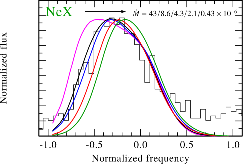
Figure 14: Observed (histogram, co-added meg$\pm 1$) and modeled Ne x line in $\zeta$ Pup. From left to right model line profiles are calculated  assuming $\mbox{$\dot{M}$}=43,\,8.6,\,4.3,\,2.1,\,0.43\times 10^{-6}M_{\odot}$ yr^-1. Corresponding normalization coefficient for the model line maximum to the observed line maximum is $\eta=2.6\times 10^{4},\,16.0,\,2.6,\,0.85,\,0.23$

In Fig. 14 we model the Ne x line in $\zeta\,$Pup for the same fragmentation frequency, but different mass-loss rates. The lowest value, $\mbox{$\dot{M}$}\approx 0.43\times 10^{-6}\,M_{\odot}\,{\rm yr}^{-1}$, is an estimate by Fullerton et al. (2006), based on the assumption that all phosphorus is in the P v ground level ($q({\rm P}^{4+})=1$). Adopting this value, the effect of wind absorption on the line profile is smaller than observered, as can be seen from the smaller blueshift of the model line compared to the observed line in Fig. 14. With increasing $\dot{M}$ the line maximum becomes more and more blueshifted.

The effect of increasing absorption on the line flux, which cannot be seen from Fig. 15 because the profiles are scaled to the same maximum, is dramatic. Actually, the profile for the highest $\dot{M}$ is $10^{5}$ times weaker than for the lowest $\dot{M}$, provided that the same flux has been originally released in the X-ray emitting zone. Even for the optically thin Fe xvii line in $\zeta\,$Oph (Fig. 12) the flux in the fragmented wind model is about 30% higher than that in the smooth wind model. Unfortunately, no models are available yet that would be able to predict the line fluxes based on detailed hydrodynamic simulations. A comparison of fluxes between modeled and observed lines would be a very sensitive tool.

8.2 On the influence of the velocity field on the line profile

The influence of the velocity field on model line profiles is illustrated in Fig. 15. Hydrodynamic simulations of Feldmeier et al. (1997) indicate that the velocity of the hot plasma is nearly the same as the cool-wind velocity. In this paper, we approximate the velocity field as monotonic ( see Feldmeier & Nikutta (2006) for the treatment of non-monotonic velocity). From the width of the line profiles we infer that the X-ray emission in all four stars is originating in a region extending from about $\approx 0.3$$v_{\infty}$ to $\approx 0.8$$v_{\infty}$. The corresponding radii of emission can be obtained if the velocity-law parameter $\beta$ is known. Vice versa, if radii of emission are given, $\beta$ can be inferred from the line-profiles. Usually, $\beta$ is estimated from UV line fits, and typically lies between 0.5 and 1.5. Fullerton et al. (2006) obtained for $\zeta\,$Pup $\beta=0.5$, while Puls et al. (2006) obtain $\beta=0.95$ and notice that different values may apply for inner and outer parts of the wind. $\beta\approx 1$ was inferred from the line profile variability in $\zeta\,$Pup (Eversberg et al., 1998). It seems that optical and UV line profiles are less sensitive to the exact value of $\beta$ than the X-ray lines studied here. As shown in Fig. 15, the line profile changes significantly in dependence on $\beta$. The synthetic lines for our four program stars shown in the figures were actually slightly optimized by adjusting $\beta$ within the uncertainties of previous estimates (see figure captions).

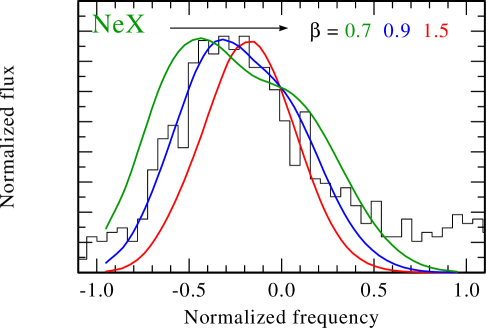
Figure 15: Observed (histogram, co-added meg$\pm 1$) and modeled Ne x line in $\zeta$ Pup. From left to right line profiles are calculated assuming $\beta=0.7,\,0.9,\,1.5$.

8.3 On the applicability of smooth wind radiative transfer in clumped winds

The optical depth in a smooth wind is given by Eq. (5), which was employed by Kramer et al. (2003) and Cohen et al. (2006) to fit the line profiles observed in the X-ray spectra of $\zeta\,$Pup and $\zeta\,$Ori. They have used $\tau_{0}=\kappa_{\nu}\mbox{$\dot{M}$}/4\pi v_{\infty}$ as one of their four free fitting parameters. Assuming $\kappa_{\nu}=125$ g cm^-2 for all analyzed lines in $\zeta\,$Ori, it was shown that the best-fitting values of $\tau_{0}$ imply significantly reduced mass-loss rates, e.g. due to the wind clumping. In a clumped wind, however, the optical depth is given by Eq. (11), which is more general than Eq. (5). The latter applies only for a limiting case of numerous and optically thin clumps.

Little is known so far about mass, density and geometry of individual clumps. Clump optical depths are likely to be different at different radii in the wind. This is reflected in our stochastic wind model, where the mass of a clump is conserved, but its radial optical depth scales as $r^{-2}$ (Eq. 8). Furthermore, since clump optical depth is proportional to $\kappa_{\nu}$, a clump can be optically thick at one wavelength and optically thin at another. As can be seen from Table 4, the mass absorption coefficient differs by one order of magnitude between the wavelenghts of the Si xiv and the O viii line. Figure 8 shows model lines of Si xiv and O viii in $\zeta\,$Pup. For the Si xiv line the difference between clumped and smooth model is small, indicating that the clumps are optically thin at $\lambda\,6.18$ (Si xiv). On the other hand, the model lines of O viii for smooth and clumped wind are significantly different, and, therefore, at least some fraction of the clumps are optically thick at $\lambda\,18.97$ (O viii). Consequently, Eq. (11) can be applied for the Si xiv line, but cannot be used for the O viii line.

Overall, when stellar mass-loss rates are revised down because of the wind clumping, the clumped wind radiative transfer should be applied for consistency.

8.4 On the line profiles and clump geometry

As discussed in detail in Oskinova et al. (2004), the optical depth in a clumped wind is determined by two factors. The first factor is the probability that a photon which encounters a clump is absorbed by clump material. This probability is obviously equal to one for optically thick clumps, $\tau_{\rm cl}\gg 1$, and is reduced otherwise to $1-\exp(-\tau_{\rm cl})$ (see Eq. 11).

The second factor is the probability that a photon propagating along the ray towards the observer does encounter a clump. When clumps are distributed randomly in the wind, this probability depends on the length of the path. The longer a photon travels through the wind, the higher is the probability that it will be intercepted by a clump. Therefore, photons emitted in the part of the wind which is receding from the observer have higher probability to be absorbed. Thus there are less photons in the red wing of a line reaching an observer than in the blue part. This is the basic physical reason for the blueshift of the X-ray emission line profiles.

Moreover, the probability that a photon does encounter a clump depends also on the clump cross-sections. Approximating clumps as spheres, the clump cross-section is the same from all directions, which is conceptually similar to the atomic cross-sections. The emergent line profiles are skewed in both cases.

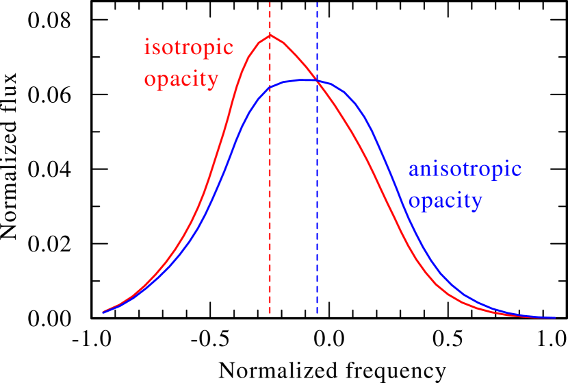
Figure 16: Two model lines, both calculated with $n_{0}=4.1\times 10^{-5}~{}{\rm s^{-1}}$ and $\tau_{0}=10$. Flux is normalized to the unabsorbed line flux. The only difference between the models is the assumption of isotropic opacity (i.e. clumps as “balls”) and anisotropic opacity (i.e. clumps as “pancakes”). The solid vertical lines mark the positions of line maxima. Isotropic opacity leads to a more blueshifted and significantly skewed line profile.

To explain the observed near-symmetry of line profiles in the framework of the smooth wind model, Kramer et al. (2003) and Cohen et al. (2006) suggested the reduction of mass-loss rates, which implies lower densities. When the particle number density is reduced, the photon mean free path is increased. In a clumped wind with spherical clumps, each clump is analogous to a particle. In order for the line profile to be symmetric, the “particle” (i.e. clump) number density must be reduced, which consequently leads to a larger photon mean free path (i.e. porosity length).

This deep analogy between smooth winds on one side and clumped winds with spherical clumps on the other side explains the principal similarity between the conclusions reached in Cohen et al. (2006) and in Owocki & Cohen (2006), namely the requirement of large mean free paths in order to produce symmetric emission line profiles.

A qualitatively different behavior of the radiative transfer is achieved, however, for anisotropic opacity (i.e. non-spherical, oriented clumps), as studied in Feldmeier et al. (2003) and Oskinova et al. (2004). This effect of clump geometry on emergent line profiles is demonstrated in Fig. 16. Two model lines are calculated with the the same fragmentation frequency and the same value of $\tau_{0}$. The only difference is that in one case isotropic opacity, i.e. spherical “ball-like” clumps are assumed, while the other model is calculated for the anisotropic opacity in the limiting case of clumps which are flat like “pancakes”. Figure 16 clearly shows that in the latter case the line is non-skewed and less blueshifted than in the former case.

The assumption of flat clumps was used in the present paper to model the observed line profiles. We have demonstrated that this model yields good agreement with the observed data.

9 Conclusions

The effect of clumping on the wind attenuation is threefold. Firstly, it reduces the wind absorption compared to the smooth-wind model, allowing for more flux to escape. Secondly, it leads to a weaker dependence of the effective opacity on wavelength, making it entirely grey in the case of optically thick clumps. This prediction of similar opacity for different lines agrees well with the similarity of line profiles observed at different wavelengths. Thirdly, it affects the shape of line profiles, but only in the case when effective anisotropic opacity is assumed. The radially compressed, slab-like shell fragments lead to the emergence of the symmetric, but blue-shifted lines profiles which are indeed observed.

Inhomogeneity of the stellar wind can reduce the mass-loss rates estimated empirically from the analysis of recombination and H$\alpha$ lines. These reduced mass-loss rates should be used in conjunction with the stochastic wind radiative transfer formalism in order to consistently model X-ray emission line profiles.

The radii in the wind where continuum optical depth for the X-rays is unity is below 10 $R_{*}$ in Chandra MEG energy band for $\zeta\,$Pup, $\zeta\,$Ori, $\xi\,$Per, and $\zeta\,$Oph. Stellar wind in $\zeta\,$Oph is almost transparent for the X-rays, consequently the emission line profiles show no effect of wind absorption. We estimate that $\sim\,0.01$% of the mechanical energy of the wind of $\zeta\,$Oph is converted into X-ray emission. The X-ray emission lines observed in the spectra of $\zeta\,$Pup, $\zeta\,$Ori,  and $\xi\,$Per are affected by wind absorption. This result, as well as shape of line profiles, is in agreement with the analysis of line ratios in the He-like ions. The above analysis constrains the origin of X-ray emission to the acceleration zone in the stellar wind.

Summarizing, we conclude that by using independently determined parameters as input for the model of an inhomogeneous stellar wind we are capable to reproduce the observed X-ray emission lines in O stars. The wind clumping explains the shape of the line profiles, i.e. their width, symmetry and blueshift, as well as their similarity across the spectrum.

References

- Berghöfer et al. (1996) Berghöfer T.W., Schmitt J.H.M.M., Cassinelli J.P., 1996, A&AS, 118, 481
- Bouret et al. (2005) Bouret J.-C., Lanz T., Hillier D.J., 2005, A&A, 438, 301
- Brown et al. (2004) Brown J.C., Cassinelli J.P., Li Q., Kholtygin A.F ., Ignace R. 2004, A&A, 426, 323
- Cassinelli & Olson (1979) Cassinelli, J.P. & Olson, G.L. 1979, ApJ, 229, 304
- Cassinelli et al. (2001) Cassinelli J.P., Miller N.A., Waldron W.L., MacFarlane J.J., Cohen D.H., 2001, ApJ, 554, L55
- Castor, Abbot & Klein (1975) Castor J.I., Abbott D.C., Klein R.I., 1975, ApJ, 195, 157
- Cohen et al. (2006) Cohen D.H., Leutenegger M.A., Grizzard K.T., Reed C.L., Kramer R.H., Owocki S.P, 2006, MNRAS, 368, 1905
- Dessart & Owocki (2003) Dessart L. & Owocki S.P., 2003, A&A, 406, L1
- Eversberg et al. (1998) Eversberg T., Lèpine S., Moffat A.F.J., 1998, ApJ, 494,799
- Feldmeier et al. (1997) Feldmeier A., Puls J., Pauldrach A.W.A., 1997, A&A, 322, 878
- Feldmeier et al. (2003) Feldmeier A., Oskinova L., Hamann W.-R., 2003, A&A, 403, 217
- Feldmeier & Nikutta (2006) Feldmeier,A. & Nikutta R., 2006, A&A, 446, 661
- Fullerton et al. (2006) Fullerton A.W., Massa D.L., Prinja R.K., 2006, ApJ, 637, 1025
- Gabriel & Jordan (1969) Gabriel A.H., & Jordan C., 1969, MNRAS, 145, 241
- Ignace (2001) Ignace R., 2001, ApJ, 549, L119
- Hamann & Koesterke (1998) Hamann W.-R. & Koesterke L., 1998, A&A, 335, 1003
- Hamann & Gräfener (2004) Hamann W.-R. & Gräfener G., 2004, A&A, 427, 697
- Harnden et al. (1979) Harnden F.R., Jr., et al., 1979, ApJ, 234, L51
- Henley et al. (2003) Henley D.B., Stevens I.R., Pittard J.M., 2003, MNRAS, 346, 773
- Hillier et al. (1993) Hillier D.J., Kudritzki R.P., Pauldrach A.W., Baade D., Cassinelli J.P., Puls J., Schmitt J.H.M.M., 1993, A&A 276, 117
- Hoogerwerf et al. (2001) Hoogerwerf R., de Bruijne J.H.J., Zeeuw P.T., 2001, A&A, 365, 49
- Hummel et al. (2000) Hummel C.A., White N.M., Elias II N.M., Hajian A.R., Nordgren T.E., 2000, ApJ, 540, L91
- Kahn et al. (2001) Kahn S.M., Leutenegger M.A., Cotam J., Rauw G., Vreux J.-M., den Boggende A.J.F., Mewe R., Güdel M., 2001, A&A, 276, 117
- Kramer et al. (2003) Kramer R.H., Cohen D.H., Owocki S.P., 2003, ApJ, 592, 532
- Lamers & Leitherer (1993) Lamers H.J.G.L.M. & Leitherer C, 1993, ApJ, 412, 771
- Lamers et al. (1999) Lamers H.J.G.L.M., Haser S., de Koter A., Leitherer C., 1999, ApJ, 516, 872
- Lucy & Solomon (1970) Lucy L.B. & Solomon P.M., 1970, ApJ, 159, 879
- MacFarlane et al. (1991) MacFarlane J.J., Cassinelli J.P., Welsh B.Y., Vedder P.W., Vallerga J.V., Waldron W.L., 1991, ApJ, 380, 564
- Markova et al. (2005) Markova N., Puls J., Scuderi S., Markov H., 2005, A&A, 440, 1133
- Miller et al. (2002) Miller N.A., Cassinelli J.P., Waldron W.L., MacFarlane J.J., Cohen D.H., 2002, ApJ, 577, 951
- Oskinova et al. (2004) Oskinova L.M., Feldmeier A., Hamann W.-R., 2004 A&A 422, 675
- Oskinova et al. (2006) Oskinova L.M., Hamann W.-R., Feldmeier A., 2006, in Proc. “High resolution X-ray spectroscopy: towards XEUS and Con-X”, astro-ph/0605560
- Owocki & Rybicki (1984) Owocki S.P. & Rybicki G.B., 1984, ApJ, 284, 337
- Owocki & Cohen (2006) Owocki S.P. & Cohen D.H., 2006, ApJ, in press (astro-ph/0602054)
- Paerels & Kahn (2003) Paerels F.B.S. & Kahn S.M., 2003, ARA&A, 41, 291
- Pollock et al. (2005) Pollock A.M.T., Corcoran M.F., Stevens I.R., Williams P.M., 2005, ApJ, 629, 482
- Pollock & Raassen (2006) Pollock A.M.T. & Raassen A., 2006, A&A , submitted
- Pomraning (1991) Pomraning G.C., 1991, Linear kinetic theory and particle transport in stochastic mixtures, Singapore; New Jersey: World Scientific. Series on advances in mathematics for applied sciences 7
- Puls et al. (2006) Puls J., Markova N., Scuderi S., Stanghellini C., Taranova O.G., Burnley A.W., Howarth I.D., 2006, A&A, 454, 625
- Porquet et al. (2001) Porquet D., Mewe R., Dubau J., Raassen A.J.J., Kaastra J.S., 2001, A&A, 376, 1113
- Repolust et al. (2004) Repolust T., Puls J., Herrero A., 2004, A&A, 415, 349
- (42) Runacres M.C. & Owocki S.P., 2005, A&A, 429, 323
- Sako et al. (2003) Sako M., Kahn S.M., Paerels F., Liedahl D.A., Watanabe S., Nagase F., Takahashi T., 2003, in High Resolution X-ray Spectroscopy with XMM-Newton and Chandra, ed. G. Branduari-Raymont (astro-ph/p309503)
- Schild et al. (2004) Schild H., et al., 2004, A&A, 422, 177
- Seward et al. (1979) Seward F.D., Forman W.R., Giacconi R., Griffiths R.E., Harnden F.R., Jr., Jones C., Pye J.P., 1979, ApJ, 234, L55
- Van der Meer et al. (2005) van der Meer A., Kaper L., Di Salvo T., et al., 2005, A&A, 432, 999