X-ray properties in massive galaxy clusters: XMM-Newton observations of the REFLEX-DXL sample

We selected an unbiased, flux-limited and almost volume-complete sample of 13 distant, X-ray luminous (DXL, $z\sim 0.3$) clusters and one supplementary cluster at $z=0.2578$ from the REFLEX Survey (the REFLEX-DXL sample). We performed a detailed study to explore their X-ray properties using XMM-Newton observations. Based on the precise radial distributions of the gas density and temperature, we obtained robust cluster masses and gas mass fractions. The average gas mass fraction of the REFLEX-DXL sample at $r_{500}$, $0.116\pm 0.007$, agrees with the previous cluster studies and the WMAP baryon fraction measurement. The scaled profiles of the surface brightness, temperature, entropy, gas mass and total mass are characterized by a self-similar behaviour at radii above 0.2–0.3 $r_{500}$. The REFLEX-DXL sample confirms the previous studies of the normalization of the scaling relations ($L$–$T$, $L$–$M$, $M$–$T$ and $M_{\rm gas}$–$T$) when the redshift evolution of the scaling relations is accounted for. We investigated the scatter of the scaling relations of the REFLEX-DXL sample. This gives the correlative scatter of (0.20,0.10) for variable of ($M$,$T$) of the $M_{500}$–$T$ relation, for example.

osmology: observations – Galaxies: clusters: general – X-rays: galaxies: clusters – (Cosmology:) dark matter

1 Introduction

The number density of galaxy clusters probes the cosmic evolution of large-scale structure (LSS) and thus provides an effective test of cosmological models. It is sensitive to the matter density, $\Omega_{\rm m}$, and the amplitude of the cosmic power spectrum on cluster scales, $\sigma_{8}$ (e.g. Schuecker et al. 2003). Its evolution is sensitive to the dark energy, the density of which is characterized by the parameter $\Omega_{\Lambda}$ and the equation of state parameter $w(z)$ (e.g. Vikhlinin et al. 2002; Allen et al. 2004; Chen & Ratra 2004).

The most massive clusters show the strongest and cleanest effects in the cosmological evolution. The structure of the X-ray emitting intra-cluster plasma in massive galaxy clusters is predominantly determined by gravitational effects and shock heating and is less affected by non-gravitational processes than low mass clusters. Only with decreasing cluster mass and intra-cluster medium (ICM) temperature, non-gravitational effects play an important role before and after the shock heating (Voit & Bryan 2001; Voit et al. 2002; Zhang & Wu 2003; Ponman et al. 2003). The X-ray properties of the most massive clusters are thus well described in hierarchical modeling. Therefore, massive galaxy clusters are especially important in tracing LSS evolution. The most massive clusters provide the cleanest results in comparing theory with observations.

Excluding cooling cores (Fabian & Nulsen 1977), a self-similar behaviour of the distributions of the ICM properties such as the temperature, density and entropy of massive clusters ($>$ 4 keV) is indicated in ROSAT, ASCA, Chandra and XMM-Newton observations (e.g. Markevitch 1998; Markevitch et al. 1998; Vikhlinin et al. 1999, 2005, 2006; Arnaud et al. 2002; Reiprich & Böhringer 2002; Zhang et al. 2004a, 2004b, 2005b; Ota & Mitsuda 2005; Pratt & Arnaud 2005; Pointecouteau et al. 2005) and simulations (e.g. Borgani 2004; Borgani et al. 2004; Kay 2004; Kay et al. 2004). As a consequence of the similarity, massive galaxy clusters show tight scaling relations such as the luminosity–temperature ($L$–$T$, e.g. Isobe et al. 1990; Markevitch 1998; Arnaud & Evrard 1999; Ikebe et al. 2002; Reiprich & Böhringer 2002), luminosity–mass ($L$–$M$, e.g. Reiprich & Böhringer 2002; Popesso et al. 2005), mass–temperature ($M$–$T$, e.g. Nevalainen et al. 2000; Finoguenov et al. 2001b; Neumann & Arnaud 2001; Xu et al. 2001; Horner 2001; Reiprich & Böhringer 2002; Sanderson et al. 2003; Pierpaoli et al. 2001, 2003), and luminosity–metallicity ($L$–$Z$, e.g. Garnett 2002) relations. Additionally, a reliable estimate of the intrinsic scatter of the scaling relations is the key to a correct modeling to constrain cosmological parameters in the cosmological applications using galaxy clusters. Therefore, understanding the intrinsic scatter of the scaling relations is as important as studying the scaling relations themselves. For example, on-going cluster mergers partially account for the scatter in the scaling relations since on-going mergers may lead to a temporary increase not only in the temperature and X-ray luminosity (Randall et al. 2002), but also in the core radius and slope of the surface brightness profile. Precise measurements of the ICM structure are required to allow accurate cluster mass and gas mass fraction determinations and thus to investigate the X-ray scaling relations for comparison of theory with simulations and observations.

The ROSAT-ESO Flux-Limited X-ray (REFLEX, Böhringer et al. 2001, 2004) galaxy cluster survey provides the largest homogeneously selected catalog of X-ray clusters of galaxies so far. It provides the basis to construct an unbiased sub-sample of clusters with specific selection criteria. We exploit it to compose a sample of distant, X-ray luminous (DXL) galaxy clusters in the redshift range, $z=0.27$ to $0.31$, with $L_{X}\leavevmode\nobreak\ \geq\leavevmode\nobreak\ 10^{45}\leavevmode\nobreak\ {\rm erg\leavevmode\nobreak\ s^{-1}}$ for the 0.1–2.4 keV band and one supplementary cluster at $z=0.2578$ (the REFLEX-DXL sample). The volume completeness correction can be done using the well known selection function of the REFLEX survey (Böhringer et al. 2004).

Prime goals for the study of the REFLEX-DXL sample are, (1) to obtain reliable ICM properties such as temperature structure (Zhang et al. 2004a, Paper II), (2) to determine accurate cluster masses and gas mass fractions using precise ICM property measurements, (3) to measure the normalization of the scaling relations with an improved accuracy and to discuss their intrinsic scatter in detail, and (4) to test the evolution of both the scaling relations and the temperature function (e.g. Henry 2004) by comparing the REFLEX-DXL sample (at $z\sim 0.3$) to nearby cluster samples. We present the results from high quality XMM-Newton data in this work. The data reduction is described in Sect. 2. We derive the X-ray properties of the ICM and determine the total masses and gas mass fractions based on precise gas density and temperature radial profiles in Sect. 3). We investigate the self-similarity of the REFLEX-DXL clusters (Sect. 4) and discuss the peculiarities of the individual clusters accounting for the scatter around the self-similarity (Sect. 5). In Sect. 6, we draw conclusions. Unless explicitly stated otherwise, we adopt a flat $\Lambda$CDM cosmology with the density parameter $\Omega_{\rm m}=0.3$ and the Hubble constant $H_{\rm 0}=70$ km s^-1 Mpc^-1. We adopt the solar abundance values of Anders & Grevesse (1989). Confidence intervals correspond to the 68% confidence level. We apply the Orthogonal Distance Regression method (ODR; e.g. Feigelson & Babu 1992; Akritas & Bershady 1996) and take into account measurement errors on both variables for the parameter fitting of the scaling relations. We use Monte Carlo simulations for the uncertainty propagation on all quantities of interest.

2 Data reduction

2.1 Data preparation

All 14 REFLEX-DXL clusters were observed by XMM-Newton in AO-1. Some properties of these observations and an overview of the sample are described in Böhringer et al. (2006, Paper I). The observations of 5 clusters in AO-1 were heavily contaminated by flares. Zhang et al. (2004a) investigated the temperature structure of 9 remaining REFLEX-DXL clusters observed in AO-1. Finoguenov et al. (2005) applied a 2-dimensional approach to study the structure such as projected density, temperature, pressure and entropy maps for those 9 REFLEX-DXL clusters. All 5 clusters flared in AO-1 were re-observed in AO-3 in which four have sufficient quality for a detailed study. All the clusters of the REFLEX-DXL sample were uniformly analyzed in this work.

All observations were performed with thin filter for three detectors. The MOS data were taken in Full Frame (FF) mode. The pn data were taken in Extended Full Frame (EFF) mode in AO-1 and FF mode in AO-3, respectively. For pn, the fractions of the out-of-time (OOT) effect are 2.32% and 6.30% for the EFF mode and FF mode, respectively. An OOT event file is created and used to statistically remove the OOT effect.

Good calibration is required for correct data reduction. The difference of the spectral measurements using low energy cut-off values of 1 keV and 0.4 keV was significant at the 1-$\sigma$ confidence level for most data sets in the previous analysis using the calibration in XMMSAS v5.4.0 (Zhang et al. 2004a). Now we use the XMMSAS v6.5.0 software for the data reduction. The new calibration in XMMSAS v6.5.0 provides a better agreement between data and model for EPIC, which are described in XMM-SOC-CAL-TN-0018 (Kirsch 2005). The CTI correction, point-spread function (PSF) core, astrometry, gain and energy redistribution have been improved. For example, in XMMSAS v6.0 the photon energy redistribution was strongly increased for energies below 0.53 keV in order to reduce excesses seen at low energies. Subsequent analysis of EPIC-pn spectra revealed large residuals around 0.43 keV which clearly showed that the redistribution was wrongly modeled in XMMSAS v6.0. The values in the redistribution matrix at low energies using the ground calibration were replaced based on the analysis of a set of spectra in the 0.1–2 keV band. For XMMSAS v6.5.0 the redistribution is performed energy-dependently to flattening the residuals. The spectra below 0.5 keV are greatly improved (Kirsch 2005). The spectral measurements using low energy cut-off values of 1 keV and 0.4 keV are now consistent for most REFLEX-DXL clusters except for RXCJ0658$-$5556 ($\sim$ 15%). With the new calibration in XMMSAS v6.5.0, we therefore use the 0.4–10 keV band for the spectral analysis.

Above 10 keV (12 keV), there is little X-ray emission from clusters for MOS (pn) due to the low telescope efficiency at these energies. The particle background therefore dominates. The light curve in the range 10–12 keV (12–14 keV) for MOS (pn), binned in 100 s intervals, is used to monitor the particle background and to excise periods of high particle flux. Since episodes of “soft proton flares” (De Luca & Molendi 2004) were detected in the soft band, the light curve of the 0.3–10 keV band, binned in 10 s intervals, is used to monitor and to excise the soft proton flares. A 10 s interval bin size is chosen for the soft band to provide a similar good photon statistic as for the hard band. The average and variance of the count rate (ctr) have been interactively determined for each light curve from the ctr histogram. Good time intervals (GTIs) are those intervals with ctrs below the threshold, which is defined as 3-$\sigma$ above the average. The GTIs of both the hard band and the soft band are used to screen the data. The background observations are screened by the GTIs of the background data, which are produced using exactly the same thresholds as for the corresponding cluster target field. All the observations of RXCJ2011.3$-$5725 were almost completely contaminated by flares. In total, 183 pn counts (0.4–10 keV) are available for the imaging spectral analysis of this cluster. RXCJ2011.3$-$5725 is therefore excluded in the detailed study. Settings of $FLAG=0$ and $PATTERN<13$ ($PATTERN<5$) for MOS (pn) are used in the screening process.

2.2 Source detection

Over half of the clusters show clear substructures or/and elongation. An “edetect_chain” command has been used to detect point-like sources. Point sources except for those suspicious candidates described below are subtracted before the further data reduction.

In the cluster center, point-like sources are hard to identify because their emission is blended with the strongly peaked cluster emission, in particular in cooling core clusters (CCCs). At the angular resolution of the observations, it is difficult to distinguish between a steep cooling core cusp and a central point source (e.g. an AGN in a central dominant galaxy). In principle, cluster emission is thermal and point source emission is non-thermal. The spectral shape can be used to identify point sources because a power law shape usually indicates the non-thermal emission contributed by point sources. We studied the spectra of the regions where there is a possible presence of point source in the cluster centers. We found that both “mekal” and “powerlaw” models provide acceptable fits. The photon statistic does not allow for a clear discrimination of the spectral shape. Therefore, a contribution of point sources to the cooling core cusp can not be ruled out for these clusters. The properties of these central regions are listed in Table  1. However, those suspicious candidates are not subtracted before the further data reduction.

2.3 Background subtraction

The background consists of several components exhibiting different spectral and temporal characteristics (e.g. De Luca & Molendi 2001; Lumb et al. 2002; Read & Ponman 2003). The background components can approximately be divided into two groups (e.g. Zhang et al. 2004a). Group I contains the background components showing significant vignetting (hereafter BVIGs), e.g. the cosmic X-ray background (CXB). Group II contains the components showing little or no vignetting (hereafter BNVIGs), e.g. particle-induced background.

It is safe to use a local background only if the vignetting effect is similar for the source and background regions. It becomes less reliable when large vignetting corrections are needed. The vignetting effect is energy-dependent and becomes significant above 5 keV. Additionally, the background component caused by the instrumental lines is different from position to position. This cannot be accounted for by a local background. The REFLEX-DXL cluster emission covers most of the field of view (FOV), $r\sim 8^{\prime}$. A local background is only available in the outskirts (e.g. $9.2^{\prime}<r<11.5^{\prime}$) but requires substantial vignetting corrections. When the local background is corrected for vignetting effects, the particle component is over corrected especially at high energies (artificially increased). This leads to an artificial softening of the derived cluster spectrum. The temperatures of the REFLEX-DXL clusters are above 5 keV, and thus tend to show a soft excess when the local background is used. Therefore, a local background is not the best choice for the analysis of the REFLEX-DXL sample.

Suitable background observations for such hot clusters are XMM-Newton observations of almost blank fields using the same instrumental set-up (e.g. a particular filter). We thus choose the blank sky accumulations in the Chandra Deep Field South (CDFS) as background. The CDFS observations used the same filter (thin filter for all detectors) and mode (FF/EFF mode for MOS/pn) as the REFLEX-DXL observations. In Zhang et al. (2005a), we investigated the blank sky accumulations in Lumb et al. (2002) as an alternative background and compared it to the CDFS observations. We found that the measurements are consistent within 1-$\sigma$ in both the spectral and the surface brightness analyses.

Suitable background observations guarantee similar BVIGs as for the targets in the same detector coordinates. One can subtract such a background extracted in the same detector coordinates as for the targets. However, the difference between the target and background should be taken into account as a residual background in the background subtraction. This can be done for the REFLEX-DXL clusters because the cluster X-ray emission does not cover the whole FOV, but the $r<9^{\prime}$ region. The outskirts in the FOV (e.g. $9.2^{\prime}<r<11.5^{\prime}$) were used to analyze the residual background. Strictly, the residual background, obtained after subtracting the blank field data, consists of both the residual CXB (because it varies on the sky) and the particle induced background (e.g residual background induced by soft protons).

2.4 Substructure

As an unbiased sample with respect to cluster morphology, the REFLEX-DXL clusters are characterized in terms of their dynamical state (Table 2, also see Zhang et al. 2006) using the classification in Jones & Forman (1992). The substructure consideration is based on the cluster morphology classification. The detection of the cluster morphology and substructures strongly depends on the cluster brightness, spatial resolution, and exposure time (Jones & Forman 1992). We define the substructure regions using the 0.5–2 keV image as follows.

As a start, we cut out the regions obviously contaminated by substructures. The remaining region can be fitted by a symmetric surface brightness model convolved with the PSF plus the scaled CDFS background. We simulated a 0.5–2 keV image by convolving the symmetric surface brightness model with the PSF plus the scaled CDFS background. We subtracted the simulated image from the observed 0.5–2 keV image and obtained a residual image. The summed counts of the substructure region in the residual image characterize the substructure signal ($S$). The summed counts of the same region in the simulated image are used as the background ($B$). We scaled the residual image using the simulated image and defined a series of contour regions. The signal-to-noise-ratio for each contour region was calculated by $S/N=S/\sqrt{S^{2}+B^{2}}$. The region corresponding to the $S/N>=1$ threshold is used to subtract the substructure. After point source subtraction and substructure excision, hydrostatic equilibrium should usually be valid in the remaining sector (more details see Sect. 5).

2.5 Spectral analysis

We use the XSPEC v11.3.1 software for the spectral analysis. A double background subtraction procedure can be applied in two ways in the spectral analysis. One approach was firstly described in Zhang et al. (2004a, 2005a, hereafter DBS I). The other method was well illustrated in Pratt & Arnaud (2002, hereafter DBS II). We applied both methods to perform the data reduction and obtained similar results using these two approaches.

For a given region of interest covering cluster emission, the spectrum is extracted from the background observations in the same detector coordinates as for the target. Both the response matrix file (rmf) and auxiliary response file (arf) are used to recover the correct spectral shape and normalization of the cluster emission component. The following is usually taken into account for the rmf and arf, (i) a pure redistribution matrix giving the probability that a photon of energy E, once detected, will be measured in data channel PI, (ii) the quantum efficiency (without any filter, which, in XMM-Newton calibration, is called closed filter position) of the CCD detector, (iii) filter transmission, (iv) geometric factors such as bad pixel corrections and gap corrections (e.g. around 4% for MOS), and (v) telescope effective area as a function of photon energy. The vignetting correction to effective area for off-axis observations can be accounted for either in the arf or in the event lists by a weight column created by “evigweight”.

In DBS I, the rmf corresponds to (i) and (ii), and the arf corresponds to (iii), (iv), (v) as well as the vignetting correction. A source spectrum is extracted from the outer region of the target observations. A background spectrum is extracted from the background observations in the same detector coordinates. Using only the rmf, the residual background spectrum is found after subtracting the background spectrum from the source spectrum in the outer region. We assume as an extreme case that the residual background mainly consists of the BNVIGs, e.g. soft protons. The vignetting effect can thus be ignored for the residual spectrum. It is modeled by a “powerlaw/b” model (“powerlaw/b” ,a power law background model which is convolved with the instrumental redistribution matrix but not with the effective area) in XSPEC limited to 0.4–15 keV. This model is used to account for the residual background in the spectral analysis over the whole energy range by applying a combined model of “wabs$*$mekal$+$powerlaw/b” (“mekal”, an emission model for hot diffuse gas, cf. Mewe et al. 1985, 1986; Arnaud & Rothenflug 1985; Arnaud & Raymond 1992; Kaastra 1992; Liedahl et al. 1995; “wabs”, a model considering the Galactic absorption) in XSPEC in the fitting procedure. The correct shape of the background component is recovered in the fit when the normalization of the “powerlaw/b” model is scaled to the area of the given region. The uncertainties of the fitting parameters of the “powerlaw/b” model are not introduced in the spectral analysis. This might result in an underestimate of the temperature uncertainty in the spectral analysis using DBS I. However, the advantage of DBS I is that the shape of the residual spectrum is conserved during the procedure.

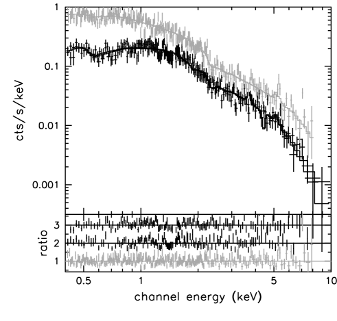
Figure 1: XMM-Newton spectra (pn in grey and MOS in black) of RXCJ0014.3$-$3022 of the 0.1–0.5 $r_{500}$ region fitted by the combined “wabs$*$mekal” model. The ratios of the observational data to the models are in the lower parts of the panels (offset zero for pn, $+1$ for MOS1, $+2$ for MOS2).

In DBS II, all spectra are extracted considering the vignetting correction by a weighted column in the event list produced by “evigweight”. The on-axis rmf and arf are co-created to account for (i) to (v). The target spectrum is extracted from the region of interest. The first-order background spectrum is given by a spectrum from the background observations which is extracted in the same detector coordinates as for the source spectrum, and which is scaled using the ctr ratio of the target and background limited to 10–12 keV (12–14 keV) for MOS (pn). The second-order background spectrum, the residual background spectrum, is prepared as follows. A source spectrum is extracted from the outer region of the target observations and its background spectrum from the same outer region of the background observations. The background spectrum is scaled using the ctr ratio of the target and background limited to 10–12 keV (12–14 keV) for MOS (pn), and is subtracted from the source spectrum to obtain a residual background spectrum. This residual background spectrum is normalized to the area of the region of interest as a second-order background spectrum. Both the first-order and second-order background spectra are subtracted from the target spectrum. A combined model of “wabs$*$mekal” is then used with the on-axis arf and rmf in XSPEC for the fitting (Fig. 1).

Basically, the vignetting correction is applied on the residual background in DBS II and not applied in DBS I. The former method is thus in principle better when the residual is dominated by the BVIGs (e.g. the CXB residual component), while the latter is better when the residual is dominated by the BNVIGs. The two approaches provide consistent results at the 1-$\sigma$ confidence level which indirectly tested the two approaches. A small discrepancy was found mostly in the last bin but showed no trend of being higher for one particular approach. There is no preferred indication of one of the two approaches. Additionally, the DBS II approach is simple in, (i) modeling the residual background, by applying the residual spectrum, instead of looking for an acceptable ($\chi^{2}<2$) power law model fit; (ii) allowing negative residual components, and (iii) generating one on-axis arf working for all the spectra extracted from different annuli. Therefore, we adopt the measurements using DBS II to illustrate the further computations.

2.6 Image analysis

The 0.5–2 keV band is used to derive the surface brightness profiles (also see Zhang et al. 2005a). This ensures an almost temperature-independent X-ray emission coefficient over the expected temperature range. The vignetting correction to effective area is accounted for using a weight column in the event lists created by “evigweight”. Geometric factors such as bad pixel corrections are accounted for in the exposure maps. The width of the radial bins is $2^{\prime\prime}$. An azimuthally averaged surface brightness profile of CDFS is derived in the same detector coordinates as for the targets. The ctr ratios of the targets and CDFS in the 10–12 keV band and 12–14 keV band for MOS and pn, respectively, are used to scale the CDFS surface brightness. The residual background in the 0.5–2 keV band is introduced by using the determined residual spectrum in the spectral analysis. The background-subtracted and vignetting-corrected surface profiles for three detectors are added into a single profile, and re-binned to reach a significant level of at least 3-$\sigma$ in each annulus. We take into account a 10% uncertainty of the scaled CDFS background and residual background.

2.7 PSF and de-projection

Using the XMM-Newton PSF calibrations by Ghizzardi (2001) we estimated the redistribution fraction of the flux. We found 20% for bins with width about $0.5^{\prime}$ and less than 10% for bins with width greater than $1^{\prime}$ neglecting energy dependent effects. The PSF blurring can not be completely considered for the spectral analysis as it is done for the image analysis because of the limited photon statistic. For such distant clusters, the PSF effect is only important within $0.3r_{\rm 500}$ and introduces an added uncertainty to the final results of the temperature profiles. This has to be investigated using deeper exposures with better photon statistic.

The projected temperature is the observed temperature from a particular annulus, containing in projection the foreground and background temperature measurements. Under the assumption of spherical symmetry, the gas temperature in each spherical shell is derived by de-projecting the projected spectra. In this procedure, the inner shells contribute nothing to the outer annuli. The projected spectrum in the outermost annulus is thus equal to the spectrum in the outermost shell. The projected spectrum in the neighboring inner annulus has contributions from all the spectra in the shell at the radius of this annulus and in the outer shells as shown in Suto et al. (1998). In XSPEC, a combined fit to the projected spectra measured in all annuli simultaneously gives the contribution of each spherical shell to each annulus and provides the de-projected measurements of the temperature and metallicity.

In the imaging analysis, we correct the PSF effect by fitting the observational surface brightness profile with a surface brightness model convolved with the empirical PSF matrices (Ghizzardi 2001). The surface brightness model is calculated by the projection of the radial electron density profile.

3 X-ray properties

The primary parameters of the REFLEX-DXL clusters are given in Table 3.

3.1 Density contrast

The mean cluster density contrast, $\Delta$, is the average density with respect to the critical density, $\rho_{\rm c}(z)=\rho_{\rm c0}E^{2}(z)$, where $E^{2}(z)=\Omega_{\rm m}(1+z)^{3}+\Omega_{\Lambda}+(1-\Omega_{\rm m}-\Omega_{\Lambda})(1+z)^{2}$. $r_{\Delta}$ is the radius within which the density contrast is $\Delta$. $M_{\Delta}$ is the total mass within $r_{\Delta}$. For $\Delta=500$, $r_{500}$ is the radius within which the density contrast is 500 and $M_{500}$ is the total mass within $r_{500}$.

3.2 Metallicity and temperature

We found that the X-ray determined redshifts agree with the optically measured redshifts (also in Zhang et al. 2004a). We therefore fixed the redshift to the optical redshift in the further analysis. The spectrum is fitted by a combined “wabs$*$mekal” model with fixed Galactic absorption (Dickey & Lockman 1990) and redshift (Böhringer et al. 2004a).

Temperature profiles can provide a useful means to study the thermodynamical history of galaxy clusters. XMM-Newton (and Chandra), in contrast to earlier telescopes, provides a less energy-dependent, and smaller, PSF. It is thus more reliable to study cluster temperature profiles with XMM-Newton. A systematic spectral analysis was performed in annuli. We re-binned the data to contain around 500–550 net counts per annulus for MOS1 in the 2–7 keV band. In XSPEC, a combined fit of “wabs$*$mekal$*$projct”to the projected spectra measured in all annuli simultaneously gives the contribution of each spherical shell to each annulus and provides the de-projected measurements of the temperature and also metallicity. In Fig. 2 we show the de-projected temperature profiles of the REFLEX-DXL clusters. The temperature profiles are approximated by the parameterization $T(r)=T_{3}\exp[-(r-T_{1})^{2}/T_{2}]+T_{6}(1+r^{2}/T_{4}^{2})^{-T_{5}}+T_{7}$ crossing all the data points. The temperature measure uncertainties are approximated by $T(r)\times(T_{8}+T_{9}r)$ and are propagated for individual data points by Monte Carlo simulations in the further analysis.

Vikhlinin et al. (2005) used the weighting of the 3-D temperature profile and averaged the temperature profile in a certain radial range. For the REFLEX-DXL sample, the radial temperature profiles are almost self-similar above 0.1–0.2$r_{500}$. The REFLEX-DXL data set shows significantly low $S/N$ above $0.5r_{500}$. Therefore, the volume averaged radial temperature profile of 0.1–0.5 $r_{500}$ is chosen as the global temperature $T$ listed in Table 3. Similarly, the metallicity profile of 0.1–0.5 $r_{500}$ is used to obtain the global metallicity $Z$ also listed in Table 3. We found an average of $0.24\pm 0.03$ $Z_{\odot}$ for the global metallicities of the REFLEX-DXL sample excluding RXCJ2011.3$-$5725. This agrees with the value of 0.21 $Z_{\odot}$ in Allen & Fabian (1998). It is also consistent with the averaged metallicity $\overline{Z}=0.21^{+0.10}_{-0.05}Z_{\odot}$ for 18 distant ($0.3<z<1.3$) clusters in Tozzi et al. (2003).

Based on the flared observations of RXCJ2011.3$-$5725, we measured a global spectral temperature ($\sim 4\pm 2$ keV) with a fixed metallicity of 0.3 $Z_{\odot}$ within $0.5^{\prime}$ radius.

3.3 Surface brightness

A $\beta$-model (e.g. Cavaliere & Fusco-Femiano 1976; Jones & Forman 1984) is often used to describe electron density profiles. To obtain an acceptable fit for all clusters in this sample, we adopt a double-$\beta$ model, $n_{\rm e}(r)=n_{\rm e01}(1+r^{2}/r_{\rm c1}^{2})^{-3\beta/2}+n_{\rm e02}(1+r^{2}/r_{\rm c2}^{2})^{-3\beta/2}$. The X-ray surface brightness profile model is linked to the radial profile of the ICM electron number density as an integral performed along the line-of-sight,

$$S_{\rm X}(R)\propto\int_{R}^{\infty}n_{\rm e}^{2}d\ell.$$ (1)

We fit the observed surface brightness profile by this integral convolved with the PSF matrices (Fig. 3) and obtain the parameters of the double-$\beta$ model of the electron density profile. The fit was performed within the truncation radius ($r_{\rm t}$, see Table 3) corresponding to a $S/N$ of 3 of the observational surface brightness profile. The truncation radii, $r_{\rm t}$, are about or above $r_{500}$ for the REFLEX-DXL clusters. The X-ray bolometric luminosity (here we use the 0.01–100 keV band) is given by $L_{\rm X}^{\rm bol}\propto\int\widetilde{\Lambda}(r)n^{2}_{\rm e}(r)dV$, practically an integral of the X-ray surface brightness to infinity (In practice, $20^{\prime}$ is used for the integral upper radial limit). We applied a power law to fit the surface brightness in the outskirts ($>0.4r_{500}$). More details about the slope of the the outskirts can be found in Sect. 5.1.

3.4 Cooling time

The cooling time is derived by the total energy of the gas divided by the energy loss rate

$$t_{\rm c}=\frac{2.5n_{\rm g}T}{n_{\rm e}^{2}\widetilde{\Lambda}}$$ (2)

where $\widetilde{\Lambda}$, $n_{\rm g}$, $n_{\rm e}$ and $T$ are the radiative cooling function, gas number density, electron number density and temperature, respectively. We compute the upper limit of the age of the cluster as an integral from the cluster redshift $z$ up to $z=100$. Cooling regions are those showing cooling time less than the upper limit of the cluster age. The boundary radius of such a region is called the cooling radius. The cooling radius is zero when the cooling time is larger than the cluster age. The cooling times and cooling radii are given in Table 4.

3.5 Gas entropy

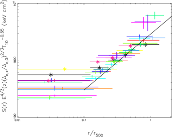
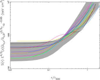
Figure 10: Left: Scaled entropy profiles and the best fit of the $r>0.1r_{500}$ region. The merger clusters (RXCJ0014.3$-$3022, RXCJ0516.7$-$5430 and RXCJ2337.6$+$0016) are shown with asterisk symbols. $T_{10}$ denotes temperatures in units of 10 keV. Right: Scaled entropy profile fits of the REFLEX-DXL sample compared to the Birmingham-CfA clusters (grey shadow) in a temperature range of 6–20 keV. The colours have the same meaning as those in Fig. 4.

The entropy is the key to an understanding of the thermodynamical history since it results from shock heating of the gas during cluster formation. The observed entropy is generally defined as $S=Tn_{\rm e}^{-2/3}$ for galaxy cluster studies (e.g. Ponman et al. 1999), and it scales with the cluster temperature. An excess above the scaling law indicates non-gravitational heating effects by sources such as the feedback from super-novae (SN) and AGNs (e.g. Lloyd-Davies et al. 2000). Radiative cooling can also raise the entropy of the ICM (e.g Pearce et al. 2000) or produce a deficit below the scaling law. In this sample, the clusters appearing more relaxed are identical to those showing lower central entropy values. For the REFLEX-DXL clusters, the most inner temperature data points are measured at $\sim 0.1r_{500}$. This leads to the fact that the entropies at $0.1r_{500}$ ($S_{\rm 0.1r_{500}}$) are resolved and can be used as the values of the central entropies as shown in the entropy radial distributions (Fig. 10). At $0.1r_{200}$ (about $0.18r_{500}$), the entropy increases as a function of radius and is thus significantly larger than the central entropy.

3.6 Mass distribution

We assume that the intra-cluster gas is in hydrostatic equilibrium within the gravitational potential dominated by DM. The ICM can thus be used to trace the cluster potential. Under the assumption of spherical symmetry, the cluster mass is calculated from the X-ray measured ICM density and temperature distributions,

$$\frac{1}{\mu m_{\rm p}n_{\rm e}(r)}\frac{d[n_{\rm e}(r)T(r)]}{dr}=-\frac{GM(<r)}{r^{2}}\leavevmode\nobreak\ ,$$ (3)

where $\mu=0.62$ is the mean molecular weight per hydrogen atom. Following the Monte Carlo simulation method (e.g. Neumann & Böhringer 1995), we use a set of input parameters of the approximation functions, in which $\beta$, $n_{\rm e0i}$, $r_{\rm ci}$ ($i=1,2$) are for the gas density radial profile $n_{\rm e}(r)$ and $T_{\rm i}$ ($i=1,...,7$) are for the temperature radial profile $T(r)$, respectively, to compute the cluster mass. The individual data point uncertainties are propagated by Monte Carlo simulations. We used the measured mass profile to estimate $M_{500}$ and $r_{500}$.

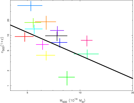
Figure 6: The concentration parameter of the extended-NFW model versus mass for the REFLEX-DXL sample. The line denotes the best fit of the REFLEX-DXL sample. The colours have the same meaning as those in Fig. 4.

The NFW model (e.g. Navarro et al. 1997, 2004, NFW) cannot provide an acceptable fit for the observed mass profiles. We therefore adopt the best fit of an extended-NFW model (e.g. Hernquist 1990; Zhao 1996; Moore et al. 1999), $\rho_{\rm DM}(r)=\rho_{\rm s}(r/r_{\rm s})^{-\alpha}(1+r/r_{\rm s})^{\alpha-3}$, where $\rho_{\rm s}$ and $r_{\rm s}$ are the the characteristic density and scale of the halo, respectively. In Fig. 5, we show the measured mass profiles and their best extended-NFW model fits. We derive the concentration parameters ($c_{500}$) of the DM distributions of the REFLEX-DXL clusters (see Table 5) using the extended-NFW model. The difference in the concentration parameters using different models can be large. For instance, an extended-NFW profile fitted to the numerical simulations of Moore et al (1999) gives a concentration parameter 50% higher than the concentration parameter given by the NFW model. In general, the theoretical and observed concentration–mass relations are compared when the same models (e.g. NFW) are considered. However, the REFLEX-DXL data cannot be well fitted by the NFW model. We thus cannot directly compare our results to the published observations (e.g. Pointecouteau et al 2005) and simulations (e.g. Dolag et al. 2004) which are based on the NFW model. The best fit of the REFLEX-DXL sample gives the slope of $1.5\pm 0.2$ and the normalization of $10^{2.1\pm 0.2}$ (Fig. 6). If we fixed the slope parameter to $-0.102$ for the concentration–mass relation as found in Dolag et al. (2004), the best fit of the REFLEX-DXL sample gives the normalization of $8.7\pm 7.8$.

3.7 Gas mass fraction distribution

The gas mass fraction is an important parameter for cluster physics, e.g. heating and cooling processes, and cosmological applications using galaxy clusters (e.g. Vikhlinin et al. 2002; Allen et al. 2004). The gas mass fraction distribution is defined to be $f_{\rm gas}(<r)=M_{\rm gas}(<r)/M(<r)$.

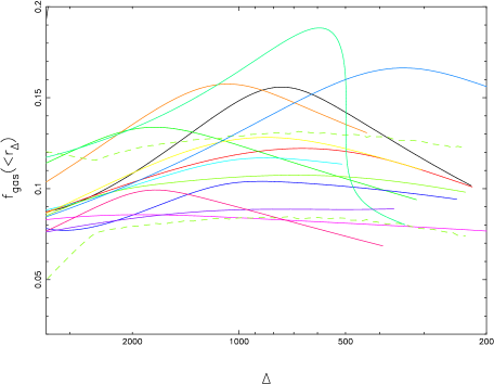
Figure 7: Gas mass fraction as a function of density contrast for the REFLEX-DXL sample. The 1-$\sigma$ error corridor (dashed curves) is displayed for RXCJ0532.9$-$3701 only. The colours have the same meaning as those in Fig. 4.

As shown in Fig. 7, the gas mass fractions increase as a function of radius in the $r_{3000}<r<r_{1000}$ region. This indicates that the DM distribution is more concentrated in the center than the gas distribution. We derived an average gas mass fraction of $0.116\pm 0.007$ at $r_{\rm 500}$. This agrees with the gas mass fractions found for many massive clusters showing temperatures greater than 5 keV (e.g. Mohr et al. 1999). The gas mass fractions around $r_{2500}$ show the smallest scatter, $0.100\pm 0.007$, and the values are similar to the measurements of Allen et al. (2002) based on Chandra observations of 7 clusters yielding $f_{\rm gas}\sim 0.105$–$0.138h^{-3/2}_{70}$. At $r_{200}$, the extrapolated gas mass fractions show consistency with the measurements of Sanderson et al. (2003) based on ASCA/GIS, ASCA/SIS and ROSAT/PSPC observations of 66 clusters yielding $f_{\rm gas}=0.13\pm 0.01h^{-3/2}_{70}$, the measurements of Ettori et al. (2002a) based on BeppoSAX observations of 22 nearby clusters, and the gas mass fraction for A1413 (Pratt & Arnaud 2002) at $z=0.143$ based on XMM-Newton observations yielding $f_{\rm gas}\sim 0.12h^{-3/2}_{70}$. As expected, the gas mass fraction distributions of the REFLEX-DXL clusters are lower than the universal baryon fraction, $f_{\rm b}=\Omega_{\rm b}/\Omega_{\rm m}=0.167\pm 0.014$, based on the recent WMAP measurements, $h=0.71^{+0.04}_{-0.03}$, $\Omega_{\rm b}\leavevmode\nobreak\ h^{2}=0.022\pm 0.001$ and $\Omega_{\rm m}\leavevmode\nobreak\ h^{2}=0.132^{+0.008}_{-0.009}$ (e.g. Spergel et al. 2003; Hansen et al. 2004). This is because the baryons in galaxy clusters reside mostly in hot gas together with a fraction (15% $f_{\rm gas}$) in stars as implied from simulations (e.g. Eke et al. 1998; Kravtsov et al. 2005). In principle, $\Omega_{\rm m}$ can be determined from the baryon fraction, $f_{\rm b}=f_{\rm gas}+f_{\rm gal}$, in which a contribution from stars in galaxies is given by $f_{\rm gal}=0.02\pm 0.01h_{50}^{-1}$ (White et al. 1993). The gas mass fractions, $\sim 0.116\pm 0.007$, at $r_{500}$ of the REFLEX-DXL clusters support a low matter density Universe as also shown in recent studies (e.g. Allen et al. 2002; Ettori et al. 2003; Vikhlinin et al. 2003).

4 Scaling relations

Simulations (e.g. Navarro et al. 1997, 2004) suggest a self-similar structure for galaxy clusters in hierarchical structure formation scenarios. The scaled profiles of the X-ray properties and their scatter can be used to quantify the structural variations. This is a probe to test the regularity of galaxy clusters and to understand their formation and evolution. The accuracy of the determination of the scaling relations, limited by how precise the cluster mass and other global observable can be estimated, is of prime importance for the cosmological applications of clusters of galaxies.

Because the observational truncation radii ($r_{\rm t}$) in the surface brightness profiles are about or slightly above $r_{500}$, we use $r_{500}$ for radial scaling.

The following redshift evolution corrections (e.g. Ettori et al. 2004) are usually used to check the dependence on the evolution of the cosmological parameters,

$S_{\rm X}\cdot E^{-3}(z)\;(\Delta_{c,z}/\Delta_{c,0})^{-1.5}\propto f(T)$,

$S\cdot E^{4/3}(z)\;(\Delta_{c,z}/\Delta_{c,0})^{2/3}\propto f(T)$,

$L\cdot E^{-1}(z)\;(\Delta_{c,z}/\Delta_{c,0})^{-0.5}\propto f(T)$,

$M\cdot E(z)\;(\Delta_{c,z}/\Delta_{c,0})^{0.5}\propto f(T)$,

$M_{\rm gas}\cdot E(z)\;(\Delta_{c,z}/\Delta_{c,0})^{0.5}\propto f(T)$,

where $\Delta_{\rm c,z}=18\pi^{2}+82[\Omega_{\rm m,z}-1]-39[\Omega_{\rm m,z}-1]^{2}$ for a flat Universe and $\Omega_{\rm m,z}$ is the cosmic density parameter at redshift $z$.

4.1 Scaled temperature profiles

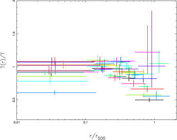
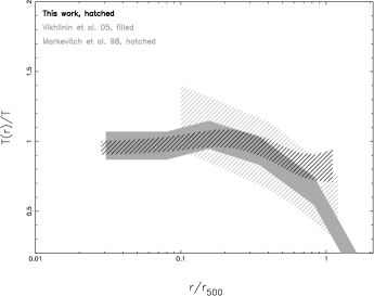
Figure 8: Left: Scaled radial temperature profiles. The colours have the same meaning as those in Fig. 4. Right: An average temperature profile of the REFLEX-DXL clusters compared to the temperature profile ranges in Markevitch et al. (1998, grey, hatched) and Vikhlinin et al. (2005, grey, filled).

Studies of the cluster temperature distributions (e.g. Markevitch et al. 1998; De Grandi & Molendi 2002) indicate a steep decline beyond an isothermal center. We scaled the radial temperature profiles by the global temperature $T$ and $r_{500}$ as shown in Fig. 8. An average temperature profile is derived by averaging the 1-$\sigma$ boundary of the scaled radial temperature profiles of the REFLEX-DXL clusters. As shown in Fig. 8, we found a closely self-similar behaviour. Up to $0.3r_{\rm 500}$, we observed an almost constant temperature distribution with a temperature peak at around 0.2 $r_{\rm 500}$. Four clusters (RXCJ0232.2$-$4420, RXCJ0307.0$-$2840, RXCJ0437.1$+$0043 and RXCJ0528.9$-$3927) show relatively cool cluster cores. A temperature profile decreasing down to 80% of the peak value has been observed outside $0.3r_{\rm 500}$ for the average of the REFLEX-DXL clusters. Three clusters (RXCJ0437.1$+$0043, RXCJ0658.5$+$5556, and RXCJ2308.3$+$0211) show temperatures rising with relatively large error bars in their temperature profiles. The average temperature profile can decline down to 50% of the peak value when these three clusters are excluded. This average temperature profile is consistent with the average profiles from ASCA in Markevitch et al. (1998), BeppoSAX in De Grandi & Molendi (2002) and Chandra (using an assumed uncertainty of 20% of the averaged temperature profile as an approximate illustration) in Vikhlinin et al. (2005) within the observational dispersion. A similarly universal temperature profile is indicated by simulations (e.g. Borgani et al. 2004; Borgani 2004).

4.2 Scaled surface brightness profiles

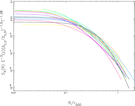
Figure 9: Surface brightness profile fits scaled according to the empirical scaling, $S_{\rm X}\propto T^{1.38}$ given in Arnaud et al. (2002). The colours have the same meaning as those in Fig. 4.

We scaled the surface brightness profiles using the self-similar scaling, $S_{\rm X}\propto T^{0.5}$, and the empirical scaling, $S_{\rm X}\propto T^{1.38}$, respectively, as described in e.g. Arnaud et al. (2002). Both scaled profiles show a less scattered self-similar behaviour at $r>0.2r_{500}$ (see Fig. 9). The core radii populate a broad range of values, 0.03–0.2 $r_{500}$.

4.3 Scaled entropy profiles

According to the standard self-similar model the entropy scales as $S\propto T$ (e.g. Pratt & Arnaud 2005). Ponman et al. (2003) suggested to scale the entropy as $S\propto T^{0.65}$. We investigate the entropy–temperature relation ($S$–$T$) using $S_{\rm 0.1r_{500}}$ to represent the central entropies. Four REFLEX-DXL clusters (RXCJ0232.2$-$4420, RXCJ0307.0$-$2840, RXCJ0437.1$+$0043 and RXCJ0528.9$-$3927) show significantly lower central entropies compared to the $S$–$T$ scaling law. These clusters have relatively cool cluster cores as observed in their temperature profiles. Neglecting the resolution problem, we found that the radiative cooling effect introduces a significant scatter in the $S$–$T$ scaling relation in terms of a lower ($\sim 7\%$) normalization. Furthermore, 3 pronounced merger clusters (RXCJ0014.3$-$3022, RXCJ0516.7$-$5430 and RXCJ2337.6$+$0016) show relatively higher central entropies. This indicates that mergers may also introduce some scatter in the $S$–$T$ relation but in terms of a slightly higher ($\sim 10\%$) normalization. The central entropy can thus be used not only as a mechanical educt of the non-gravitational process, but also as an indicator of the merger stage. Excluding the above 7 clusters discussed, we performed a best fit for the $S$–$T$ relation of the remaining 6 clusters giving $S\propto T^{0.63\pm 0.15}$. This fit agrees with the $S$–$T$ relation of the Birmingham-CfA clusters (Ponman et al. 2003). Therefore, we scaled the radial entropy profile using the empirically determined scaling (Ponman et al. 2003), $S\propto T^{0.65}$, and $r_{500}$. As shown in Fig. 10, the scaled entropy profiles of the REFLEX-DXL clusters agree with the scaled entropy profiles of the Birmingham-CfA clusters in Ponman et al. (2003) and the clusters in Pratt et al. (2006) in the same temperature range (6–20 keV) within the observational dispersions. The least scatter ($\sim 30\%$) of the entropy profiles is around 0.2–0.3$r_{500}$. The combined entropy profiles give the best fit, $S(r)\propto r^{0.99\pm 0.06}$, above $0.1r_{\rm 500}$. A similar power law as $S\propto r^{0.97}$ was found by Ettori et al. (2002b) and $S\propto r^{0.95}$ by Piffaretti et al. (2005). The slope of the entropy profiles is shallower at the 1-$\sigma$ confidence level than the predicted slope from a spherical accretion shock model, $S\propto r^{1.1}$ (e.g. Kay 2004).

4.4 Scaled total mass and gas mass profiles

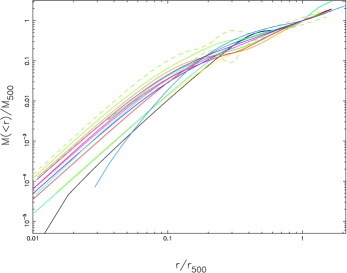
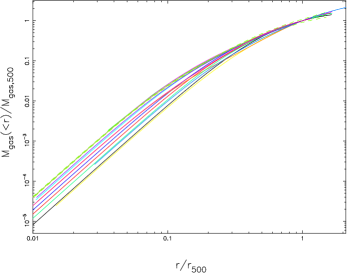
Figure 11: Scaled total mass profiles (left) and gas mass profiles (right) for the REFLEX-DXL sample, with the 1-$\sigma$ error corridor (dashed) displayed for RXCJ0532.9$-$3701. The colours have the same meaning as those in Fig. 4.

The mass profiles were scaled with respect to $M_{\rm 500}$ and $r_{\rm 500}$, respectively (Fig. 11). We found the least scatter at radii above 0.2–0.3 $r_{\rm 500}$. In the inner parts ($<0.2r_{\rm 500}$), the mass profiles vary significantly with the cluster central dynamics (Fig. 11). For the clusters showing cooling cores, the mass distributions are relatively cuspidal, while for the merger clusters, less concentrated mass distributions are observed. The scaled gas mass profiles appear more self-similar than the scaled mass profiles, especially at radii above 0.2–0.3 $r_{\rm 500}$.

4.5 ROSAT and XMM-Newton luminosities

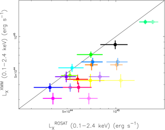
Figure 12: A comparison of the XMM-Newton luminosity and ROSAT luminosity taken from Böhringer et al. (2004). Filled and open circles correspond to the substructure and point-like source subtracted and un-subtracted ROSAT luminosity, respectively. The point-like sources and substructures are detected using the XMM-Newton observations. The colours have the same meaning as those in Fig. 4.

Substructure is often observed in galaxy clusters and the frequency of its occurrence has for example been estimated to be of the order of about $52\pm 7$% (Schuecker et al. 2001). The high resolution XMM-Newton data allow us to identify the substructures and point-like sources better than what was possible with the earlier X-ray telescopes. Subtracting the substructure contribution also from the ROSAT measured cluster luminosity, we found a good agreement between the ROSAT and XMM-Newton luminosity for the REFLEX-DXL clusters (Fig. 12). The XMM-Newton data provide a more reliable and complete detection of substructures and point-like sources. Therefore we make use of this capability to obtain a better approximation to spherical symmetry and dynamical equilibrium of the main, largely relaxed component by excluding the substructures and point-like sources. The properties of the main cluster component are more representative for investigating various scaling relations of regular galaxy clusters, such as the $L$–$T$ relation.

4.6 Scaling relations

To use the temperature/mass function of this unbiased, flux-limited and almost volume-complete sample to constrain cosmological parameters, it is important to calibrate the scaling relations between the X-ray luminosity, temperature and gravitational mass. The scaling relations can generally be parameterized by a power law.

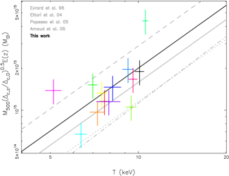
Figure 13: Mass vs. temperature for the REFLEX-DXL sample and the best fit power law (black). The grey lines denote the best fits in Evrard et al. (1996, solid), Ettori et al. (2004, dashed), Popesso et al. (2005, dash-dotted) and Arnaud et al. (2005, dotted). The colours have the same meaning as those in Fig. 4.

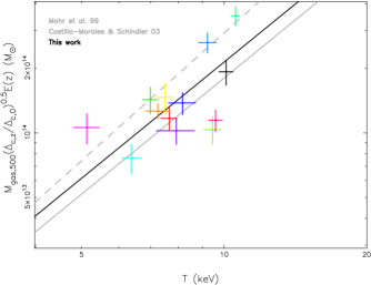
Figure 14: Gas mass vs. cluster temperature and the best fit power law (black). The grey lines denote the best fits in Mohr et al. (1999, dashed) and Castillo-Morales & Schindler (2003, solid). The colours have the same meaning as those in Fig. 4.

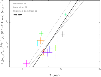
Figure 15: X-ray luminosity in the 0.1–2.4 keV band vs. cluster temperature and the best fit power law (black). The grey lines denote the best fits in Markevitch (1998, solid), Ikebe et al. (2002, dashed), and Reiprich & Böhringer (2002, dash-dotted). The colours have the same meaning as those in Fig. 4.

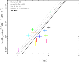
Figure 16: X-ray bolometric luminosity vs. cluster temperature and the best fit power law (black). The grey lines denote the best fits in Markevitch (1998, solid), Arnaud & Evrard (1999, dashed), Xue & Wu (2000, dash-dotted), and Reiprich & Böhringer (2002, dotted). The colours have the same meaning as those in Fig. 4.

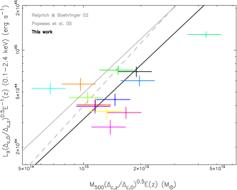
Figure 17: X-ray luminosity in the 0.1–2.4 keV band vs. total mass and the best fit power law (black). The grey lines denote the best fits in Reiprich & Böhringer (2002; dashed) and Popesso et al.(2005, solid). The colours have the same meaning as those in Fig. 4.

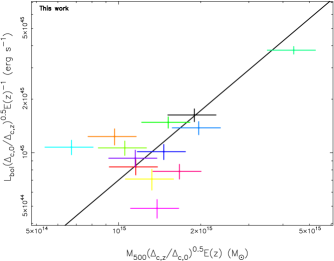
Figure 18: X-ray bolometric luminosity vs. cluster total mass and the best fit power law (black). The colours have the same meaning as those in Fig. 4.

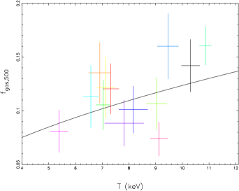
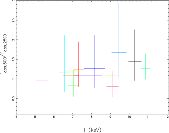
Figure 19: Gas mass fraction $f_{\rm gas,500}$ (left) and Gas mass fraction ratio $f_{\rm gas,500}/f_{\rm gas,2500}$ (right) as a function of cluster temperature. The best fit is $f_{\rm gas,500}\propto T^{0.5\pm 0.3}$. The colours have the same meaning as those in Fig. 4.

The scatter describes the dispersion between the observational data points and the best fit. The scatter in the scaling relation is strongly dependent on the temperature measurement uncertainty. The massive clusters in a narrow temperature range provide an important means to constrain the normalization of the scaling relations such as the $M$–$T$ relation. We collected recently published scaling relations and compared them to the results of this work in Table 6 and Figs. 13–19. The scatter in the scaling relations can partially be explained by variation of the cluster morphology. Comparing the REFLEX-DXL sample to the nearby samples, we found that the evolution of the scaling relations are accounted for by the redshift evolution given in Sect. 4. We obtained an overall agreement with the recent studies of the scaling relations within the observational dispersion. This fits into the general opinion that galaxy clusters are self-similar up to $z\sim 1$ (e.g. Arnaud 2005).

To determine the normalization, the slope of the $M_{500}$–$T$ relation is fixed to 1.5 in the fitting procedure as also used in many published results (e.g. Evrard et al. 1996, Ettori et al. 2004). The $M_{500}$–$T$ relation (Fig. 13) agrees with those in Evrard et al. (1996), Ettori et al. (2004) and Vikhlinin et al (2006). As an unbiased sample, the $M_{500}$–$T$ of the REFLEX-DXL sample shows slightly higher normalization than the local relations found in Finoguenov et al. (2001b) and Popesso et al. (2005), and the local relation derived in Arnaud et al (2005) for relaxed clusters also based on the XMM-Newton temperature profiles. Otherwise, there is no obvious additional evolution of the normalization of the $M$–$T$ relation after the redshift evolution correction. This was also found for the other distant clusters in Maughan et al. (2003) and Ettori et al. (2003).

As shown in Fig. 7, the gas approximately follows DM at radii above $r_{2500}$ for most of the REFLEX-DXL clusters. The gas mass can thus be used as a measure of the total mass. We fixed the slope parameter to 1.8 as also used in Castillo-Morales & Schindler (2003) and Borgani et al. (2004) and fitted the normalization. The $M_{\rm gas,500}$–$T$ relation for the REFLEX-DXL clusters (see Table 6 and Fig. 14) is in good agreement with the relation in Mohr et al. (1999) also using an X-ray flux limited cluster sample. Our result also agrees with the recent result in Castillo-Morales & Schindler (2003). Recent simulations also indicate a strong $M_{\rm gas}$–$T$ scaling relation (e.g. Borgani et al. 2004). The normalization of the $M_{\rm gas,500}$–$T$ relations is slightly higher for the observations than for the simulations (e.g. Borgani et al. 2004).

The X-ray luminosity is a key parameter among the fundamental cluster properties including also mass, temperature, and velocity dispersion. Excluding cooling cores ($\sim 0.1h_{50}^{-1}$ Mpc), Markevitch (1998) reduced the scatter in the $L^{\rm bol}_{\rm X}$–$T$ relation. As listed in Table 3, we list the bolometric X-ray luminosity of the REFLEX-DXL clusters including and excluding the cluster cores, $r<0.1r_{500}$, as is used in many studies (e.g. Markevitch 1998; Zhang 2001). The scatter of the $L$–$T$ relation is reduced by 15% excluding cooling cores. About 8–33% of the luminosity is contributed by the cluster cores ($<0.1r_{500}$) for the REFLEX-DXL clusters. Therefore, the normalization of the $L$–$T$ relation excluding cooling cores is also reduced by 10% for the REFLEX-DXL clusters. As listed in Table 6 and shown in Figs. 15–16, we fixed the slope parameters and fitted the normalizaton for the REFLEX-DXL sample after the redshift evolution correction. Within the observational scatter, the $L^{\rm bol}_{\rm X}$–$T$ relation for the REFLEX-DXL sample (Fig. 16) agrees with the relation in Reiprich & Böhringer (2002) also as an unbiased sample, and the relations in Arnaud & Evrard (1999) and Markevitch (1998). An alternative redshift evolution in the $L$–$T$ relation is described in Kotov & Vikhlinin (2005) yielding $L\propto T^{2.64}(1+z)^{1.8}$. The result here agrees with theirs when the alternative redshift evolution is adopted.

In Fig. 17 and Fig. 18, we show the $L$–$M$ relations (Table 6) of the REFLEX-DXL sample. The slope parameter is fixed to 1.3, as derived in Popesso et al. (2005), in the fitting procedure. The best fit of the normalization of the $L_{\rm X}^{\rm 0.1-2.4keV}$–$M$ relation for the REFLEX-DXL sample agrees with the best fits in Reiprich & Böhringer (2002) and Popesso et al. (2005).

In Fig. 19, we show the gas mass fraction, $f_{\rm gas,500}$, and gas mass fraction ratio, $f_{\rm gas,500}/f_{\rm gas,2500}$, as a function of cluster temperature. We found a weak evidence that the gas mass fraction increases with the cluster temperature, $f_{\rm gas,500}\propto T^{0.5\pm 0.3}$. This agrees with the scaling, $f_{\rm gas,500}\propto T^{0.34\pm 0.22}$, found in Mohr et al (1999). The ratio of the gas mass fractions at larger and smaller radii (e.g. $r_{500}$ and $r_{2500}$) can be used to characterize the extent of gas relative to DM. When this ratio is greater than 1, the gas is more extended than DM (Reiprich 2001). For the REFLEX-DXL clusters, the gas mass ratios (Fig. 19) show that gas is more extended than DM in the cluster inner region but follows DM better in the outer region. Fig. 19 indicates a small trend that the gas is more extended than DM in massive clusters. This indicates that the ICM is less influenced by non-gravitational effects and that the energy input is less important in the outer region for such massive clusters. This is also indicated by simulations (Rowley et al. 2004).

4.7 Intrinsic scatter of the scaling relations

The key to extracting cosmological parameters from the number density of galaxy clusters is a correct understanding of the mass–observable scaling relations and their intrinsic scatter. The scatter of the mass–observable scaling relation describes how well the observable can be used as an estimator of the total mass. The correlative scatter ($\overline{\sigma}_{\rm cor}$) includes the intrinsic scatter ($\overline{\sigma}_{\rm int}$) and observational scatter ($\overline{\sigma}_{\rm obs}$). We investigated the logarithmic intrinsic scatter of the scaling relations, $L$–$T$, $L$–$M$, $M$–$T$, and $M_{\rm gas}$–$T$, of the REFLEX-DXL sample.

The observational scatter $\overline{\sigma}_{\rm obs}$ is the average of the estimated observational uncertainties $\sigma_{\rm obs}$. The correlative scatter $\overline{\sigma}_{\rm cor}$ is the average of the deviation $\sigma_{\rm cor}$ of the observational data points from the best fit of the scaling relation. Assuming that $\sigma_{\rm obs}$ and $\sigma_{\rm cor}$ are not correlated, we apply a Gaussian statistical addition of the two effects to compute the logarithmic intrinsic scatter $\overline{\sigma}_{\rm int}$, the average of $\sigma_{\rm int}=\sqrt{\sigma_{\rm cor}^{2}-\sigma_{\rm obs}^{2}}$ . The reason that we used the average instead of the mean to calculate the scatter lies as following. We investigated the actual distributions of the observational scatter, correlative scatter and logarithmic intrinsic scatter. We found that in most cases the distribution deviates from a Gaussian. Fig. 20 shows for example the distribution of the logarithmic intrinsic scatter of $M_{\rm gas,500}$ for the $M_{\rm gas,500}$–$T$ relation. The merger clusters (e.g. RXCJ0516.7$-$5430 and RXCJ0658.5$-$5556) often fall into the right tail of the histogram. The asymmetry of the histogram is most probably due to the variety of cluster morphologies, e.g. mergers, which can produce significant deviation from the mean. It could also be due to the fact that the REFLEX-DXL sample does not contain enough members to give a pronounced Gaussian statistics. We thus use the average of the histogram to derive the logarithmic intrinsic scatter for the whole sample, which is listed in Table 7 for the scaling relations.

The mass–observable scaling relation which shows the least scatter provides the best prediction for the total mass or gas mass. We find here that the temperature is the best estimator. However, we have to recall that the large uncertainty in the mass estimate comes from the uncertainty in the temperature distribution and therefore part of the reason of the small scatter originates from the fact that the uncertainties are correlated. This is not true for the determination of the gas mass which does hardly depend on the temperature measurement. Therefore the $M_{\rm gas,500}$–$T$ relation, for which we found $\overline{\sigma}_{\rm cor}=0.16$ for $\lg(M_{\rm gas})$ for the REFLEX-DXL sample, is the most remarkably tight correlation.

The scatter of the scaling relations of the REFLEX-DXL sample confirms the recent studies in observations (e.g. Reiprich & Böhringer 2002) and simulations (e.g. Borgani et al. 2004). For example, we obtained the correlative scatter of (0.19,0.20) for ($\lg(L)$,$\lg(M)$) in the $L$–$M_{500}$ relation and confirm the recent studies in observations (e.g. Reiprich & Böhringer 2002) and simulations (e.g. Borgani et al. 2004).

5 Discussion

5.1 Gas profiles in the outskirts

The generally adopted $\beta$-model ($\beta=2/3$) gives $n_{\rm e}\propto r^{-2}$. Mass in-falling becomes significant in the outskirts and thus makes the electron density profile steeper. Vikhlinin et al. (1999) found a mild trend for $\beta$ to increase as a function of cluster temperature, which gives $\beta\sim 0.80$ and $n_{\rm e}\propto r^{-2.4}$ for clusters around 10 keV. Bahcall (1999) also found that the electron number density scales as $n_{\rm e}\propto r^{-2.4}$ at large radii. We confirm their conclusion that $n_{\rm e}\propto r^{-2.42}$ at $r>2^{\prime}$ for the REFLEX-DXL clusters. Due to the gradual change in the slope, one should be cautious to use a single slope double-$\beta$ model which might introduce a systematic error in the cluster mass measurements (as also described e.g. in Horner 2001).

5.2 Validity of the spherical symmetry and hydrostatic equilibrium

The total mass can be underestimated due to the assumption of spherical symmetry for elongated clusters (Castillo-Morales & Schindler 2003). However, a low surface brightness extension is often difficult to subtract correctly because of its less significant boundary relative to the surroundings. In the REFLEX-DXL sample, RXCJ0516.7$-$5430 is such an extreme case. A compression of the photon distribution extends from the cluster center to the north and a low surface brightness extends to $r_{500}$ south of the cluster center. We investigated this cluster and found the global measurements such as $M_{500}$ are insensitive to the inclusion or removal of the region of the low surface brightness extension. The difference of the surface brightness profiles including and excluding the low surface brightness extension is within the 1-$\sigma$ error bar of the surface brightness.

When X-ray images display a pronounced elongated and distorted cluster morphology, the cluster central position cannot be determined unambiguously. For example, RXCJ0014.3$-$3022, RXCJ0516.7$-$5430, RXCJ0528.9$-$3927, RXCJ0658.5$-$5556 and RXCJ1131.9$-$1955 are such cases in the REFLEX-DXL sample. For the case RXCJ0528.9$-$3927, we found that the measurements still agree with each other at the 1-$\sigma$ confidence level using the cluster center of the main component and the center of mass of the two components, respectively.

Clusters showing significant merger features are still dynamically young. These merger features can invalidate the hypothesis of spherical symmetry and hydrostatic equilibrium. For example, RXCJ0658.5$-$5556 is one of the most spectacular merger clusters. We checked the substructure excision method in this work by comparing the results including and excluding the substructure in RXCJ0658.5$-$5556. We found that the global measurements are insensitive to the method excising substructure within the 1-$\sigma$ observational error.

5.3 RXCJ0658.5$-$5556 and the scaling relations

It is worthy to take a closer look, how clusters of particular morphological type affect the scaling relations. We find that the pronounced merger clusters (RXCJ0014.3$-$3022, RXCJ0516.7$-$5430, RXCJ2337.6$+$0016 and RXCJ0658.5$-$5556), which also show an excess in the central entropies and/or large gas mass fractions, introduce a significant broadening of the scatter in the scaling relations. Therefore the scatter has to be considered with caution since it could partially be an artificial effect of the invalidity of hydrostatic equilibrium. A particular case is the extremely hot cluster, RXCJ0658.5$-$5556. For example, excluding RXCJ0658.5$-$5556 the $M_{\rm gas,500}$–$T$ relation provides reduced scatter, $\overline{\sigma}_{\rm cor}=0.11$ and $\overline{\sigma}_{\rm cor}=0.06$ for $M_{\rm gas,500}$ and $T$, respectively.

RXCJ0658.5$-$5556 has a very large weight on the slope of the scaling relations due to its extreme location on the parameter scale. It is also one of the merger systems with large uncertainties of the observational parameters. Therefore we have to be careful with the slope fitting when such merger clusters are involved. As an extreme case, the $S$–$T$ relation of all the REFLEX-DXL clusters gives a slope twice higher than the published empirical slope. In this work, we either fitted the slope parameters excluding merger clusters (e.g. $S$–$T$) or fixed the slope parameters to those in the published papers (e.g. $M$–$T$).

Merger clusters might also affect the determination of the normalization of the scaling relations. Excluding RXCJ0658.5$-$5556, the normalization of the scaling relations of $M_{500}$–$T$, $M_{\rm gas,500}$–$T$, and $L$–$T$ will be reduced by 5%, 5%, and 4%, respectively. RXCJ0658.5$-$5556 lays above the normalized relations by a factor of 1.9,1.5, and 1.1 for $M_{500}$–$T$, $M_{\rm gas,500}$–$T$, and $L$–$T$, respectively.

5.4 Dense core or cool gas

A dense gaseous cluster core, as observed in the CCCs, does not necessarily require a cusp of the DM distribution as described by the extended-NFW model. Alternatively, a sufficiently cooler central temperature also results in a dense core without a cuspy DM profile which is demonstrated as follows. Restricting the analysis to $r<0.5^{\prime}$, we use the pronounced CCC, RXCJ0307.0$-$2840, to illustrate the total mass distribution in the dense and cool gaseous region in the cluster. In general, no cool gas has been observed showing a central temperature lower than half of the mean temperature. We thus assume an extreme temperature drop to 1/3 of the observed temperature of the inner most bin towards the center. Assuming hydrostatic equilibrium, we derived a relatively low mass concentration in the cluster center with the steep central gas density distribution. We can not easily distinguish between the above two cases using the current observations.

5.5 Additional physical processes

We observed a deviation around the self-similar model in the central region in the scaled profiles of the temperature, surface brightness, entropy, total mass and gas mass. This is most probably the effect of different physical processes rather than simply being statistical fluctuations in the measurements (Zhang et al. 2004b, 2005b; Finoguenov et al. 2005). Many studies (e.g. Markevitch et al. 2002; Randall et al. 2002; Finoguenov et al. 2005) show that the X-ray property estimates in the center can be biased by phenomena such as ghost cavities, bubbles, shock and cold fronts, that may somehow invalidate the hydrostatic equilibrium hypothesis and the assumption of homogeneous temperature and density distributions. Complex dynamical interactions with AGN activities have been indicated by the coincidence of CCCs and radio sources (Clarke et al. 2005). M87 shows an example to test the effect of AGN interaction on the X-ray luminosity and also multi-temperature structure (Matsushita et al. 2002).

After subtraction of the effect of measurement uncertainties, the remaining intrinsic scatter in the scaling relations is a signature in variations of cluster structure and ICM processes. This also includes merging clusters as an extreme case (Zhang et al. 2004b). Systematic studies of X-ray mergers have been done in observations using a series of cluster samples (e.g. Schuecker et al. 2001) and simulations (e.g. Schindler & Mueller 1993). Such a detailed study of the REFLEX-DXL clusters using a 2-dimensional approach can be found in Finoguenov et al. (2005).

6 Summary and conclusions

X-ray luminous (massive) clusters are used in a variety of ways to perform both cosmological and astrophysical studies. We selected an unbiased, almost volume-limited sample, the REFLEX-DXL cluster sample, from the REFLEX survey. We performed a systematic analysis to measure the X-ray observables based on high quality XMM-Newton observations, and investigated various X-ray properties and the scaling relations of the REFLEX-DXL cluster sample. We summarize two main conclusions as follows.

(i) An almost self-similar behaviour of the scaled profiles of X-ray properties, such as temperature, surface brightness, entropy, gravitational mass, and gas mass has been found above 0.2–0.3 $r_{500}$ for the REFLEX-DXL sample.

• The average global metallicity is $0.24\pm 0.03Z_{\odot}$ for the whole sample. No significant evolution was found up to $z\sim 0.3$ in the metallicity comparing the REFLEX-DXL sample to the nearby galaxy cluster samples. This agrees with the results in Allen & Fabian (1998), Tozzi et al. (2003), Chen et al. (2003), De Grandi et al. (2004) and Pointecouteau et al. (2004). The results fit into the scenario showing no significant evolution of the iron abundance up to $z\sim 1.1$.

• Based on the XMM-Newton observations, we obtained an average temperature profile of the REFLEX-DXL clusters, which agrees with the previous studies within the observational dispersion. Markevitch et al. (1998) found a steep temperature drop beyond an isothermal center based on ASCA data. De Grandi & Molendi (2002) derived a universal temperature profile which shows a similar decline using BeppoSAX observations. Based on high resolution Chandra observations, Vikhlinin et al. (2005) and Piffaretti et al. (2005) confirmed the previous studies within the observational dispersion, where they found a more pronounced drop outside of 0.2–0.3 $r_{\rm 200}$ in the mean of the universal temperature profile. Additionally, Borgani et al. (2004) reproduced a similar temperature profile in their simulations as found by Vikhlinin et al. (2005). For the REFLEX-DXL sample, we found a universal temperature profile with a peak around 0.2–0.3 $r_{500}$. We observed an almost constant value up to 0.3$r_{500}$ and a very mild decrease to 80% of the peak value at $r>0.3r_{500}$ for the average temperature radial profile of the REFLEX-DXL clusters. However, three clusters (RXCJ0437.1$+$0043, RXCJ0658.5$+$5556, and RXCJ2308.3$+$0211) show temperatures rising with relatively large error bars in their temperature profiles. The average temperature profile declines to 50% of the peak value at radii above $0.3r_{500}$ when these three clusters are excluded. No significant detection of cool gas has been observed showing a central temperature lower than half of the mean temperature.

• We determined the XMM-Newton surface brightness profiles of the REFLEX-DXL clusters up to at least $r_{500}$. We observe steeper profiles at large radii than what is generally obtained for the $\beta$-models with $\beta\sim 2/3$. The surface brightness profiles of most REFLEX-DXL clusters show a flat core populating a broad range of values up to 0.2 $r_{500}$. The total luminosity of the cluster core ($<0.1r_{500}$) accounts for about 8–33% cluster luminosity. For the clusters showing cooling cores, no well-defined constant central density was observed with the XMM-Newton resolution. However, the surface brightness profiles are quite self-similar at $r>0.2r_{500}$ for the REFLEX-DXL sample.

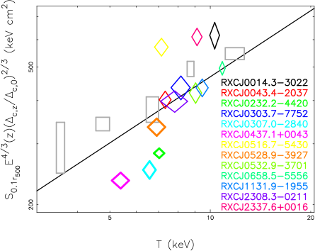
Figure 4: Redshift corrected entropy (diamonds) at $0.1r_{\rm 500}$ vs. $T$ for the REFLEX-DXL clusters. Four clusters showing relatively cool cluster cores are in thick lines. Nearby clusters of Ponman et al. (2003, boxes) are shown for comparison. The solid line denotes the best fits ($S\propto T^{0.63\pm 0.15}$). See the electronic edition of the Journal for a colour version.

• We performed the redshift evolution correction to the entropy profiles at $0.1r_{\rm 500}$ for the REFLEX-DXL clusters and obtained consistency with those for the nearby clusters in Ponman et al. (2003) (see Fig. 4 and Fig. 10) within the observational dispersion. However, four clusters showing relatively cool cores introduce a significant scatter in terms of a lower ($\sim 7\%$) normalization of the $S$–$T$ relation, and three merger clusters introduce some scatter in terms of a higher ($\sim 10\%$) normalization in the $S$–$T$ relation. Excluding these 7 clusters, the REFLEX-DXL sample shows an empirical scaling, $T^{0.63\pm 0.15}$. As shown in Fig. 10, the entropy profiles at $r>0.1r_{500}$ show a similar slope ($S\propto r^{0.99\pm 0.06}$) as observed in Ettori et al. (2002b), $S\propto r^{0.97}$. At the 1-$\sigma$ confidence level, this scaling is shallower than the prediction of the spherical accretion shock model, $S\propto r^{1.1}$ (e.g. Tozzi & Norman 2001; Kay 2004). We found that merger clusters show high central entropies, and the relatively relaxed clusters show lower central entropies. Therefore the central entropy can be used as one means to distinguish the cluster dynamic state. For example, the observational deviation of the ($S$,$T$) data pair from the $S$–$T$ scaling relation for the individual cluster can be used to distinguish the relaxation stage. This may be particularly useful to characterize cluster merging along the line-of-sight, where the merger morphology is less obvious in the projection on the sky.

• We found a self-similar gravitational mass distribution for the REFLEX-DXL sample at radii above 0.2–0.3 $r_{\rm 500}$. The precise gas density and temperature radial profiles provide a detailed diagnostics of the cluster structure and yield reliable determinations of the total mass and gas mass fraction. In the outskirts, the observational density distribution provides an average of $\rho(r)\propto r^{-2.42}$ for the REFLEX-DXL sample.

(ii) The scaling relations of the REFLEX-DXL sample at $z\sim 0.3$ agree with the scaling relations of the nearby samples within the observational dispersion after the redshift evolution correction.

• Since the cluster temperatures of the REFLEX-DXL sample are in a narrow temperature range, the whole sample provides a good means to constrain the normalization of the scaling relations (see Table 6) and to study their intrinsic scatter (see Table 7) at the high mass end.

• The results for the scaling relations of the REFLEX-DXL sample show good agreement compared with previous studies (Table 6). This fits the general opinion (e.g. Maughan et al. 2003; Arnaud 2005; Vikhlinin et al. 2006) that the evolution of galaxy clusters up to $z\sim 1$ is well described by a self-similar model for massive clusters.

• We found that the scatter of the normalization of the scaling relations is very sensitive to the cluster morphology. For example, the scatter of the $L$–$T$ relation is reduced by 15% excluding 4 REFLEX-DXL clusters showing pronounced radiative cooling. Also the normalization of the $L$–$T$ relation excluding those 4 clusters is reduced by 10% for the REFLEX-DXL clusters. We investigated the logarithmic intrinsic scatter of the scaling relations which, for example, gives (0.19,0.20) for ($L$,$M$) in the $L$–$M_{500}$ relation and confirms the recent studies, such as (0.29,0.22) in Reiprich & Böhringer (2002).

Table 1: Properties of the suspicious point-like sources in the cluster center. Column (1): cluster name; Cols. (2,3): sky coordinates in epoch J2000 of the point-like source; Col. (4): index of the best power law fit; Col. (5): X-ray luminosity of the point-like source.

RXCJ	X-ray centroid		Power law	$L_{\rm X}$ (0.1–2.4 keV)
	R.A.	decl.		$10^{44}$ erg s-1
0232.2$-$4420	02 32 18.6	$-$44 20 48.2	$1.77\pm 0.03$	$5.22\pm 0.27$
0437.1$+$0043	04 37 09.8	$+$00 43 48.9	$1.82\pm 0.03$	$3.56\pm 0.18$
0528.9$-$3927	05 28 52.6	$-$39 28 16.8	$1.70\pm 0.05$	$3.20\pm 0.27$
1131.9$-$1955	11 31 54.2	$-$19 55 39.8	$1.75\pm 0.04$	$1.97\pm 0.08$
2308.3$+$0211	23 08 21.6	$-$02 11 29.1	$1.67\pm 0.05$	$2.24\pm 0.12$
2337.6$+$0016	23 37 35.3	$+$00 15 52.1	$1.80\pm 0.06$	$1.02\pm 0.10$

Table 2: Classification of the dynamical state. Column(1): classification; Col.(2): cluster names.

Classification	RXCJ
Single	0307.0$-$2840, 0532.9$-$3701, 2308.3$-$0211
Primary with small secondary	0232.2$-$4420, 0303.7$-$7752
Elliptical	0043.4$-$2037, 0437.1$+$0043, 0516.7$-$5430, 1131.9$-$1955
Offset center	0014.3$-$3022, 0528.9$-$3927, 0658.5$-$5556, 2337.6$+$0016
Complex	2011.3$-$5725

Classifications see Jones & Forman (1992).

Table 3: Primary parameters. Column (1): cluster name; Col. (2): optical redshift (Böhringer et al. 2004); Cols. (3,4): sky coordinates in epoch J2000 of the cluster center; Col. (5): hydrogen column density in units of $10^{20}{\rm cm}^{-2}$ (Dickey & Lockman 1990); Col. (6):X-ray measured redshift; Col. (7): truncation radius corresponding to a $S/N$ of 3 of the observational surface brightness profile; Cols. (8,9): cluster global temperature and global metallicity in the 0.1–0.5 $r_{500}$ region; Cols. (10,11): bolometric luminosity including and excluding cluster core ($<0.1r_{500}$).

RXCJ	$z_{\rm opt}$	X-ray centroid		$N_{\rm H}$	$z_{\rm X-ray}$	$r_{\rm t}$	$T$	$Z$	$L_{\rm bol}^{\rm incc}$	$L_{\rm bol}^{\rm excc}$
		R.A.	decl.	$10^{20}$ cm-2		arcmin	keV	$Z_{\odot}$	$10^{45}$ erg s-1
0014.3$-$3022	0.3066	00 14 18.6	$-30$ 23 15.4	1.60	$0.28\pm 0.01$	7.61	$10.1\pm 0.3$	$0.17\pm 0.05$	$2.12\pm 0.17$	$1.91\pm 0.16$
0043.4$-$2037	0.2924	00 43 24.5	$-20$ 37 31.2	1.54	$0.28\pm 0.01$	7.02	$7.7\pm 0.3$	$0.11\pm 0.06$	$1.07\pm 0.11$	$0.89\pm 0.09$
0232.2$-$4420	0.2836	02 32 18.8	$-44$ 20 51.9	2.49	$0.27\pm 0.01$	6.81	$7.0\pm 0.3$	$0.10\pm 0.05$	$1.89\pm 0.14$	$1.27\pm 0.11$
0303.7$-$7752	0.2742	03 03 47.2	$-77$ 52 39.0	8.73	$0.26\pm 0.01$	7.53	$8.2\pm 0.5$	$0.32\pm 0.08$	$1.29\pm 0.13$	$1.04\pm 0.11$
0307.0$-$2840	0.2578	03 07 02.2	$-28$ 39 55.2	1.36	$0.24\pm 0.01$	4.70	$6.4\pm 0.3$	$0.13\pm 0.06$	$1.34\pm 0.13$	$1.00\pm 0.10$
0437.1$+$0043	0.2842	04 37 09.5	$+00$ 43 54.5	8.68	$0.31\pm 0.02$	7.73	$5.1\pm 0.3$	$0.30\pm 0.11$	$0.62\pm 0.07$	$0.42\pm 0.06$
0516.7$-$5430	0.2943	05 16 35.2	$-54$ 30 36.8	6.86	$0.28\pm 0.01$	6.39	$7.5\pm 0.3$	$0.16\pm 0.07$	$0.92\pm 0.12$	$0.84\pm 0.11$
0528.9$-$3927	0.2839	05 28 52.5	$-39$ 28 16.7	2.12	$0.26\pm 0.02$	5.80	$7.2\pm 0.4$	$0.42\pm 0.08$	$1.58\pm 0.16$	$1.25\pm 0.13$
0532.9$-$3701	0.2747	05 32 55.9	$-37$ 01 34.5	2.90	$0.27\pm 0.01$	7.01	$9.5\pm 0.4$	$0.32\pm 0.07$	$1.35\pm 0.12$	$0.95\pm 0.10$
0658.5$-$5556	0.2965	06 58 30.2	$-55$ 56 33.7	6.53	$0.29\pm 0.01$	8.88	$10.6\pm 0.2$	$0.26\pm 0.03$	$4.87\pm 0.24$	$4.21\pm 0.21$
1131.9$-$1955	0.3075	11 31 54.7	$-19$ 55 40.5	4.50	$0.33\pm 0.03$	9.00	$9.2\pm 0.4$	$0.27\pm 0.05$	$1.80\pm 0.15$	$1.58\pm 0.14$
2308.3$-$0211	0.2966	23 08 22.3	$-02$ 11 32.1	4.45	$0.27\pm 0.02$	7.31	$7.9\pm 0.7$	$0.31\pm 0.14$	$1.20\pm 0.13$	$0.88\pm 0.11$
2337.6$+$0016	0.2753	23 37 37.8	$+00$ 16 15.5	3.82	$0.27\pm 0.01$	7.27	$9.6\pm 0.3$	$0.25\pm 0.06$	$1.00\pm 0.09$	$0.79\pm 0.08$

Table 4: Deduced properties of the REFLEX-DXL clusters. Column (1): cluster name; Col. (2): central electron number density; Col. (3): central entropy; Cols. (4,5): cooling time and cooling radius; Col. (6): $r_{500}$; Cols. (7–9): gas mass, total mass, and gas mass fraction at $r_{500}$.

RXCJ	$n_{e0}$	$S_{0}$	$t_{\rm c}$	$r_{\rm cool}$	$r_{500}$	$M_{\rm gas,500}$	$M_{500}$	$f_{\rm gas,500}$
($10^{-3}$ cm-3)		(keV cm2)	(Gyr)	(Mpc)	(Mpc)	($10^{14}M_{\odot}$)	($10^{14}M_{\odot}$)
0014.3$-$3022	$3.7\pm 0.2$	$421\pm 37$	$14.1\pm 0.6$	$0.00$	$1.24$	$1.0\pm 0.2$	$7.4\pm 2.9$	$0.142\pm 0.024$
0043.4$-$2037	$5.8\pm 0.4$	$293\pm 17$	$10.2\pm 0.3$	$0.12$	$1.08$	$0.6\pm 0.1$	$4.8\pm 1.8$	$0.120\pm 0.023$
0232.2$-$4420	$14.0\pm 0.1$	$279\pm 10$	$10.3\pm 0.2$	$0.18$	$1.30$	$0.9\pm 0.2$	$8.4\pm 2.4$	$0.105\pm 0.023$
0303.7$-$7752	$6.0\pm 0.4$	$311\pm 24$	$10.3\pm 0.4$	$0.12$	$1.27$	$0.8\pm 0.1$	$7.7\pm 2.3$	$0.101\pm 0.022$
0307.0$-$2840	$10.2\pm 0.3$	$265\pm 16$	$10.5\pm 0.3$	$0.17$	$1.14$	$0.6\pm 0.1$	$5.5\pm 1.1$	$0.113\pm 0.029$
0437.1$+$0043	$10.1\pm 0.4$	$223\pm 14$	$10.2\pm 0.3$	$0.16$	$1.17$	$0.5\pm 0.1$	$6.1\pm 2.2$	$0.081\pm 0.020$
0516.7$-$5430	$2.9\pm 0.2$	$403\pm 24$	$16.7\pm 0.4$	$0.00$	$1.19$	$0.8\pm 0.2$	$6.4\pm 2.1$	$0.122\pm 0.029$
0528.9$-$3927	$10.6\pm 0.4$	$280\pm 16$	$10.3\pm 0.3$	$0.14$	$1.19$	$0.9\pm 0.1$	$6.4\pm 1.5$	$0.135\pm 0.028$
0532.9$-$3701	$13.3\pm 0.5$	$337\pm 23$	$10.4\pm 0.3$	$0.14$	$1.13$	$0.6\pm 0.1$	$5.4\pm 1.7$	$0.107\pm 0.024$
0658.5$-$5556	$6.1\pm 0.2$	$354\pm 16$	$10.1\pm 0.2$	$0.15$	$1.42$	$1.8\pm 0.3$	$11.0\pm 6.8$	$0.161\pm 0.018$
1131.9$-$1955	$5.8\pm 0.3$	$307\pm 18$	$10.0\pm 0.3$	$0.11$	$1.10$	$0.8\pm 0.2$	$5.2\pm 3.0$	$0.160\pm 0.030$
2308.3$-$0211	$9.2\pm 0.3$	$296\pm 22$	$10.1\pm 0.3$	$0.14$	$1.24$	$0.7\pm 0.1$	$7.4\pm 1.8$	$0.089\pm 0.022$
2337.6$+$0016	$5.7\pm 0.3$	$372\pm 21$	$12.3\pm 0.3$	$0.00$	$1.43$	$0.8\pm 0.1$	$10.9\pm 2.6$	$0.074\pm 0.016$
Mean	—	—	—	—	—	—	—	$0.116\pm 0.007$

Table 5: Parameters of the extended-NFW model fits of the REFLEX-DXL clusters. Column (1): cluster name; Cols. (2,3): characteristic density and scale of the halo; Cols. (4): slope parameter; Col. (5): $\chi^{2}$ and its degree of freedom (d.o.f.); Col. (6): concentration parameter at $r_{500}$.

RXCJ	$\rho_{\rm s}$	$r_{\rm s}$	$\alpha$	$\chi^{2}/$d.o.f.	$c_{500}$
	($M_{\odot}$ Mpc-3)	(Mpc)
0014.3$-$3022	$(2.7\pm 0.3)\times 10^{4}$	$0.16\pm 0.01$	$-1.69$	90.0/157	$7.5\pm 1.5$
0043.4$-$2037	$(1.8\pm 0.2)\times 10^{4}$	$0.15\pm 0.01$	$-0.56$	30.9/115	$7.4\pm 1.5$
0232.2$-$4420	$(1.3\pm 0.7)\times 10^{2}$	$1.13\pm 0.74$	$1.28$	65.7/124	$1.2\pm 0.4$
0303.7$-$7752	$(8.8\pm 0.6)\times 10^{3}$	$0.22\pm 0.01$	$-0.17$	18.0/143	$5.7\pm 1.2$
0307.0$-$2840	$(3.7\pm 0.2)\times 10^{4}$	$0.11\pm 0.01$	$-0.87$	3.8/82	$10.7\pm 2.2$
0437.1$+$0043	$(6.2\pm 0.7)\times 10^{3}$	$0.23\pm 0.01$	$0.08$	34.8/97	$5.1\pm 1.1$
0516.7$-$5430	$(2.5\pm 0.2)\times 10^{3}$	$0.38\pm 0.02$	$-0.09$	21.4/131	$3.1\pm 0.6$
0528.9$-$3927	$(4.6\pm 2.6)\times 10^{4}$	$0.08\pm 0.02$	$-0.51$	113.8/56	$14.6\pm 4.4$
0532.9$-$3701	$(6.9\pm 1.1)\times 10^{4}$	$0.80\pm 0.01$	$-0.65$	39.7/118	$14.2\pm 3.0$
0658.5$-$5556	$(4.0\pm 0.6)\times 10^{3}$	$0.43\pm 0.03$	$-0.27$	333.6/240	$3.3\pm 0.7$
1131.9$-$1955	$(1.2\pm 0.3)\times 10^{6}$	$0.04\pm 0.01$	$-7.71$	49.9/128	$30.0\pm 6.6$
2011.3$-$5725	$(4.3\pm 4.1)\times 10^{4}$	$0.07\pm 0.03$	$-0.44$	7.0/8	$4.2\pm 0.5$
2308.3$-$0211	$(2.4\pm 0.3)\times 10^{4}$	$0.13\pm 0.01$	$-0.31$	9.4/58	$9.7\pm 2.0$
2337.6$+$0016	$(6.8\pm 1.9)\times 10^{3}$	$0.23\pm 0.03$	$0.12$	82.1/91	$6.3\pm 1.5$

Table 6: Power law, $Y=Y_{0}\;X^{\gamma}$, parameterized scaling relations in this work and in literature.

$Y$	$X$	$Y_{0}$	$\gamma$	Reference
$\frac{M_{500}}{M_{\odot}}\;E(z)\;(\Delta_{c,z}/\Delta_{c,0})^{0.5}$	$\frac{T}{\rm keV}$	$10^{13.85}h_{50}^{-1}$	1.5 (fixed)	Evrard et al. 96
		$10^{13.63^{+0.08}_{-0.07}}h_{50}^{-1}$	$1.48^{+0.10}_{-0.12}$	Finoguenov et al. 01b
		$10^{13.96\pm 0.02}h_{70}^{-1}$	1.5 (fixed)	Ettori et al. 04
		$10^{13.46\pm 0.02}h_{70}^{-1}$	$1.59\pm 0.05$	Popesso et al. 05
		$10^{13.57\pm 0.02}h_{70}^{-1}$	$1.49\pm 0.15$	Arnaud et al. 05
		$10^{13.80\pm 0.04}h_{70}^{-1}$	1.5 (fixed)	This work
$\frac{M_{\rm gas,500}}{M_{\odot}}\;E(z)\;(\Delta_{c,z}/\Delta_{c,0})^{0.5}$	$\frac{T}{\rm keV}$	$10^{12.63\pm 0.03}h_{50}^{-1}$	$1.98\pm 0.18$	Mohr et al. 99
		$10^{12.60}h_{50}^{-1}$	$1.80\pm 0.16$	Castillo-Morales & Schindler 03
		$10^{12.53\pm 0.04}h_{70}^{-1}$	1.8 (fixed)	This work
$\frac{L_{\rm X}^{\rm 0.1-2.4keV}}{\rm erg\;s^{-1}}\;E(z)^{-1}\;(\Delta_{c,z}/\Delta_{c,0})^{-0.5}$	$\frac{T}{\rm keV}$	$10^{42.52\pm 0.04}h_{100}^{-1}$	$2.10\pm 0.24$	Markevitch 98
		$10^{42.79\pm 0.09}h_{50}^{-1}$	$2.60\pm 0.13$	Reiprich & Böhringer 02
		$10^{42.19\pm 0.29}h_{50}^{-1}$	$2.44\pm 0.39$	Ikebe et al. 02
		$10^{42.37\pm 0.06}h_{70}^{-1}$	2.60 (fixed)	This work
$\frac{L_{\rm bol}}{\rm erg\;s^{-1}}\;E(z)^{-1}\;(\Delta_{c,z}/\Delta_{c,0})^{-0.5}$	$\frac{T}{\rm keV}$	$10^{42.43\pm 0.04}h_{100}^{-1}$	$2.64\pm 0.27$	Markevitch 98
		$10^{42.82\pm 0.03}h_{50}^{-1}$	$2.88\pm 0.15$	Arnaud & Evrard 99
		$10^{42.97\pm 0.07}h_{50}^{-1}$	$2.79\pm 0.08$	Xue & Wu 00
		$10^{42.85\pm 0.09}h_{50}^{-1}$	$2.98\pm 0.12$	Reiprich & Böhringer 02
		$10^{42.38\pm 0.06}h_{70}^{-1}$	2.98 (fixed)	This work
$\frac{L_{\rm X}^{\rm 0.1-2.4keV}}{\rm erg\;s^{-1}}\;E(z)^{-1}\;(\Delta_{c,z}/\Delta_{c,0})^{-0.5}$	$\frac{M_{500}}{M_{\odot}}\;E(z)\;(\Delta_{c,z}/\Delta_{c,0})^{0.5}$	$10^{22.455\pm 1.298}h_{50}^{-1}$	$1.504\pm 0.089$	Reiprich & Böhringer 02
		$10^{25.19\pm 0.10}h_{70}^{-1}$	$1.30\pm 0.12$	Popesso et al. 05
		$10^{25.00\pm 0.06}h_{70}^{-1}$	1.3 (fixed)	This work
$\frac{L_{\rm bol}}{\rm erg\;s^{-1}}\;E(z)^{-1}\;(\Delta_{c,z}/\Delta_{c,0})^{-0.5}$	$\frac{M_{500}}{M_{\odot}}\;E(z)\;(\Delta_{c,z}/\Delta_{c,0})^{0.5}$	$10^{25.35\pm 0.06}h_{70}^{-1}$	1.3 (fixed)	This work
$f_{\rm gas,500}$	$\frac{T}{\rm keV}$	$0.035\pm 0.030h^{-3/2}_{70}$	$0.5\pm 0.3$	This work

Table 7: Logarithmic intrinsic scatter measured for the scaling relations. Column(1): scaling relation; Col.(2): variable; Cols.(3,4): logarithmic intrinsic scatter and correlative scatter.

Relation	Variable	$\overline{\sigma}_{\rm int}$	$\overline{\sigma}_{\rm cor}$
$M_{500}$–$T$	$\lg(M_{500})$	0.17	0.20
	$\lg(T)$	0.09	0.10
$M_{\rm gas,500}$–$T$	$\lg(M_{\rm gas,500})$	0.14	0.16
	$\lg(T)$	0.07	0.08
$L_{X}^{\rm 0.1-2.4keV}$–$T$	$\lg(L_{X}^{\rm 0.1-2.4keV})$	0.16	0.17
	$\lg(T)$	0.06	0.07
$L_{X}^{\rm 0.1-2.4keV}$–$M_{500}$	$\lg(L_{X}^{\rm 0.1-2.4keV})$	0.19	0.20
	$\lg(M_{500})$	0.16	0.19
$L_{\rm bol}$–$T$	$\lg(L_{\rm bol}$	0.16	0.17
	$\lg(T)$	0.06	0.07
$L_{\rm bol}$–$M_{500}$	$\lg(L_{\rm bol}$	0.18	0.19
	$\lg(M_{500})$	0.17	0.20

Figure 2: De-projected temperature profiles of the REFLEX-DXL clusters. The temperature profiles are approximated by the parameterization $T(r)=T_{3}\exp[-(r-T_{1})^{2}/T_{2}]+T_{6}(1+r^{2}/T_{4}^{2})^{-T_{5}}+T_{7}$ crossing all the data points (solid). The 1-$\sigma$ confidence intervals are approximated by $T(r)[1\pm(T_{8}+T_{9}r)]$ (dashed). The vertical line denotes $0.1r_{500}$.

Figure 3: Surface brightness profiles of the REFLEX-DXL clusters and their best fits. Residuals scaled by the data uncertainties are plotted in the upper part of the diagrams.

Figure 5: Measured mass profiles of the REFLEX-DXL clusters and their best fits by the extended-NFW models. Residuals scaled by the data uncertainties are plotted in the upper part of the diagrams.

Figure 20: Histogram of the intrinsic scatter for $\lg(M_{\rm gas,500})$ of the $M_{\rm gas,500}$–$T$ relation for the REFLEX-DXL clusters.