Interferometric Parallax:
A Method for Measurement of Astronomical Distances

Abstract

We show that distances of objects at cosmological distances can be measured directly using interferometry. Our approach to interferometric parallax comes from analysis of 4-point amplitude and intensity correlations that can be generated from pairs of well-separated detectors. The baseline required to measure cosmological distances of Gigaparsec order are within the reach of the next generation of space-borne detectors. The semi-classical interpretation of intensity correlations uses a notion of a single photon taking two paths simultaneously. Semi-classically a single photon can simultaneously enter four detectors separated by an astronomical unit, developing correlations feasible to measure with current technology.

There is no more important problem in astronomy than resolving the third dimension of source distances. The crisis of dark energy and dark matter in cosmology hinges on distance measurements. Estimates using red shifts or Type 1a supernova sources are weakened by model dependence of the cosmology and assumptions on the evolution of distant sources. Here we show that direct measurements of cosmologically distance objects can be made from the analysis of correlations of detectors separated on the scale of the solar system. Correlations of amplitudes (first order coherence) are used in Michelson’s interferometer and radio telescopes. The breakthrough of Hanbury-Brown and Twiss ($HBT$)HBT demonstrated 2-point correlations of intensity (second order coherence) developed by counting photon fluxes in separated detectors. Higher order correlations have been proposed earlier for reconstructing the phase of the coherence function phase and to improve the sensitivity sensitivity in intensity correlations. We show that 4-point amplitude and intensity correlations contain further information on the distance to the sources. The baseline required to measure cosmological distances of Gigaparsec order are within the reach of the next generation of space-borne detectors. Measuring source distances of Megaparsec order appears feasible now.

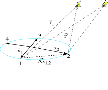
Figure 1: Four detectors are positioned so that the relative position vector $\Delta\vec{x}_{12}$ between one pair is approximately the same as between another pair $\Delta\vec{x}_{34}$, with a net translation $\vec{X}$ between the pairs.

Let $\vec{x}_{i}$ be the position vectors of the $i$th detector relative to the origin (Fig. 1). Consider a point source at $\vec{r}=\hat{r}r$ relative to the origin, also located at position $\vec{r}_{J}$ relative to each detector:

$$\vec{r}_{J}=\vec{r}-\vec{x}_{J}.$$

Calculate the distance from the $J$th detector to the source to order $1/r$:

$$r_{J}=r-\hat{r}\cdot\vec{x}_{J}+{x_{J}^{i}\delta_{T}^{ij}x_{J}^{j}\over 2r}+O(1/r^{2}),$$ (1)

where $\delta_{T}^{ij}(r)=\delta^{ij}-\hat{r}^{i}\hat{r}^{j}.$ Here upper indices denote vector components. The third term depends on the distance $r$ and will be responsible for probing it via interferometric parallax. The frequency-domain Green function for propagation from source to receiver is expanded

$$G_{x_{J}\vec{r}} = {e^{ik|\vec{r}-\vec{x}_{{}^{\prime}J}|}\over|\vec{r}-\vec{x}_{J}|}\sim{e^{ikr}\over r}e^{-ik\hat{r}\cdot\vec{x}_{J}}e^{ik{x_{J}^{i}\delta_{T}^{ij}x_{J}^{j}/(2r})}$$

where $k$ is the wave number. We drop the $e^{ikr}/r$ prefactor which cancels out in calculations. The formula extends trivially to two distinct sources, $S$ and $S^{\prime}$, for which primed symbols such as $\vec{r}^{\prime}=\hat{r}^{\prime}r^{\prime}$ take the obvious meaning.

Concentrate for a moment on two detectors 1, 2. Standard analysis of the interferometric correlation treats the electric field $\vec{E}$ as a random variable, described by convolution of the Green function with correlations of the source. Then the amplitude correlation for a single polarization between the two receivers can be expressed as,

$$<E_{1}E_{2}^{*}>=e^{-ik\psi}\Bigg{[}{I_{0}\over r^{2}}+{I_{0}^{\prime}\over r^{\prime 2}}e^{-i\phi_{12}^{(0)}-i\phi_{12}^{parallax}}\Bigg{]}$$ (2)

where $\vec{E}_{0}$ is the field of one source, $I_{0}=<E_{0}E_{0}^{*}>$, and so on for primed variables. Here

$$\phi_{12}^{(0)} = -k(\vec{x}_{1}-\vec{x}_{2})\cdot(\hat{r}-\hat{r}^{\prime});$$

$$\phi_{12}^{parallax} = k(\vec{x}_{1}^{i}\vec{x}_{1}^{j}-\vec{x}_{2}^{i}\vec{x}_{2}^{j})\left({\delta_{T}(r)^{ij}\over 2r}-{\delta_{T}(r^{\prime})^{ij}\over 2r^{\prime}}\right).$$ (3)

The overall phase $\psi=\hat{r}\cdot(\vec{x}_{1}-\vec{x}_{2})-(x_{1}^{i}x_{1}^{j}-x_{2}^{i}x_{2}^{j})\delta_{T}^{ij}/2r$. The overall phase cancels in a determination of the absolute value of the correlation. In eq. 2, the source-detector distances are consistently replaced by $r$ and $r^{\prime}$ everywhere except in the phases.

The intensity-intensity correlations, $<I_{1}I_{2}>=<|E(\vec{x}_{1})|^{2}|E(\vec{x}_{2})|^{2}>$ between receivers 1 and 2 for classical light are found to be,

$$<I_{1}I_{2}> = \left({I_{0}\over r^{2}}+{I^{\prime}_{0}\over r^{\prime 2}}\right)^{2}+{I_{0}^{2}\over r^{4}}+{{I^{\prime}}_{0}^{2}\over r^{{}^{\prime}4}}$$ (4)

$$+ {2I_{0}I^{\prime}_{0}}\Re(\,G_{1r}G^{*}_{1r^{\prime}}G_{2r^{\prime}}G_{2r}^{*}\,)$$

$$= \left({I_{0}\over r^{2}}+{I^{\prime}_{0}\over r^{\prime 2}}\right)^{2}+{I_{0}^{2}\over r^{4}}+{{I^{\prime}}_{0}^{2}\over r^{{}^{\prime}4}}+$$

$$+ {2I_{0}I^{\prime}_{0}\over r^{2}r^{\prime 2}}\Re\left(e^{i\phi_{12}^{(0)}+i\phi_{12}^{parallax}}\right).$$

Here $\Re$ denotes the real part. A quantum mechanical calculation gives a similar result, and incorporates photon bunching. We see that $\phi^{parallax}$ appears in both amplitude and intensity correlations. Intensity correlations can be used at optical frequencies by simply counting photons, and have certain advantages in automatically canceling the overall phase $\psi$.

The first phase $\phi^{(0)}$ has been used extensively for angular position measurements. Notice that this phase is translationally invariant - it depends only on the relative position vector of the two detectors. The scale $\Delta x_{12}$ is conjugate to a difference of wave numbers, not the radiation wavelength. Our focus is on the second phase $\phi_{12}^{parallax}$. Consulting Fig. 1, let detectors 1 and 2 be located at average position $\vec{X}$ and separated by $\Delta\vec{x}_{12}$: $\vec{x}_{1}=\vec{X}-\Delta\vec{x}_{12}/2,\,\vec{x}_{2}=\vec{X}+\Delta\vec{x}_{12}/2.$ By substitution the second phase is

$$\phi_{12}^{parallax}=-k\Delta\vec{x}_{12}\cdot\left({\delta_{T}(r)\over r}-{\delta_{T}(r^{\prime})\over r^{\prime}}\right)\cdot\vec{X}.$$ (5)

This phase will change with $\vec{X}$ even if $\Delta\vec{x}_{12}$ is fixed. The explanation of course is parallax sensed via curved wave fronts. A measurement of the correlation’s dependence on translating a fixed detector pair in $\vec{X}$ can probe the distance dependence on $1/r$ and $1/r^{\prime}$.

We emphasize that interferometric parallax is qualitatively different from standard trigonometric parallax long used in astronomy. In trigonometric parallax the distance is estimated by a precise measurement of the angular position of the source from two different locations. For interferometric parallax a precise measurement of the angular position is not required, and dependence on the angular position is weak. Strictly speaking, the individual sources need not be resolved. Sensitivity exists in selecting source for the measurement, and excluding background.

We now discuss finite source size effects. The basic two point amplitude correlation for an incoherent source component located at $\vec{r}_{i}+\vec{y}$ is

$$<E(\vec{x}_{1})E^{*}(\vec{x}_{2})> = \int d^{2}y<E_{0}(\vec{y})E_{0}^{*}(\vec{y})>$$ (6)

$$\times {e^{ik[|\vec{r}_{1}+\vec{y}|-|\vec{r}_{2}+\vec{y}|}\over|\vec{r}_{1}+\vec{y}||\vec{r}_{2}+\vec{y}|},$$

$$= e^{ik(r_{1}-r_{2})}{\cal I}.$$

Here we have expanded the argument of the exponential integrand as

$$|\vec{r}_{1}+\vec{y}|-|\vec{r}_{2}+\vec{y}|=r_{1}-r_{2}+\hat{r}_{1}\cdot\vec{y}-\hat{r}_{2}\cdot\vec{y}$$

$$-(\vec{y}\cdot\hat{r}_{1})^{2}/2r+(\vec{y}\cdot\hat{r}_{2})^{2}/2r.$$

By inspection the last two terms only contribute at order $1/r^{2}$. Let $a$ be the effective transverse size of the source. All terms involved in ${\cal I}$ are functions of the angular size of the source $a/r$, and ${\cal I}$ is negligibly small if $a/r>>1/(k\Delta x)$. As long as $\Delta x\lesssim a/(kr)$ the corrections due to finite size can be absorbed into the overall factors $I_{0}$, $I_{0}^{\prime}$ etc. in Eq. 2, and a source appears to be a point. This reproduces the usual planar source criterionoptics that an observable signal requires baselines smaller than the coherence zone of each source. All higher order correlations for two sources can be expressed as products of such two point amplitude correlations of individual sources, justifying the point source approximation.

Orders of Magnitude: For wavelength $\lambda$ and typical source angular separation $\Delta\theta$ we have $\phi_{12}^{(0)}\sim{\Delta\theta/(\lambda/\Delta x_{12})}$ and $\phi_{12}^{parallax}\sim{X/r/(\lambda/\Delta x_{12})}.$ We recognize $\lambda/\Delta x_{12}$ as the lower limit on angular resolution from optics. Similarly, the parallax phase is of order one if the baseline of translation $X$ could be resolved by an instrument of aperture $\Delta x$ looking from distance $r$. Using the lower limit of the single-source coherence $k\Delta x\lesssim r/a$ gives $\phi_{12}^{parallax}\sim(X/a)(1-r/r^{\prime}).$ For $\phi_{12}^{parallax}\sim 1$ and comparable $r,\,r^{\prime}$ the source-size should match the translational scale. Of course the coherence zone criteria do not require literally small sources, but represent the existence of Fourier modes (structure) in the regime of size indicated. Setting $\phi_{12}^{parallax}\sim 1$ yields the distance scale that can be observed:

$$r\lesssim 1\,Gpc\,{X\over AU}{\Delta x\over AU}{1{\rm mm}\over\lambda}.$$ (7)

Although phases can often be measured with exquisite accuracy, we will continue assuming $\phi^{parallax}\sim 1$ for our estimates. Consider detectors separated by $10^{4}$ km, a near Earth orbit, and translating over $X\sim 1AU$ in a period of a year. Numerically

$$\phi_{12}^{(0)}\sim 10^{5}{\Delta\theta\over arcsec}{{\rm 1mm}\over\lambda}{\Delta x_{12}\over 10^{4}km};$$

$$\phi_{12}^{parallax}\sim 10^{-4}\,{X\over AU}{1{\rm Gpc}\over r}{{\rm 1mm}\over\lambda}{\Delta x_{12}\over 10^{4}km}.$$ (8)

Baselines of order $10^{4}$ km at $cm$ wavelengths have been demonstrated by current technology. For Gpc distances, one needs to measure a relatively small phase or push the limits of baselines to much larger than $10^{4}$ Km and/or wavelength to the sub-mm range. This may be possible due to the huge range of possibilities for $\Delta\theta$. Quasar sources are believed to have physical sizes extending to the range of 1 AU, whereby $\Delta\theta\sim 10^{-9}\,arcsec$ at distances of $Gpc$ order. The maximum coherence zone for such sources $\Delta x\sim\lambda r/a\sim 10^{11}m\,(\lambda/mm)(r/Gpc)(AU/a)$ are compatible with baselines of order AU. Black hole and GRB sources are of course even smaller, with correspondingly larger coherence zones. It might also be possible to measure gravitationally lensed single objects, exploiting two path lengths $r$, $r^{\prime}$. In principle measurement of $\phi_{12}^{parallax}$ of order unity can measure distances to Gpc order provided suitable sources can be exploited.

The ratio $\phi^{(0)}/\phi^{parallax}\sim 10^{8}$ for a typical value of $\Delta\theta\sim 0.1arcsec$ assuming Gpc distance. There are reasons to expect high control over $\phi^{(0)}$ by technological means. However for the rest of the paper we consider “worst case” scenarios, in which control of $\phi^{(0)}$ is less than ideal. There happens to be a practical strategy to null out the effects of the rapidly varying phase. To control the effects of $\phi^{(0)}$ we can (in effect) measure it twice, using another pair of detectors 3, 4, separated by the “same” offset: $\Delta\vec{x}_{34}=\Delta\vec{x}_{12}+\vec{\eta}\ .$ It is clear that $\vec{\eta}<<\Delta\vec{x}_{12}$ can be made relatively small with great precision. We consider the product of $<I_{1}I_{2}><I_{3}I_{4}>$, which is one of the terms in the 4-point intensity correlation. Denoting the overall normalizations by $N_{1}$ and $N_{2}$ we write

$$<I_{1}I_{2}>=N_{1}+N_{2}\cos(A+B);$$

$$<I_{3}I_{4}>=N^{\prime}_{1}+N^{\prime}_{2}\cos(A^{\prime}+B^{\prime}),$$

where $A=\phi_{12}^{(0)}$, $B=\phi_{12}^{parallax}$, with the primes switching 12 $\rightarrow 34$. In an experiment where $A>>B$ and $\Delta x_{12}\cdot(\hat{r}-\hat{r}^{\prime})$ varies rapidly the products with an odd number of cosines will average to zero. The average here (symbol $<<\,>>$) might occur over running time in which drifts of the detector position values cause $\phi^{(0)}$ to vary. Another cause of variation lies in small ranges in $\omega$ differing between the detectors, and there are no doubt other possible causes. The term with two cosines gives

$$<<\,\cos(A+B)\cos(A^{\prime}+B^{\prime})\,>>=$$

$$<<\,\cos A\cos A^{\prime}\,>>\cos B\cos B^{\prime}$$

$$+<<\,\sin A\sin A^{\prime}\,>>\sin B\sin B^{\prime}.$$

The only non-zero data will come from $<<\,\cos A\cos A^{\prime}\,>>=<<\,\sin A\sin A^{\prime}\,>>=1/2$, namely those regimes when the rapidly varying terms coincide.

Collecting the terms gives

$$<I_{1}I_{2}><I_{3}I_{4}>=N_{1}N^{\prime}_{1}+N_{2}N^{\prime}_{2}\cos(B-B^{\prime})$$

$$=N_{1}N_{1}^{\prime}+N_{2}N_{2}^{\prime}\cos(\phi_{12}^{parallax}-\phi_{34}^{parallax}).$$ (9)

Since the net translation of the 3-4 receiver pair is independent of the 12 pair, it is straightforward to arrange for the surviving slow oscillation to produce a net signal. A simple configuration (Fig. 1) puts $\Delta x_{12}=\Delta x_{34}=\Delta x,\,\vec{x}_{3}=-\vec{X}-\Delta x/2,\,\vec{x}_{4}=-\vec{X}+\Delta x/2.$ The difference term $\vec{\eta}$ is relatively negligible and was dropped. The parallax terms add, producing an oscillation going like $\cos(k\Delta x\cdot\vec{X}(1/r_{1}-1/r_{2}))$. Thus with a near and a far source, where $1/r_{1}-1/r_{2}\sim 1/r_{1}$, one can measure the distance to the sources by interferometric parallax. Continuing with one source after another the entire Universe could be mapped out with a new “cosmic distance ladder.”

So far we have presented two pairs of receivers and signal development via “off-line” correlation calculations. There may be advantages to directly correlating the signal from four receivers, either at the amplitude or the intensity level. Let $<I_{1}I_{2}I_{3}I_{4}>$ be the raw four-point intensity correlation. Dropping terms that oscillate rapidly, and with $\vec{\eta}\rightarrow 0$, a calculation gives

$$<I_{1}I_{2}I_{3}I_{4}>={\cal N}_{1}+{\cal N}_{2}\cos(\phi_{12}^{parallax}-\phi_{34}^{parallax}).$$ (10)

Here ${\cal N}_{1}$ and ${\cal N}_{2}$ are normalizations depending on the intensity of the two sources. Note all the other terms in the four point correlation either vanish after statistical averaging or reduce to the two terms given in Eq. 10. The remarkable cancellations in the 4-point intensity correlation show that distances can be measured in terms of a standard statistical description of raw data.

Similarly, the 4-point amplitude correlation (observable at radio frequencies) consists of sums of terms with phases $\phi^{(0)}$ and $\phi^{parallax}$, along with “sum-phases” of the form $(\vec{k}_{1}+\vec{k}_{2})\cdot\Delta\vec{x}$. Sum-phases in conventional long-baseline interferometryoptics ; astron tend to cause difficulty due to atmospheric fluctuation effects. Intensity interferometry is much less sensitive, as positioning accuracy is set by the coherence time and not the wavelength utah . Nevertheless both amplitude and intensity correlations contain $\phi^{parallax}$ - Eqs. 3, 4 are essentially a generalization of the VanCittert-Zernicke theoremoptics - and both can perform interferometric parallax measurements. It would be premature to assess the technological advantages of either scheme here.

Earlier we mentioned that exacting measurement of source positions is not required. High precision of angular positions is now replaced by high precision of the two baselines $\vec{\Delta}x_{12}$ and $\vec{\Delta}x_{34}$. How demanding are the tolerances, and what can be done to ameliorate them? An error of one part in $10^{8}$ represents a tolerable ranging error of order $km$ on the $\Delta x\sim 1AU$ baseline. Proven satellite ranging techniques ranging achieve accuracies superior by orders of magnitude. We note in addition that $\phi^{(0)}$ might be predicted in advance by conventional means and removed by phase-shifting, heterodyning and signal-processing strategies, either“on-line” and “off-line”. Moreover, $\phi^{(0)}$ can be observed during running as a useful cross-check, and being constant under translation, can serve as a sort of absolute positioning standard. Another question is whether exacting timing resolution is needed to ensure the “same photon” enters all detectors. The answer lies in the uncertainty principle. Let $\Delta\omega$ be the bandwidth of detection, under which there is a variation $\Delta\phi^{(0)}=\Delta\omega\phi^{(0)}/\omega$. Suppose this error must be of order $10^{-8}$ or smaller, which is the relative phase error from position errors. Then if position and bandwidth errors are in tolerance, the “same wave” enters the two detectors in tolerably fixed phase relation. These criteria in fact define “same wave” and “same photon” concepts operationally. At optical frequencies $\Delta\omega/\omega\sim 10^{-8}$ allows errors of order $10MHz$, integration over times of order $1-10\mu$s, which is no barrier.

The biggest unknowns appear to be technological and beyond the scope of this paper. Radio astronomy is so sophisticated in handling noise and phase variables that detailed estimates must be left to experts. For optical intensity correlations we can nevertheless investigate whether there might be fundamental limitations from photon statistics. From the uncertainty principle there is a relation $\Delta n\Delta\phi>1$, where $\Delta n$ is the fluctuation in photon number and $\Delta\phi$ the error in measurement of a phase. Poisson statistics suggests $\Delta n\sim\sqrt{n}$ which we choose to be conservative. In effect, measurement of a phase to order one needs one photon, which we will estimate as ten. Meanwhile the number of photons detectable $n_{flux}$ decreases somewhat faster than $1/r^{2}$. When the number of photons detected falls below what is needed for a reliable phase we reach an upper limit on distance measurement. If we conservatively choose sources separated by $\Delta\theta\sim arcsec$, take $\Delta x\sim 10^{4}km$, and optical $\lambda\sim 5\times 10^{-4}\,mm$, then $\phi^{parallax}\sim 1,\,\phi^{0}\sim 10^{8}$, which is intimidating. Assuming $\vec{\Delta}x$ is allowed to drift, it must remain steady to one part in $10^{8}$ during a single phase measurement. If $\vec{\Delta}x$ rotates once per day ($10^{5}$ sec), each phase measurement needs $10^{4}$ photons per second. For the number of photons we rescaled the calculations of Ref.ulmer . We assumed a 100 $m^{2}$ aperture with 10% throughput efficiency, and Hubble constant $H=0.7\cdot 100km/s/Mpc$. To order of magnitude there are 20 photons per second in $H_{\alpha}$ light for a typical bright galaxy with power $10^{42}$ ergs/s at redshift $z\sim 1$: Insufficient flux for a Gpc-range measurement. However an AU-scale source at $100\,Mpc$ range is about $10^{3}$ times more luminous, allowing the measurement. Moreover, approximately $10^{5}$ such measurements can be repeated per day. We can see no barriers of principle.

In summary, we have concentrated on ambitious measurements with amplitude and intensity correlations at the $Gpc$ scale because they seem to us the ultimate ambition. From near Earth-orbit, or perhaps with detectors fixed on Earth, it should be possible to measure to $r\geq Mpc$, which would be magnificent. A number of radio telescopes in orbit can make mutual correlations, and correlations with ground-based receivers, to develop stupendous resolution. The joint Japanese/US $VSOP$ (VLBI Space Observatory Program) mission had a 21000 $km$ orbit and an 8m telescopevsop . An ambitious Russian program RADIOASTRON plans for very large orbitsradioastron . As far as we know both intensity and amplitude correlations can be performed with such instruments. Meanwhile numerous topics in conventional astronomy would benefit enormously from direct measurements of distances thousands of times smaller than what we discuss, and correspondingly easier to implement. While there are a host of challenging technical issues, there is every reason to believe that a new method of distance measurements should be feasible with current technology.

Acknowledgments: PJ thanks Vasant Kulkarni, Rajaram Nityananda and Anantha Ramakrishna for useful discussions. JP thanks Steve Myers informing us of VSOP and RADIOASTRON. Research supported in part under DOE Grant Number DE-FG02-04ER14308.

References

- (1) , H. Hanbury-Brown and R. Q. Twiss, Phil. Mag. 45, 663 (1954); Nature 178, 1046 (1956).
- (2) H. Gamo, Journal of Applied Physics 34, 875 (1963); T. Sato, S. Wadaka, J. Yamamoto and J. Ishii, Applied Optics 17, 2047 (1978); H. O. Bartelt, A. W. Lohmann and B. Wirnitzer, Applied Optics 23, 3121 (1984); A. S. Marathay, Y. Z. Hu, and L. Shao, Optical Engineering 33, 3265 (1994); R. Barakat, Journal of Modern Optics 47, 1607 (2000).
- (3) A. Ofir and E. N. Ribak, astro-ph/0603111, to appear in MNRAS.
- (4) L. Mandel and E. Wolf, Optical Coherence and Quantum Optics (1995), Cambridge University Press (Cambridge); M. O. Scully and M. S. Zubairy, Quantum Optics, Cambridge University Press (Cambridge).
- (5) M. Felli and R. E. Spencer, Very Long Baseline Interferometry, Techniques and Applications (1999), Kluwer Academic Publishers (Dordrecht); A.R. Thompson, J.M. Moran, and G. W. Swenson Jr, Interferometry and Synthesis in Radio Astronomy 2nd Edition, (Wiley, 2001); Y. Gupta and K. S. Dwarakanath, Low Frequency Radio Astronomy, Lecture notes, NCRA, Pune (1999).
- (6) S. LeBohec and J. Holder, Proceedings of 29th International Cosmic Ray Conference (ICRC 2005), Pune, India; arXiv:astro-ph/0507010.
- (7) C. L. Thornton and J. S. Border, Radiometric tracking techniques for deep-space navigation, Deep-space communications and navigation series 00-11, Jet Propulsion Laboratory, (2000).
- (8) M. P. Ulmer, et al, Proc. SPIE, v. 5382, 193 (2003).
- (9) S. Horiuchi, E.B. Fomalont, W.K. Scott, A.R. Taylor, J.E.J. Lovell, G.A. Moellenbrock, R. Dodson, Y. Murata, H. Hirabayashi, P.G. Edwards, L.I. Gurvits, and Z-Q. Shen, Ap. J. 616, 110, ( 2004), and references therein.
- (10) See the website, www.asc.rssi.ru/radioastron/