Interferometric data reduction with AMBER/VLTI.
Principle, estimators and illustration.

Abstract

Aims. We present in this paper an innovative data reduction method for single-mode interferometry. It has been specifically developed for the AMBER instrument, the three-beam combiner of the Very Large Telescope Interferometer, but can be derived for any single-mode interferometer.

Methods. The algorithm is based on a direct modelling of the fringes in the detector plane. As such, it requires a preliminary calibration of the instrument in order to obtain the calibration matrix which builds the linear relationship between the interferogram and the interferometric observable, that is the complex visibility. Once the calibration procedure has been performed, the signal processing appears to be a classical least square determination of a linear inverse problem. From the estimated complex visibility, we derive the squared visibility, the closure phase and the spectral differential phase.

Results. The data reduction procedures are gathered into the so-called amdlib software, now available for the community, and presented in this paper. Furthermore, each step of this original algorithm is illustrated and discussed from various on-sky observations conducted with the VLTI, with a focus on the control of the data quality and the effective execution of the data reduction procedures. We point out the present limited performances of the instrument due to VLTI instrumental vibrations, difficult to calibrate.

1 Introduction

AMBER is the first-generation near-infrared three-way beam combiner (Petrov et al. 2006) of the Very Large Telescope Interferometer (VLTI). This instrument provides simultaneously spectrally dispersed visibility for three baselines and a closure phase at three different spectral resolution. AMBER has been designed to investigate the milli-arcsec surrounding of astrophysical sources like young and evolved stars, active galactic nuclei and possibly detect exoplanet signal. The main new feature of this instrument compared to other interferometric instrument is the simultaneous use of modal filters (optical fibers) and a dispersed fringe combiner using a spatial coding. The AMBER team has therefore investigated carefully a data processing strategy for this instrument and is providing a new type of data reduction method.

Given the astonishingly quick evolution of ground based optical interferometers in only two decades, in terms of baseline lengths and number of recombined telescopes, the interest of using the practical characteristics of single mode fibers to carry and recombine the light, as first proposed by Connes et al. (1987) with his conceptual FLOAT interferometer, is now well established. Furthermore, in the light of the FLUOR experiment on the IOTA interferometer, which demonstrated for the first time the “on-sky” feasibility of such interferometers, Coudé Du Foresto et al. (1997) showed that making use of single mode waveguides could also increase the performances of optical interferometry, thanks to their remarkable properties of spatial filtering which change the phase fluctuations of the atmospheric turbulent wavefront into intensity fluctuations. Indeed, by monitoring in real time these fluctuations thanks to dedicated photometric outputs and by performing instantaneous photometric calibration, he experimentally proved that single mode interferometry could achieve visibility measurements with precisions of $1\%$ or below. Achievement of such level of performances has since been confirmed with the IONIC integrated optic beam combiner set up on the same interferometer (LeBouquin et al. 2004).

Surprisingly, the effect of single mode waveguides on the interferometric signal has been only recently studied from a theoretical point of view. Ruilier et al. (1997) showed through numerical simulations in presence of partial correction by Adaptive Optics that spatial filtering provided a gain on the visibility signal to noise ratio. However his study was limited to the case of a point source. The case of sources with given spatial extent was first theoretically addressed by Dyer & Christensen (1999) from a geometrical point of view. They proved that the visibility obtained from single mode interferometry was biased, the object being multiplied by the antenna lobe (the point spread function of one single telescope) exactly as it happens in radio interferometry (Guilloteau 2001). An equivalent geometrical bias was also characterized for the closure phase (Longueteau et al. 2002). Then Guyon (2002) noticed on his simulations that took into account the presence of atmospheric turbulence, that interferometric observations of extended objects (resolved by one single telescope) could not be completely corrected from atmospheric perturbations, therefore lowering the performances of single mode interferometry. Finally, by thoroughly describing the propagation of the electric field through single mode waveguides in the general case of partial correction by Adaptive Optics and for a source with given spatial extent, Mège et al. (2003) unified previous studies and introduced the concept of modal visibility, which in the general case does not equal the source visibility $V_{o}$ and exhibits a jointly geometrical and atmospheric bias. Nevertheless they also showed that for compact sources, i.e. smaller than one Airy disk, the mutual coherence factor $\mu$ could be written under the form of a simple product $\mu=T_{i}T_{a}V_{o}$ where $T_{i}$ and $T_{a}$ are respectively the instrumental and the atmospheric transfer functions which can be calibrated. Recently, Tatulli et al. (2004) deduced from an analytical approach that in the specific case of compact objects, the benefit brought by single mode waveguides is substantial, not only in terms of signal to noise ratio of the visibility but also on the robustness of the estimator.

Hence, following the path opened by the FLUOR experiment, the AMBER instrument – the three-beam combiner of the VLTI (Petrov et al. 2006) – makes use of the filtering properties of single mode fibers. However, on the contrary of FLUOR, PTI (Colavita 1999a) or VINCI on the VLTI (Kervella et al. 2003) where the fringes are coded temporally with a movable piezzo-electric mirror, the interference pattern is scanned spatially thanks to separated output pupils which separation fixes the spatial coding frequency of the fringes, as in the case of the GI2T interferometer (Mourard et al. 2000). Thus, if data reduction methods have already been proposed for single mode interferometers using temporal coding (Colavita 1999b; Kervella et al. 2004), this paper is the first that presents a signal processing algorithm dedicated to single-mode interferometry with spatial beam recombination. Moreover, in the case of AMBER, the configuration of the output pupils, that is the spatial coding frequency, imposes in the three telescopes case a partial overlap of the interferometric peaks in the Fourier plane. As a consequence, the data reduction based on the classical estimators in the Fourier plane (Roddier & Lena 1984; Mourard et al. 1994) cannot be performed. The AMBER data reduction procedure is based on an direct analysis in the detector plane, which principle is an optimization of the ”ABCD” estimator as derived in Colavita (1999b). The specificity of the AMBER coding and its subsequent estimation of the observables arises from the will to characterize and to make use of the linear relationship between the pixels (i.e. the interferograms on the detector) and the observables (i.e. the complex visibilities). In other words, the AMBER data reduction algorithm is based on the modelling of the interferogram in the detector plane.

In Sect. 2, we present the AMBER experiment from a signal processing point of view and we introduce the interferometric equation governing this instrument. We develop in Sect. 3 the specific data reduction processes of AMBER, and then derive the estimators of the interferometric observables. Successive steps of the data reduction method are given in Section 4, as performed by the software provided to the community. Finally, the data reduction algorithm is validated in Sect. 5 through several “on-sky” observations with the VLTI (commissioning and Science Demonstration Time (SDT)). Present and future performances of this instrument are discussed.

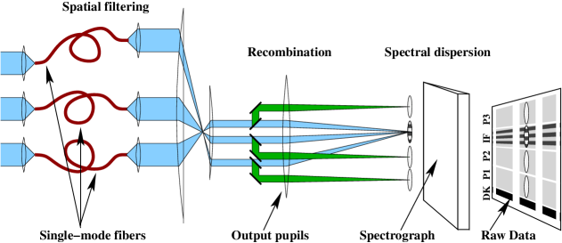
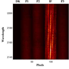
Figure 1: Left panel: Sketch of the AMBER instrument. The light enters the instrument from the left and is propagating from left to right, until the raw data are recorded on the detector. Further details are given in the text. Right panel: AMBER reconstituted image from the raw data recorded during the 3-telescope observation of the calibrator HD135382 in February 2005, in the medium spectral resolution mode. DK corresponds to a dark region, Pk are the vertically dispersed spectra obtained from each telescope and IF is the spectrally dispersed interferogram.

2 Presentation of the instrument

2.1 Image formation

The process of image formation of AMBER is sketched on Fig. 1 (left) from a signal processing point of view. It consists in three major steps. First, the beams from the three telescopes are filtered by single mode fibers to convert phase fluctuations of the corrugated wavefronts into intensity fluctuations that are monitored. The fraction of light entering the fiber is called the coupling coefficient (Shaklan & Roddier 1988) and depends on the Strehl ratio (Coudé du Foresto et al. 2000). At this point, a pair of conjugated cylindrical mirrors compresses by a factor of about 12 the individual beams exiting from fibers into one dimensional elongated beams to be injected in the entrance slit of the spectrograph. For each of the three beams, beam-splitters placed inside the spectrograph select part of the light and induce three different tilt angles so that each beam is imaged at different locations of the detector. These are called photometric channels and are each one relative to a corresponding incoming beam. The remaining parts of the light of the three beams are overlapped on the detector image plane to form fringes. The spatial coding frequencies of the fringes $f$ are fixed by the separation of the individual output pupils. They are respectively $f=[1,2,3]d/\lambda$, where $d$ is the output pupil diameter. Since the beams hit a spectral dispersing element (a prism glued on a mirror or one of the two gratings) in the pupil plane, the interferogram and the photometries are spectrally dispersed perpendicularly to the spatial coding. The dispersed interferogram arising from the beam combination, as well as the photometric outputs are recorded on the infrared detector, which characteristics are given in Table 1.

Table 1: Detector properties.

Detector specifications
Society/Name	Rockwell/HAWAII
Composition	HgCdTe
Number of pixels	$512\times 512$
Pixel size	$18.5\mu\mathrm{m}\times 18.5\mu\mathrm{m}$
Spectral width	$0.8\mu\mathrm{m}-2.5\mu\mathrm{m}$
Readout noise	$9\mathrm{e}^{-}$
$e^{-}/ADU$	4.18
Cooling	Liquid nitrogen
Temperature	$78\mathrm{K}$
Autonomy of cryostat	$24\mathrm{h}$

The detector consists in a 512 x 512 pixel array with the vertical dimension aligned with the wavelength direction. The first 20 pixels of each scanline of the detector are masked and never receive any light, allowing to estimate the readout noise and bias during an exposure. The light from the two (resp. 3) telescopes comes in three (resp. 4) beams, one ”interferometric” beam where the interference fringes are located, and two (resp. three) ”photometric” beams. These 3 (resp. 4) beams are dispersed and spread over three (resp. 4) vertical areas on the detector. The detector is read in subwindows. Horizontally, these subwindows are centered on the regions where the beams are dispersed, with a typical width of 32 to 40 pixels. Vertically, the detector can be set up to read up to three subwindows (covering up to three different wavelength ranges). The Raw Data format used by AMBER records individually these subframes. However, as sketched in the right panel of Fig. 1, the AMBER Raw Data can be conceived as the grouping together of these subwindows:

• the left column (noted “DK” ) , contains the masked pixels.

• the two following columns (noted “P1” and “P2”), and the right one in the three telescope mode (noted “P3”), of usually $32$ pixels wide, are the photometric outputs. They record the photometric signal coming from the three telescopes. When dealing with 2-telescope observations, only channels P1 and P2 are enlighted.

• the fourth column is the interferometric output (noted “IF”). it exhibits the interference fringes arising from the recombination of the beams (that is two or three beams, according to the number of telescopes used). We call $N_{pix}$ the number of pixels in this column, which is usually $N_{pix}=32$.

The individual image which is recorded during the detector integration time (DIT) is called a frame. A cube of frames obtained during the exposure time is called an exposure.

2.2 AMBER interferometric equation

The following demonstration is given considering a generic $N_{tel}\geq 2$ telescope interferometer. In the specific case of AMBER however, $N_{tel}=2$ or $N_{tel}=3$ only. Each line of the detector being independent with respect to each other, we can focus our attention on one single spectral channel, which is assumed here to be monochromatic. The effect of a spectral bandwidth on the interferometric equation is treated in Section 3.6.1.

Interferometric output: when only the $i^{th}$ beam is illuminated, the signal recorded in the interferometric channel is the photometric flux $F^{i}$ spread on the Airy pattern $a^{i}_{k}$, that is the diffraction pattern of the $i^{th}$ output pupil weighted by the single mode of the fiber. $k$ is the pixel number on the detector, $\alpha$ being the associated angular variable. $F^{i}$ results in the total source photon flux $N$ attenuated by the total transmission of the $i^{th}$ optical train $t^{i}$, i.e. the product of the optical throughput (including atmosphere and optical train of the VLTI and the instrument) and the coupling coefficient of the single mode fiber:

$$F^{i}=Nt^{i}$$ (1)

When beams $i$ and $j$ are illuminated simultaneously, the coherent addition of both beams results in an interferometric component superimposed to the photometric continuum. The interferometric part, that is the fringes, arises from the amplitude modulation of the coherent flux $F_{c}^{ij}$ at the coding frequency $f^{ij}$. The coherent flux is the geometrical product of the photometric fluxes, weighted by the visibility:

$$F_{c}^{ij}=2N\sqrt{t^{i}t^{j}}V^{ij}\mathrm{e}^{i(\Phi^{ij}+\phi_{p}^{ij})}$$ (2)

where $V^{ij}\mathrm{e}^{i\Phi^{ij}}$ is the complex modal visibility (Mège et al. 2003) and $\phi_{p}^{ij}$ takes into account a potential differential atmospheric piston. Note that strictly speaking the modal visibility is not the source visibility. However the study of the relation between the modal visibility and the source visibility is beyond the scope of this paper, and further informations can be found in Mège et al. (2003) and Tatulli et al. (2004). Here we consider our observable to be the complex modal visibility.

Such an analysis can be done for each pair of beams arising from the interferometer. As a result, the interferogram recorded on the detector can be written in the general form:

$$i_{k}=\sum_{i}^{N_{tel}}a^{i}_{k}F^{i}+\sum_{i<j}^{N_{tel}}\sqrt{a^{i}_{k}a^{j}_{k}}C^{ij}_{B}\mathrm{Re}\left[F_{c}^{ij}\mathrm{e}^{i(2\pi\alpha_{k}{f^{ij}}+\phi^{ij}_{s}+\Phi^{ij}_{B})}\right]$$ (3)

$\phi^{ij}_{s}$ is the instrumental phase taking into account possible misalignment and/or differential phase between the beams $a^{i}_{k}$ and $a^{j}_{k}$. $C^{ij}_{B}$ and $\Phi^{ij}_{B}$ are respectively the loss of contrast and the phase shift due to polarization mismatch between the two beams (after the polarizers), as rotation of the single mode fibers might induce. This equation is governing the AMBER fringe pattern, that is the interferometric channel of the fourth column. The first sum in Eq. (3), which represents the continuum part of the interference pattern, is called from now on the DC component, and the second sum, which describes the high frequency part (that is the coded fringes), is called the AC component of the interferometric output.

Photometric outputs: thanks to the photometric channels, the number of photoevents $p^{i}(\alpha)$ coming from each telescope can be estimated independently:

$$p^{i}_{k}=F^{i}b^{i}_{k}$$ (4)

where $b^{i}_{k}$ is the beam profile in the $i^{th}$ photometric channel. The previous equation rules the photometric channels.

3 Data reduction algorithm

The AMBER data reduction algorithm is based on the modelling of the interferogram in the detector plane. Such a method requires an accurate calibration of the instrument.

3.1 Modelling the interferogram

In order to model the interferogram, we discriminate between the astrophysical and instrumental parts in the interferometric equation. It comes

$$i_{k}=\sum_{i}^{N_{tel}}a^{i}_{k}F^{i}+\sum_{i<j}^{N_{tel}}\left[c_{k}^{ij}{R^{ij}}+d_{k}^{ij}{I^{ij}}\right]$$ (5)

with

$$c_{k}^{ij}=C^{ij}_{B}\frac{\sqrt{a^{i}_{k}a^{j}_{k}}}{\sqrt{\sum_{k}a_{k}^{i}a_{k}^{j}}}\cos(2\pi\alpha_{k}{f^{ij}}+\phi^{ij}_{s}+\Phi^{ij}_{B})$$ (6)

$$d_{k}^{ij}=C^{ij}_{B}\frac{\sqrt{a^{i}_{k}a^{j}_{k}}}{\sqrt{\sum_{k}a_{k}^{i}a_{k}^{j}}}\sin(2\pi\alpha_{k}{f^{ij}}+\phi^{ij}_{s}+\Phi^{ij}_{B})$$ (7)

and

$${R^{ij}}=\sqrt{\sum_{k}a_{k}^{i}a_{k}^{j}}\mathrm{Re}\left[F_{c}^{ij}\right],\leavevmode\nobreak\ \leavevmode\nobreak\ {I^{ij}}=\sqrt{\sum_{k}a_{k}^{i}a_{k}^{j}}\mathrm{Im}\left[F_{c}^{ij}\right]$$ (8)

As an analogy with telecom data processing, $c_{k}^{ij}$ and $d_{k}^{ij}$ are called the carrying waves of the signal at the coding frequency $f^{ij}$, since they carry (in terms of amplitude modulation) $R^{ij}$ and $I^{ij}$, which are directly linked to the complex coherent flux (as shown by Eq. (8)).

The estimated photometric fluxes $P^{i}$ are computed from the photometric channels (see Eq. (4)):

$$P^{i}=F^{i}\sum_{k}b_{k}^{i}$$ (9)

If we know the ratio $v_{k}^{i}$ –which depends only of the instrumental configuration – between the measured photometric fluxes $P^{i}$ and the corresponding DC components of the interferogram, we can have an estimation of the latter thanks to the following formula:

$$a^{i}_{k}F^{i}=P^{i}v_{k}^{i}$$ (10)

We then can compute the DC continuum corrected interferogram $m_{k}$:

$$m_{k}=i_{k}-\sum_{i=1}^{N_{tel}}P^{i}v_{k}^{i}$$ (11)

which can be rewritten:

$$m_{k}=c_{k}^{ij}R^{ij}-d_{k}^{ij}I^{ij}$$ (12)

This equation defines a system of $N_{pix}$ linear equations with $2N_{b}=N_{tel}(N_{tel}-1)$ unknowns (i.e. twice the number of baselines). It characterizes the linear link between the pixels on the detector and the complex visibility:

$$\left(\begin{array}[]{c}m_{1}\\ |\\ m_{N_{pix}}\end{array}\right)=\overbrace{\left(\begin{array}[]{ccc}..&c_{1}^{ij}&..\\ |&:&|\\ ..&c_{N_{pix}}^{ij}&..\end{array}\right.}^{N_{b}}\overbrace{\left.\begin{array}[]{ccc}..&d_{1}^{ij}&..\\ |&:&|\\ ..&d_{N_{pix}}^{ij}&..\end{array}\right)}^{N_{b}}\left(\begin{array}[]{c}:\\ R^{ij}\\ :\\ I^{ij}\\ :\end{array}\right)=\mathrm{V2PM}\left(\begin{array}[]{c}:\\ R^{ij}\\ :\\ I^{ij}\\ :\end{array}\right)$$ (13)

The $\mathrm{V2PM}$ matrix (namely Visibility To Pixel Matrix), which contains the carrying waves, holds the information about the interferometric beams $\sqrt{a^{i}_{k}a^{j}_{k}}$, the coding frequencies $f^{ij}$ and the instrumental differential phases $\phi^{ij}_{s}$. Together with the $v_{k}^{i}$, they entirely describe the instrument from a signal processing point of view. These quantities, namely $c_{k}^{ij}$, $d_{k}^{ij}$ and $v_{k}^{i}$ have however to be calibrated.

3.2 Calibration procedure

Table 2: Acquisition sequence of calibration files

Step	Sh $1$	Sh $2$	Sh $3$	Phase $\gamma_{0}$	DPR key
1	O	X	X	NO	2P2V, 3P2V
2	X	O	X	NO	2P2V, 3P2V
3	O	O	X	NO	2P2V, 3P2V
4	O	O	X	YES	2P2V, 3P2V
5	X	X	O	NO	3P2V
6	O	X	O	NO	3P2V
7	O	X	O	YES	3P2V
8	X	O	O	NO	3P2V
9	X	O	O	YES	3P2V

Sh = Shutter; O = Open; X = Closed

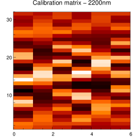
Figure 2: Outputs of the calibration procedures. Examples have been chosen for one given wavelength: $\lambda=2.2\mu\mathrm{m}$. Left: the $v_{k}^{i}$ functions. Middle: the matrix containing the carrying waves, the first three columns are the $c_{k}^{ij}$ functions for each baseline, and the three last columns are the respective $d_{k}^{ij}$ functions. One can see that for each baseline $c_{k}^{ij}$ and $d_{k}^{ij}$ are in quadrature. Right: another representation of the carrying waves. From top to bottom, both sinusoidal functions correspond respectively to columns $1-4$, $2-5$ and $3-6$ of the calibration matrix.

The calibration procedure is performed thanks to an internal source located in the Calibration and Alignment Unit (CAU) of AMBER (Petrov et al. 2006). It consists in acquiring a sequence of high signal-to-noise ratio calibration files, which successive configurations are summarized in Table 2 and detailed below. Since the calibration is done in laboratory, the desired level of accuracy of the measurements is insured by choosing the appropriate integration time. As an example, typical integrations time in “average accuracy” mode are (for the full calibration process) $\tau=17\mathrm{s},\leavevmode\nobreak\ 30\mathrm{s},\leavevmode\nobreak\ 800\mathrm{s}$ for respectively low, medium and high spectral resolution modes in the K band, and $100$ times higher for the “high accuracy” calibration mode.

The sequence of calibration files has been chosen to accommodate both two and three-telescope operations. For a two-telescope operation, only the 4 first steps are needed. Raw data FITS files produced by the ESO instruments bear no identifiable name and can only be identified as, e.g., files relevant to the calibration of the V2PM matrix, only by the presence of dedicated FITS keywords (ESO’s pipeline Data PRoduct keys or “DPR keys”) in their header. The DPR keys used are listed in Table 2.

First (steps $1$ and $2$—and $5$ when in 3-telescope mode), for each telescope beam, an image is recorded with only this shutter opened. The fraction of flux measured between the interferometric channel and the illuminated photometric channel leads to an accurate estimation of the $v_{k}^{i}$ functions. Then, in order to compute the carrying waves $c_{k}^{ij}$ and $d_{k}^{ij}$, one needs to have two independent (in terms of algebra) measurements of the interferogram since there are two unknowns (per baseline) to compute. The principle is the following: two shutters are opened simultaneously (respectively steps $3/4$, $6/7$, and $8/9$) and for each pair of beams, the interferogram is recorded on the detector. Such an interferogram corrected from its DC component and calibrated by the photometry yields the knowledge of the $c_{k}^{ij}$ carrying wave. To obtain its quadratic counterpart, the previous procedure is repeated by introducing a known phase shift close to $90$ degree $\gamma_{0}$ using piezoelectric mirrors at the entrance of beams 2 and 3. Computing the $d_{k}^{ij}$ function from the knowledge of $c_{k}^{ij}$ and $\gamma_{0}$ is straightforward. Note that by construction: (i) the carrying waves are computed with the unknown system phase $\Phi^{c}$ (possible phase of the internal source, differential optical path difference introduced at the CAU level, etc…), and that; (ii) since the internal source in the CAU is slightly resolved by the largest baseline (1–3) of the output pupils, the carrying waves for this specific baseline are weighted by the visibility $V_{c}$ of the internal source. Hence at this point, the carrying waves are following expressions slightly different from their original definition given by Eq.’s (6) and (7):

$$c_{k}^{ij}=\frac{\sqrt{a^{i}_{k}a^{j}_{k}}}{\sqrt{\sum_{k}a_{k}^{i}a_{k}^{j}}}C^{ij}_{B}V_{c}^{ij}\cos(2\pi\alpha_{k}{f^{ij}}+\phi^{ij}_{s}+\Phi^{ij}_{B}+\Phi^{ij}_{c})$$ (14)

$$d_{k}^{ij}=\frac{\sqrt{a^{i}_{k}a^{j}_{k}}}{\sqrt{\sum_{k}a_{k}^{i}a_{k}^{j}}}C^{ij}_{B}V_{c}^{ij}\sin(2\pi\alpha_{k}{f^{ij}}+\phi^{ij}_{s}+\Phi^{ij}_{B}+\Phi^{ij}_{c})$$ (15)

However, since $c_{k}^{ij}$ and $d_{k}^{ij}$ are shifted by $\pi/2$, they insure the following relation:

$$\sum_{k}^{N_{pix}}c_{k}^{2}+d_{k}^{2}=C_{B}^{2}V_{c}^{2}$$ (16)

Hence the conjugated loss of visibility due to the internal source and the polarization effects can be known and calibrated by computing previous formula. Unfortunately, since it is not possible to disentangle between both contrast losses, and since the $V_{c}$ factor only affects the interferograms arising from the calibration procedure, and not from the observation, the visibility estimated on a star will be affected from this factor as well, as shown in Section 3.5.1.

Figure 3 illustrates Eq. 16. For the baselines $(1,2)$ and $(2,3)$, the contrast loss arises from polarization effects since the internal source is unresolved. We find respectively $C_{B}^{12}\simeq 0.9$, and $C_{B}^{23}\simeq 0.8$. For the third baseline $(1,3)$, the internal source is partially resolved, which explain an higher contrast loss, $C_{B}^{13}V_{c}^{13}\simeq 0.7$.

3.3 Fringe fitting

To estimate the coherent fluxes $R^{ij}$ and $I^{ij}$ which are at the basis of the computation of the whole AMBER observables, one has to solve the inverse problem described by Eq. (13), that is one has to perform a $\chi^{2}$ linear fit of the fringes, with the coherent fluxes being the unknown parameters. The solution is given by the following equation:

$$[\widetilde{R}^{ij},\widetilde{I}^{ij}]=\mathrm{P2VM}[m_{k}]$$ (17)

where

$$\mathrm{P2VM}=[\mathrm{V2PM}^{T}\mathcal{C}_{M}^{-1}{\bf\mathrm{V2PM}}]^{-1}\mathrm{V2PM}^{T}\mathcal{C}_{M}^{-1}$$ (18)

is the generalized inverse of the $\mathrm{V2PM}$ matrix, $\mathcal{C}_{M}$ being the covariance matrix of the measurements $m_{k}$, and $X^{T}$ denoting the transpose of the $X$ matrix. P2VM means Pixel to Visibility Matrix since it allows to estimate the complex visibility from the interferogram recorded on the detector. Assuming that the pixels on the detector are uncorrelated, the $\mathcal{C}_{M}$ matrix is diagonal, with each term of the diagonal being defined by the variance of the DC corrected interferogram $\sigma^{2}(m_{k})$. The fundamental error on the DC corrected interferogram arises from the photon noise and detector noise (of variance $\sigma$) corrupting the measurements, that is each pixel of the interferogram $i_{k}$, and the estimated photometric fluxes $P^{i}$. It comes:

$$\sigma^{2}(m_{k})=\overline{i_{k}}+\sigma^{2}+\sum_{i=1}^{N_{tel}}\left[\overline{P_{i}}+N_{pix}\sigma^{2}\right](v^{i}_{k})^{2}$$ (19)

3.4 Fringe detection

Positive detection of fringes in the measurements requires at the same time enough flux entering the fibers and high enough fringe contrast, so that the fringes rise of the noise level. As a result, the computation of the signal to noise ratio of the coherent flux, which takes into account both of the parameters, appears naturally as the relevant criterion to use. It writes:

$$\mathrm{SNR}^{2}(t)=\frac{1}{N_{b}}\frac{1}{N_{l}}\sum_{b}^{N_{b}}\sum_{l}^{N_{l}}\left[\left(\frac{{R^{b}}^{2}(l,t)}{\sigma^{2}_{R^{b}}}-1\right)+\left(\frac{{I^{b}}^{2}(l,t)}{\sigma^{2}_{I^{b}}}-1\right)\right]$$ (20)

$b$ being for sake of simplicity the baseline number which describes each couple of telescopes $(i,j)$, $N_{b}$ being the number of baselines, and $N_{l}$ being the number of spectral channels. In absence of fringes, the quantities ${R^{b}}^{2}$ and ${I^{b}}^{2}$ are tending toward $\sigma^{2}_{R^{b}}$ and $\sigma^{2}_{I^{b}}$ respectively, thus driving the fringe criterion toward $0$. At the opposite, the presence of fringes above the noise level, that is when ${R^{b}}^{2}(l,t)>\sigma^{2}_{R^{b}}$ and/or ${I^{b}}^{2}(l,t)>\sigma^{2}_{I^{b}}$ imposes the fringe criterion to be strictly superior to $0$ and is directly linked to the quality of the frames. It thus allows to operate a fringe selection prior to the proper estimation of the observables, which step can be useful for sets of data recorded in bad observational conditions, as shown in Section 5.2.

$\sigma^{2}_{R^{b}}$ and $\sigma^{2}_{I^{b}}$, that is the bias part of respectively $R^{2}$ and $I^{2}$, can be easily computed from the definition of the real and imaginary part of the coherent fluxes, which are linear combinations of the DC continuum corrected interferograms $m_{k}$. If $\zeta^{b}_{k}$ and $\xi^{b}_{k}$ are the coefficient of the P2VM matrix, $R^{b}$ and $I^{b}$ verify the respective following equations:

$$R^{b}=\sum_{k=1}^{N_{pix}}\zeta^{b}_{k}m_{k},\leavevmode\nobreak\ \leavevmode\nobreak\ I^{b}=\sum_{k=1}^{N_{pix}}\xi^{b}_{k}m_{k}$$ (21)

It comes straightforward that:

$$\sigma^{2}_{R^{b}}=\sum_{k}(\zeta^{b}_{k})^{2}\sigma^{2}(m_{k});\leavevmode\nobreak\ \sigma^{2}_{I^{b}}=\sum_{k}(\xi^{b}_{k})^{2}\sigma^{2}(m_{k})$$ (22)

Figure 3: Contrast loss due to polarization effects and partial resolution of the internal source, as a function of the wavelength. The 3-telescope P2VM used is the same than the one presented in Fig. 2. The errors bars are roughly at the level of the contrast loss rms along the wavelength. In other words, the contrast loss is constant over the wavelength range.

3.5 Estimation of the observables

For each spectral channel, squared visibility and closure phase (in the three telescope case) can be estimated from the interferogram. Taking advantage of the spectral dispersion, differential phase can be computed as well. In the following paragraphs, we denote with $\left<...\right>$ the ensemble average of the different quantities. This average can be performed either on the frames within an exposure and/or on the wavelengths.

3.5.1 The squared visibility

Theoretically speaking, the squared visibility is given by computing the ratio between the squared coherent flux and the photometric fluxes. Following Eq.’s (1), (2), (8) and (9) it comes:

$$\frac{|F_{c}^{ij}|^{2}}{4F^{i}F^{j}}=\frac{{R^{ij}}^{2}+{I^{ij}}^{2}}{4P^{i}P^{j}\sum_{k}v_{k}^{i}v_{k}^{j}}=\frac{|V^{ij}|^{2}}{{V_{c}^{ij}}^{2}}$$ (23)

Note that, thanks to the calibration process, the computed visibility is free from the instrumental contrast, that is the loss of contrast due to the instrument, but as mentioned in Section 3.2, the object visibility is weighted by the visibility of the internal source. However this factor (${V_{c}^{ij}}^{2}$) automatically disappears when doing the necessary atmospheric calibration (see Section 3.6.2).

As a result the visibility – atmospheric issues apart – has still to be calibrated by observing a reference source.

In practice, because data are noisy, we perform an ensemble average on the frames that compose the data cube (see Section 2.1) to estimate the expected values of the square coherent flux and the photometric fluxes, respectively. Taking the average of the squared modulus of the coherent flux, that is doing a quadratic estimation, allows to handle the problem of the random differential piston $\phi_{p}^{ij}$, but introduces a quadratic bias due to the zero-mean photon and detector noises (Perrin 2003). The expression of the squared visibility estimator, unbiased by fundamental noises is therefore:

$$\frac{\widetilde{|V^{ij}|^{2}}}{{V_{c}^{ij}}^{2}}=\frac{\left<{R^{ij}}^{2}+{I^{ij}}^{2}\right>-\leavevmode\nobreak\ \mathrm{Bias}\{{R^{ij}}^{2}+{I^{ij}}^{2}\}}{4\left<P^{i}P^{j}\right>\sum_{k}v_{k}^{i}v_{k}^{j}}$$ (24)

The quadratic bias of the squared amplitude of the coherent flux writes as the quadratic sum of the biases of $R^{2}$ and $I^{2}$. From Eq. 22, it comes:

$$\mathrm{Bias}\{{R^{ij}}^{2}+{I^{ij}}^{2}\}=\sum_{k}\left[(\zeta^{ij}_{k})^{2}+(\xi^{ij}_{k})^{2}\right]\sigma^{2}(m_{k})$$ (25)

Previous equation is nothing but the mathematical expression that describes the bias as the quadratic sum of the errors of the measurements $\sigma^{2}(m_{k})$ (as defined by Eq. (19)), projected on the real and imaginary axis of the coherent flux.

Using the squared visibility estimator of Eq. (24), the theoretical error bars on the squared visibility can be computed from its second order Taylor expansion (Papoulis 1984; Kervella et al. 2004):

$$\sigma^{2}(|V^{ij}|^{2})=\frac{1}{M}\left[\frac{\sigma^{2}(|C^{ij}|^{2})}{\overline{|C_{ij}|^{2}}^{2}}+\frac{\sigma^{2}(P^{i}P^{j})}{\overline{P^{i}P^{j}}^{2}}\right]\overline{|V^{ij}|^{2}}^{2}$$ (26)

where $|C^{ij}|^{2}={R^{ij}}^{2}+{I^{ij}}^{2}-\leavevmode\nobreak\ \mathrm{Bias}\{{R^{ij}}^{2}+{I^{ij}}^{2}\}$ is the unbiased squared coherent flux. In practice, the expected value and the variance of the squared coherent flux and the photometric fluxes are computed empirically from the $M$ available measurements. It comes the following semi-empirical formula:

$$\sigma_{stat}^{2}(\widetilde{|V^{ij}|^{2}}) = \frac{1}{M}\left[\frac{\left<|C^{ij}|^{4}\right>_{M}-\left<|C^{ij}|^{2}\right>^{2}_{M}}{\left<|C^{ij}|^{2}\right>^{2}_{M}}\right.$$ (27)

$$+ \left.\frac{\left<{P^{i}}^{2}{P^{j}}^{2}\right>_{M}-\left<P^{i}P^{j}\right>^{2}_{M}}{\left<P^{i}P^{j}\right>^{2}_{M}}\right]\widetilde{|V^{ij}|^{2}}^{2}$$

Note finally that, although quadratic estimation of the visibility has been computed, the squared visibility will be systematically decreased by the atmosphere jitter during the frame integration time. We focus on this effect in Sect. 3.6.

3.5.2 The closure phase

By definition, the closure phase is the phase of the so-called bispectrum ${B}^{123}$. The latter results on the ensemble average of the coherent flux triple product and then estimated as follows:

$$\widetilde{B}^{123}=\left<C^{12}C^{23}{C^{13}}^{\ast}\right>$$ (28)

where $C^{ij}=R^{ij}+iI^{ij}$. The closure phase then comes straightforward:

$$\widetilde{\phi_{B}}^{123}=\mathrm{atan}\left[\frac{\mathrm{Im}(\widetilde{B}^{123})}{\mathrm{Re}(\widetilde{B}^{123})}\right]$$ (29)

The closure phase presents the advantage to be independent of the atmosphere (e.g. Roddier (1986)). However in the case of AMBER, the closure phase of the image might not coincide with the one of the object and might be biased because of the calibration process. If the so-called system phase presents an non zero closure phase $\Phi_{c}^{12}+\Phi_{c}^{23}-\Phi_{c}^{13}$, this bias must be calibrated by observing a point source or at least a centro-symmetrical object. So far, no theoretical computation of the error of the closure phase has been provided for the AMBER data reduction algorithm. Thus, closure phases internal error bars (i.e. that does not include systematics errors) are computed statistically, that is by taking the root mean square of all the individual frames, then divided by the square root of the number of frames, as it is illustrated in Section 5.5.

3.5.3 The differential phase

The differential phase is the phase of the so-called cross spectrum ${W}_{12}$. For each baseline, the latter is estimated from the complex coherent flux taken at two different wavelengths $\lambda_{1}$ and $\lambda_{2}$:

$$\widetilde{W_{12}^{ij}}=\left<C^{ij}_{\lambda_{1}}{C^{ij}_{\lambda_{2}}}^{\ast}\right>\\$$ (30)

And the differential phase is:

$$\widetilde{\Delta\phi_{12}^{ij}}=\mathrm{atan}\left[\frac{\mathrm{Im}\left(\widetilde{W_{12}^{ij}}\right)}{\mathrm{Re}\left(\widetilde{W_{12}^{ij}}\right)}\right]$$ (31)

3.5.4 The piston

The interferometric phase induced by the achromatic piston term takes the form:

$$\phi^{ij}_{\lambda}=\frac{2\pi\delta^{ij}}{\lambda}={2\pi\delta^{ij}\sigma}$$ (32)

where $\delta^{ij}$ is the achromatic differential piston between telescope i and j, $\lambda$ is the wavelength and $\sigma$ is the wavenumber (i.e. $\sigma=1/\lambda$).
First order Taylor expansion: At first order, the estimated differential phase of Eq. (31) is a linear function which takes the generic form $\Delta\phi_{12}=\phi_{1}+2\pi\left(\sigma_{2}-\sigma_{1}\right)\delta$. Its slope $\delta$ depends of the sum of atmospheric piston $\delta_{p}$ which varies frame by frame, and of the linear component of the object differential phase $\delta_{o}$. A good estimate of this slope in presence of noise is the argument of the average cross spectrum along the wavelengths:

$$\widetilde{\delta^{ij}_{p}}+\widetilde{\delta^{ij}_{o}}=\frac{{\rm arg}\left<W_{\lambda_{2l},\lambda_{2l+1}}^{ij}\right>_{l}}{2\pi\left<\sigma_{\lambda_{2l+1}}-\sigma_{\lambda_{2l}}\right>_{l}}$$ (33)

The estimation of the piston is unbiased when the wave number varies linearly with the spectral pixel index (linear grating dispersion law). This can be true with an excellent approximation at Medium Spectral Resolution and High Spectral Resolution in the AMBER case. However, for the Low Spectral Resolution, biases as high as 5% in the estimation of piston can occur.
Fitting the complex phasor: The achromatic piston can also be estimated from a least square fit of the complex coherent flux. If we define the complex phasor as:

$$\Psi_{\lambda}=C_{\lambda}^{ij}\times e^{\frac{2i\pi\delta^{ij}}{\lambda}}$$ (34)

$\delta^{ij}$ can be retrieved by minimizing the phase of such complex phasor, or equivalently by minimizing the tangent of the phase. The $\chi^{2}$ is then defined as:

$$\chi^{2}=\frac{\displaystyle\sum_{\lambda}\frac{\left(\frac{\mathrm{Im}\left(\Psi_{\lambda}\right)}{\mathrm{Re}\left(\Psi_{\lambda}\right)}\right)^{2}}{\sigma^{2}_{R_{\lambda}}+\sigma^{2}_{I_{\lambda}}}}{\displaystyle\sum_{\lambda}\frac{1}{\sigma^{2}_{R_{\lambda}}+\sigma^{2}_{I_{\lambda}}}}$$ (35)

This $\chi^{2}$ is highly non-linear and simple techniques as gradient fitting cannot be used here. On the contrary, non-linear fitting techniques such as genetic or simulated annealing algorithms (Kirkpatrick et al. 1983) must be used instead.

Note that, in order to disentangle between the atmospheric piston $\delta_{p}$ and the linear component of the differential phase $\delta_{o}$, the fitting techniques described above can be performed only using spectral channels corresponding to the continuum of the source (i.e. outside spectral features), that is where its differential phase of the object is assumed to be zero.

3.6 Biases of the visibility

3.6.1 Loss of spectral coherence

The above derivation of the interferometric equation assumes a monochromatic spectral channel. In practice the spectral width of one spectral channel is non zero and depends on the resolution $\mathcal{R}$ of the spectrograph. As a consequence the coherence length $\mathcal{L}_{c}$ of the interferogram is finite and equals $\mathcal{L}_{c}=\lambda_{0}\mathcal{R}$ where $\lambda_{0}$ is the reference wavelength in the spectral channel. Assuming a linear decomposition of the phase of the interferogram and neglecting higher orders, the interferogram is attenuated by a factor $\rho_{k}$, which can be written:

$$\rho_{k}=\left|\widehat{\mathcal{F}}\left(\pi\frac{\delta_{k}+\delta_{p}+\delta_{o}}{\mathcal{L}_{c}}\right)\right|$$ (36)

where $\widehat{\mathcal{F}}$ is the Fourier transform of the spectral filter function. $\delta_{k}$ is the spatial sampling of the interferogram, that is the pixel coordinates expressed in optical path difference (OPD) units, $\delta_{p}$ and $\delta_{o}$ being respectively the atmospheric piston and the slope of the object spectral differential phase, as defined in Sect. 3.5.4. Note that for a square filter, the attenuation coefficient takes the well known form of the sinc function:

$$\rho_{k}=\left|\mathrm{sinc}\left(\pi\frac{\delta_{k}+\delta_{p}+\delta_{o}}{\mathcal{L}_{c}}\right)\right|$$ (37)

In the low resolution mode where $\mathcal{R}=35$, the attenuation coefficient severely depends on the pixel position $\delta_{k}$ which is calibratable quantity. Nonetheless, the compensation of this effect requires an iterative process in two steps where (i) the estimation of $\delta_{p}+\delta_{o}$ is performed as described in Section 3.5.4, and (ii) the $\rho_{k}$ attenuation correction is applied directly to the DC corrected interferograms $m_{k}$. The loop is then repeated until convergence. This algorithm, which not yet implemented in the software, will be described in greater details in a further paper.

In the medium and high resolution (where respectively $\mathcal{R}=1500$ and $\mathcal{R}=10000$) however, the OPD $\delta_{k}$ due the spatial sampling of AMBER can be neglected. Indeed this approximation drives to a relative error of the coefficient below $10^{-3}$ and $10^{-5}$ respectively, that is within the specified error bars of the visibility. In such a case, the loss of spectral coherence simply results in biasing frame to frame the visibility by a factor $\rho(\delta_{p}+\delta_{o})$. This bias can be corrected by knowing the shape of the spectral filter and by estimating the piston $\delta_{p}+\delta_{o}$ thanks to Eq. (33).

3.6.2 Atmospheric jitter

Although a quadratic estimation of the visibility has been performed to avoid the differential piston to completely cancel out the fringes, the high frequency variations of the latter during the integration time – so called high-pass jitter – nevertheless blur the fringes. As a result, the coherent flux, hence the visibility, is attenuated. In average, the attenuation coefficient $\Gamma$ of the squared visibility is given by Colavita (1999b):

$$\Gamma=\exp(-\sigma^{2}_{\phi^{p}_{hf}})$$ (38)

where $\sigma^{2}_{\phi^{p}_{hf}}$ is the variance of the high-pass jitter $\phi^{p}_{hf}$.

For the time being, this atmospheric effect is compensated by calibrating the source visibility with a reference source observed shortly before and after the scientific target to insure similar atmospheric conditions. We have also planned to provide in the near future a more accurate calibration of this effect, based on the computation of the variance of the so-called “first difference phase jitter”, that is the difference of the average piston taken between two successive exposures, as proposed by Colavita (1999b) for the PTI interferometer and successfully applied by Malbet et al. (1998). However, jitter analysis (as it is illustrated in Section 5.2) cannot be tested and validated as long as the extra-sources of vibrations due to VLTI instabilities (delay lines, adaptive optics…), hardly calibratable, are clearly identified and suppressed. Note as well that the use of the accurate fringe tracker FINITO (Gai et al. 2002), soon expected to operate on the VLTI, should drastically reduce the jitter attenuation, hence allowing to integrate on times much longer than the coherence time of the atmosphere in order to reach fainter stars.

4 The amdlib data reduction software

A dedicated software to reduce AMBER observations has been developed by the AMBER consortium. This consists in a library of C functions, called amdlib, plus high-level interface programs. The amdlib functions are used at all stages of AMBER data acquisition and reduction: in the Observation Software (OS) for wavelength calibration and fringe acquisition, in the (quasi) Real Time Display program used during the observations, in the online Data Reduction Pipeline customary for ESO instruments, and in various offline front end applications, noticeably a Yorick implementation (AmmYorick). The amdlib library is meant to incorporate all the expertise on AMBER data reduction and calibration acquired throughout the life of the instrument, bound to evolve with time.

The data obtained with AMBER (“raw data”) consist in an exposure, i.e., a time series of frames read on the infrared camera, plus all relevant information from AMBER sensors, observed object, VLTI setup, etc…, stored in FITS TABLE format, according to ESO interface document VLT-ICD-ESO-15000-1826. Saving the raw, uncalibrated data, although more space consuming, permits to benefit afterward, by replaying the calibration sequences and the data reduction anew, of all the improvements that could have been deposited in amdlib in the meantime.

The library contains a set of “software filters” that refine the raw data sets to obtain calibrated “science data frames”. This treatment is performed on every raw data frames, irrespective of their future use (calibration or observation). A second set of functions perform high level data extraction on these calibrated frames, either to compute the V2PM (see Sect. 4.3) from a set of calibration data, or to extract the visibilities from a set of science target observations, the end product in this case being a reduced set of visibilities per object, stored in the optical interferometry standard $\mathrm{OI\_FITS}$ format (Pauls et al. 2005).

4.1 Detector calibration

First, all frames pixels are tagged valid if not present in the currently available bad pixel list of the AMBER detector. Then they are converted to photoevent counts. This step necessitates, for each frame, to model precisely the spatially and temporarily variable bias added by the electronics. The detector exhibits a pixel-to-pixel (high frequency) bias whose pattern is constant in time but depends on the detector integration time (DIT) and the size and location of the subwindows read on the detector. Thus, after each change in the detector setup, a new pixel bias map (PBM) is measured prior to the observations by averaging a large number of frames acquired with the detector facing a cold shutter. This PBM is then simply removed from all frames prior to any other treatment.

Once this fixed pattern has been removed, the detector may still be affected by a time-variable “line” bias, i.e., a variable offset for each detector line. This bias is estimated for each scan line and each frame as the mean value of the corresponding line of masked pixels (“DK” column in Fig. 1), and substracted from the rest of the line of pixels. The detector has an image persistence of $\sim 10\%$, consequently all frames are corrected from this effect before calibration. Pixels are then converted to photoevent counts by multiplying by the pixel’s gain. Currently the map of the pixels gains used is simply a constant $e^{-}/ADU$ value (see Table 1) multiplied by a “flat field” map acquired during laboratory tests.

Finally, the rms of the values in the masked pixel set, that were calibrated as the rest of the detector, gives the frame’s detector noise.

4.2 Image alignment and science data production

Once the cosmetics on the pixels is done, amdlib corrects the data from the spatial distortions present in the image. Presently, the only effect corrected is a displacement of the spectra acquired in the “photometric channels” (labeled P1, P2, P3 in Fig. 1) with regards to the fringed spectrum in the interferometric channel. This displacement, of a few pixels in the spectral dispersion direction, is due to a slight misalignment of the beam-splitters described in Sect. 2.1, and correcting from this effect is mandatory to compute the DC continuum interferogram (Eq. (11)). The calibration of this displacement is performed by amdlib during the spectral calibration procedure, one of the first calibration sequences to be performed prior to observations.

Finally, each frame is converted to the more handy “science data” structure, that contains only the calibrated image of the “interferometric channel” and (up to) three 1D vectors, the corresponding instantaneous photometry of each beam, corrected from the above mentioned spectral displacement.

4.3 Calibration matrix computation

The computation of the V2PM matrix is performed by the function amdlibComputeP2vm(). This function processes the 4 or 9 files described in Sect. 3.2, applying on each of them the detector calibration, image alignment and conversion to “science data” described above, then computing the $v_{k}^{i}$ (Eq. (10)) and the carrying waves $c_{k}^{ij}$ and $d_{k}^{ij}$ of the V2PM matrix (Eq. (13)). The result is stored in a FITS file, improperly called, for historical reasons, “the P2VM”.

The P2VM matrix is the most important set of calibration values needed to retrieve visibilities. The shape of the carrying waves (the $c_{k}$s and $d_{k}$s ) and in a lesser measure the associated $v_{k}$s, are the imprints of all the changes in intensity and phase that the beams suffer between the output of each fiber and the detection on the infrared camera. Any change in the AMBER optics situated in this zone, either by moving, e.g., a grating, or just thermal long-term effects, render the P2VM unusable. Thus, the P2VM matrix must be recalibrated each time a new spectral setup is called that involves changing the optical path behind the fibers.

All the instrument observing strategies and operation are governed by the need to avoid unnecessary optical changes, and care is taken at the operating system level to insure a recalibration of the P2VM whenever a “critical” motor affecting the optical path is set in action. To satisfy these needs, the P2VM computation has been made mandatory prior to science observations, and is given an unique ID number. All the science data files produced after the P2VM file inherit of this ID, that associates them with their “governing” calibration matrix. The amdlib library takes the opportunity that the P2VM file is pivotal to the data reduction, and unique, to make it a placeholder of all the other calibration tables needed to reduce the science data, namely the spectral calibration, bad pixels and flat field tables.

4.4 From science data to visibilities

The computation of visibilities is performed by the amdlibExtractVisibilities() function, using a valid P2VM file. amdlibExtractVisibilities() is able to perform visibility estimates on a frame-by-frame basis, or over a group of frames, called bin.

The amdlibExtractVisibilities() function, in sequence:

1. invert the V2PM calibration matrix;

2. extract Raw Visibilities;

3. correct from Biases, compute debiased $V^{2}$ visibilities,

4. compute Phase Closures,

5. compute Cross Spectra

6. fit Piston values from cross spectra

7. write the OI-FITS output file.

A typical data reduction process will first process all raw data files related to the calibration procedures performed before acquiring the science data, thus performing spectral calibration (e.g., using the command line program amdlibComputeSpectralCalibration), then P2VM file computation (e.g., using the command line program amdlibComputeP2vm). Once the P2VM file is computed, it contains all the calibration quantities necessary to process science object observations. One then uses the amdlibExtractVis program on a science data set to get the final OI-FITS file containing the measured science object visibilities.

5 Illustrations and discussions

This section aims to present step by step the data reduction procedures performed on real interferometric measurements arising from VLTI observations. Results are discussed, focusing on key points of the process.

5.1 Fringe fitting

Figure 4: Example of fringe-fitting by the carrying waves, in the $3$ telescope case. The DC corrected interferogram is plotted (dashdot line) with the error bars. The result of the fit is overplotted (solid line).

Assuming the calibration process has been properly performed following Section 3.2, the first step in the derivation of the observables is to estimate the real and imaginary part of the coherent flux. This is done by inverting the calibration matrix and obtaining the P2VM matrix, shown by Eq.’s (17) and (18). Figure 4 gives an example of the fringe fitting process, for an observation of the calibrator star HD135382 with three telescopes.

However, before going further in the data reduction process, it might be worthwhile for the users to check the validity of the fit and then to detect any potential problems in the data. Such step can be easily done by computing the residual $\chi^{2}_{res}$ between the measurements $m_{k}$ and the model $\widetilde{m}_{k}$:

$$[\widetilde{m}_{k}]=\mathrm{V2PM}[\widetilde{R}^{ij},\widetilde{I}^{ij}]$$ (39)

and

$$\chi^{2}_{res}=[\widetilde{m}_{k}-m_{k}]^{T}\mathcal{C}_{M}^{-1}[\widetilde{m}_{k}-m_{k}]$$ (40)

Using this checking procedure, the user can verify two critical points of the data processing:

• the correct subtraction of the DC component (see Eq. (11)): if such a condition is not fulfilled, the computed visibility will inevitably be biased since the fringe fitting by the carrying waves supposes the only presence of specific frequencies, that is the spatial coding frequencies of the instrument. A wrong DC subtraction might occur with sudden atmospheric changes between the recording of the interferometric channel and the associated photometric ones, as these channels are not on the same line of the detector, as mentioned in Section 4.2.

• the use of a correct bad pixel map: if not, the presence of bad pixels induces high frequencies in the fringes which cannot be taken into account by the carrying waves, driving to compute biased visibility as well. Note that the bad pixel map is computed every time detector calibration is performed in the maintenance procedure.

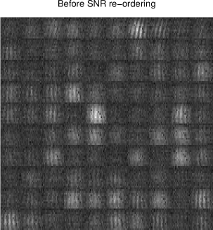
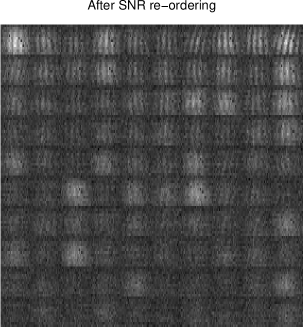
Figure 5: Left: sample of $100$ successive interferograms as recorded during the observation with two telescope of $ϵ~Sco$ in the low spectral resolution mode. Right: Re-ordering of this sample using the fringe SNR criterion (from left to right, bottom to top). Note that, some frames which are on the bottom of the right panel (that is with relatively low SNR) appear to be brighter than some above them (that is the flux is higher). However these frames do not exhibit fringes, which explains their positions.

5.2 Fringe criterion and fringe selection

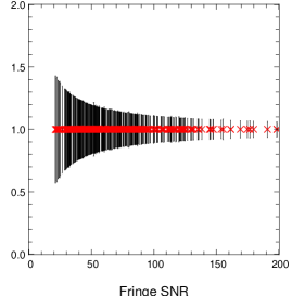
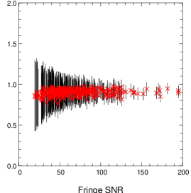
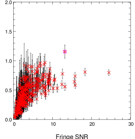
Figure 6: Visibility as a function of the fringe SNR criterion. Left: for jitter-free simulated data, using the real photometry observed on $ϵ~Sco$. The fringe contrast was set to $1$. Middle: Same as previous one, but atmospheric jitter attenuation has been added, corresponding to a integration time of $\tau=25\mathrm{ms}$. Right: Real $ϵ~Sco$ observation. The encircled data point on the plot, well above the other ones, is typical of a bad fit of the associated fringe, as explained in Section 5.1. Note that in the first two cases, the maximum of the fringe SNR is higher than in the real case. Indeed, in the simulated data, the noise on the coherent flux only arises from the photometry $P^{i}$ . In the real case, however it depends as well on the noise on the interferograms $i_{k}$ (see Eq. (19)).

For each frame of the set of data, Eq. (20) provides an estimation of the fringe Signal to Noise Ratio. As an example, Figure 5 presents $100$ fringes recorded on the detector during the 2-telescope observation of the calibrator $ϵ~Sco$ in July 2005, first in the order as they appeared during the observation and then after re-ordering them following the fringe criterion.

The aim of computing this criterion can be twofold: (i) during the observations, as mentioned in Section 3.4, it allows to detect the fringes and therefore to initiate the recording of the data only when it is meaningful and; (ii) calculated a posteriori during the data reduction phase, it enables to select the best frames (in terms of SNR) before estimating the observables. This second point is especially important where frames are recorded in presence of strong and variable fringe jitter.

In the ideal and unrealistic case where the fringes are not moving during the integration time, the fringe contrast is not attenuated by vibrations, and the frame by frame estimated visibility is constant, no matter the photometric flux level in each arm of the interferometer. As a result, the visibility as a function the function of the fringe SNR is constant, with the error bars increasing as the fringe SNR decreases. This is illustrated in Figure 6 (left). To obtain this set of jitter-free data, we have built interferograms using the carrying waves of the calibration matrix that simulate perfectly stable AMBER fringes. Then, we have added the photometry taken on the $ϵ~Sco$ data which allowed us to keep realistic photometric realizations taking into account the correct transmissions of the instrument. In that case, selecting the best fringes has no other ambition than improving the SNR on the observables by excluding the data with poor flux.

If the presence of atmospheric turbulence and without fringe tracker, the fringes are moving during the integration time, driving to lower the visibility. In average, the squared visibility is attenuated by a factor $\exp(-\sigma^{2}_{\phi^{p}_{hf}})$, where $\sigma^{2}_{\phi^{p}_{hf}}$ is the variance of the atmospheric high pass jitter, as explained in Section 3.6.2. The frame by frame visibility though, undergoes a random attenuation around this average loss of contrast. An example of the effect of the atmospheric jitter is given on Fig. 6 (middle), where previous set of simulated data has been used, with adding a frame by frame random attenuation taking into account the $\tau=25\mathrm{ms}$ integration time of the $ϵ~Sco$ observation. Once again, fringe selection only enables here to increase the SNR of the observables.

However, when we look at the real set of data obtained from the observation of $ϵ~Sco$, we obtain the plot displayed on Fig. 6 (right). The dispersion of the visibility, especially for low fringe SNR is unexpectedly large and can definitively not be explained by pure atmospheric OPD vibrations. As a matter of fact, these variations are due to the present strong vibrations along the VLTI instrumentation (adaptive optics, delay lines, $\ldots$), as this effect was previously revealed by the VINCI recombiner. These vibrations strongly reduce the fringe contrast and subsequently the value of the estimated visibilities, which explains the behavior of the visibilities as a function of the fringe SNR. Indeed, when the visibility tends toward $0$, because of severe jitter attenuation, the fringe criterion tends toward $0$ as well. On the contrary, the visibility plotted as a function of the fringe SNR saturates for high values of the latter.

The major issue is that such an effect is hardly calibratable because potentially non stationary. Hence, one convenient way to overcome the problem, beside increasing artificially the error bars to take into account this phenomena, is to only select the fringes which are the less affected by the vibrations, that is the fringes with the highest fringe SNR. One can then choose the percentage of selected frames from which the visibility will be estimated. The threshold must be chosen according to the following trade-off: reducing the number of accounted frames allows to get rid of most of the jitter attenuation, but, from a certain number – when the sample is not large enough to perform statistics –, it increases the noise on the visibility. Furthermore, it leads to mis-estimate the quadratic bias (see Eq. (25)), which is by essence a statistical quantity, and consequently drives to introduce a bias in the visibility.

Obviously, such a selection process must be handled with care, and its robustness with regard to the selection level has to be established for any given observation. In other words, for this method to be valid, the calibrated visibility expected value must remain the same, with only the error bars changing and eventually reaching a minimum at some specific selection level. In particular, this method seems well adapted above all to cases where the calibrator exhibits a magnitude close to the source’s one, where a similar behavior of the visibility distribution versus the SNR is expected. Going in further details of this point is nevertheless beyond the scope of this paper as it will be deeply developed in Millour et al. (2006). However note that we experimentally found this procedure to be generally robust, and that for typical observations performed until now with the VLTI, choosing $20\%$ of the frames as the final sample appeared to be a good compromise.

Note that, in order to produce the curve of Fig. 6, visibilities have been computed frame by frame (i.e. $M=1$). Thus, the semi-empirical calculation of the error bars given below in Section 5.3 does not work, and one has to use a full theoretical expression of the noise. From an analysis in the Fourier space, Petrov et al. (2003) showed that the theoretical error on the frame by frame visibility could be written:

$$\sigma^{2}(V^{ij})=\frac{n^{i}+n^{j}+N_{pix}\sigma^{2}}{n^{i}n^{j}}$$ (41)

where $n^{i}(t)=\sum_{k}^{N_{pix}}v_{k}^{i}P^{i}(t)$ is the total flux in the $i^{th}$ beam. This computation is not fully adapted to the AMBER data processing using $3$ telescopes since in that case the Fourier peaks are overlapping. Nevertheless, it gives a rough estimation of the noise level, within a factor of $2$, which is sufficient for the analysis discussed here.

Finally, despite that fringe selection has been performed to deal at best with the uncalibratable VLTI vibrations, the dispersion of the selected visibilities has still to be quadratically added to the error bar arising from the fundamental noises (as computed in section 5.3), in order to account for the reminiscent jitter attenuation, this latter having been reduced but not totally canceled out.

5.3 Visibilities and associated errors

Figure 7: Estimation of the raw squared visibility and its error-bars as a function of the wavelength for the observed calibrator $ϵ~Sco$, in low resolution mode. Visibility crosses and corresponding errors bars are computed thanks to Eq. (24) and Eq. (27) respectively. Circles and corresponding errors bars arise from bootstrapping technique. For sake of clarity, visibilities have been slightly shifted to the right and to the left of the corresponding wavelengths, respectively.

The raw squared visibility (that is biased by the atmosphere) and its associated error bar are estimated from the ensemble average of $M$ exposures, using Eq. (24) and (27) respectively. Figure 7 gives an example of the computed squared visibility in the low resolution mode, arising from the observation of the calibrator $ϵ~Sco$. For the example considered above, we find $V^{2}=0.2721\pm 0.0152$, after averaging the spectrally dispersed visibilities.

In order to validate the computation of the error bars, we use bootstrapping techniques (Efron & Tibshirani 1993). Such a method, by making sampling with replacement, constructs a large population of $N$ elements ($N$ estimated squared visibility) from the original measurements ($M$ coherent and photometric fluxes). If $N$ is large enough, the statistical parameters, that is the mean value and the dispersion of this population are converging respectively toward the expected value and the root mean square of the estimated parameters. $N$ being large enough, these quantities can be calculated by fitting a Gaussian distribution $p(V^{2})$ to the histogram of the bootstrapped population. Figure 8 give an example of the histogram and the resulting Gaussian fit. Using this method with $N=500$, we find for the same set of data $V^{2}=0.2719\pm 0.0149$, which is in excellent agreement with previous computation.

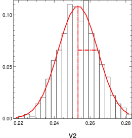
Figure 8: Histogram of the bootstrapped population of estimated squared visibilities for a given wavelength. The fit of this histogram by a Gaussian function is superimposed. The mean value and the root mean square of the Gaussian distribution gives the statistics of the estimated visibility.

Note that, although we observed this object in the low resolution mode, that at reasonably high flux, we find a relative error of the order of $6\%$. Such a quite large error bar is due to the atmospheric and intrumental jitter that, in the absence of fringe tracking, prevents to integrate time longer than a few tenth of milliseconds. When this latter device will be we expect to lower this error below the $1\%$ level, till $0.01\%$ for the brightest cases (assuming perfect fringe tracking, see Malbet et al. (1998); Petrov et al. (2006)). But it is not possible to achieve AMBER’s ultimate performances at that time.

5.4 Notion of instrumental contrast in AMBER

Given the calibration of the instrument described in Section 3.2 and its subsequent use for the estimation of the visibility in Section 3.5.1, the instrumental contrast of AMBER is self calibrated. In other words, the response of the AMBER/VLTI instrument to the observation of a point source – in absence of atmospheric turbulence – does not depend on the instrumental contrast but only on the visibility of the internal source (see. Eq. (24)). Thus, if one wants to characterize the instrumental contrast, that is the total loss of contrast due to the instrumentation, one needs to use another estimator in which the calibration part (the use of the knowledge of the instrument characteristics) is skipped. We thus can use the classical definition of contrast in the image plane, directly measured “by eyes” from the interferograms $i_{k}$, recorded pair by pair of telescopes (as for the computation of the carrying waves). In spatial coding, this can be done for each pixel of the interferogram. Using Eq. (3) and Eq. (10), it comes:

$$C_{r}^{ij}=C_{B}^{ij}\left(\frac{1}{N_{pix}}\sum_{k}\frac{2\sqrt{P^{i}v^{i}_{k}P^{j}v^{j}_{k}}}{P^{i}v^{i}_{k}+P^{j}v^{j}_{k}}\right)$$ (42)

Such an equation says that the instrumental contrast loss depends on two separate effects: (i) the polarization mismatch between the beams after the polarizers (vectorial effect) and; (ii) the misalignment of the interfering beams (taken into account in the product $v^{i}_{k}v^{j}_{k}$) together with the photometric unbalance between the two beams (scalar effect). Both effects are compensated when computing the visibility from the P2VM.

5.5 Closure phase

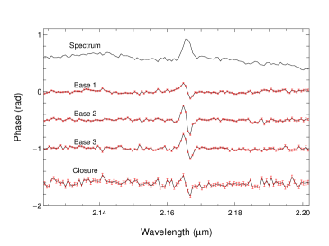
Figure 9: Example of differential phases and closure phase computation on an observed object with a rotating feature in the $\mathrm{Br}\gamma$ emission line ($α$ Arae, see Meilland et al. (2006) for a complete description and interpretation of these phases).

In the current situation, closure phases are computed using the estimator of Eq. (28), but a previous frame selection is performed before making the ensemble average of the bispectrum, because in all the data available there was a very low amount of frames which present simultaneously three fringe patterns. We have chosen an empirical selection criterion as the product of the three individual fringe SNR criteria (as defined by Eq. (20)). Closure phases internal error bars are computed statistically, taking the root mean square of all the individual frames divided by the square root of the number of frames (assuming statistical independence of the frames), since the tested theoretical error bars estimations does not give satisfactory results up to now.

An example of closure phase and closure phase error bars is given in the figure 9. The object is $α$ Arae which contains a rotating feature in the $\mathrm{Br}\gamma$ emission line (Meilland et al. 2006). A full description on how the closure phase and closure phase errors are computed will be part of the second paper on the AMBER data reduction (Millour et al. 2006).

5.6 Differential phase and piston

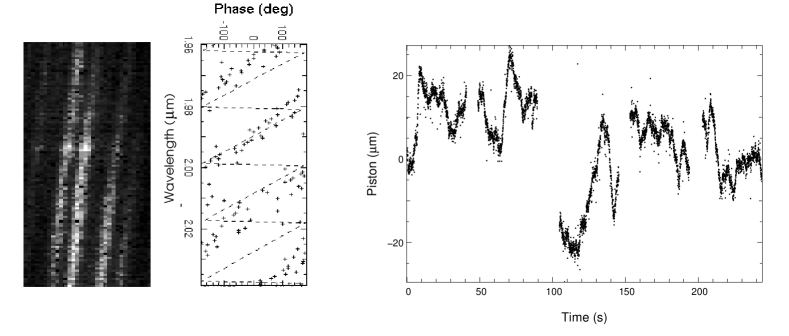
Figure 10: Piston estimation from the fringe pattern. From left to right is (i) the raw fringe pattern, the corresponding phase; (ii) the estimated linear component of the phase from the least square fit and; (iii) a piston time-sequence over $250$ seconds. Note that the piston rms is around $15\mu\mathrm{m}$, which is in agreement with the average atmospheric conditions recorded in Paranal (Martin et al. 2000).

An example of differential phases is given Figure 9. It is computed from the ensemble average of the cross spectrum as defined in the estimator of Eq. (30). Frame-by-frame correction of its linear part (i.e. unwrapping) has been performed. The resulting differential phase shows a typical rotation signal that is fully described in Meilland et al. (2006). Currently, as the closure phase, the internal error bars are computed statistically assuming that the differential phases are statistically independent frame to frame. An extensive description of the data processing and of the informations that can bring the differential phases will be described in our second paper (Millour et al. 2006) .

The computation of the linear component of the differential phase, that is the piston estimation is done on each spectral band separately (J, H or K), using the least square method described in Section 3.5.4. This algorithm has been extensively tested on the sky and validated as a part of the Observing Software of the AMBER instrument. An example of the fitting process as well as of the piston estimate is given in Figure 10.

6 Conclusions

We have described in this paper the data reduction formalism of the VLTI/AMBER instrument, that is the principles of the algorithm that lead to the computation of the AMBER observables. This innovative signal processing is performed in three main steps: (i) the calibration of the instrument which provides the calibration matrix that gives the linear relationship between the interferogram and the complex visibility; (ii) the inversion of the calibration matrix to obtain the so-called P2VM matrix then the complex visibility and; (iii) the estimation of the AMBER observables from the complex visibility, namely the squared visibility, the closure phase and the differential phase.

Note that this analysis requires that the calibration matrix must be both perfectly stable in time and very precise, that is recorded with a SNR much higher than the SNR of the interferograms. If the instrument is not stable between the calibration procedures and the observations, the P2VM will drift and as a result, the estimated observables will be biased. And if the calibration is not precise enough, it will be the limiting factor of the SNR of the observables. For the latter problem, it is thus recommended to set, during the calibration process, an integration time that insures a P2VM accuracy of at least a factor of $10$ higher than the accuracy expected on the measurements. To check the former problem of stability, it is advised to record one P2VM before and one P2VM directly after the observation. This procedure allows to quantify the drift of the instrument along the observations and to potentially reject the data is the drift appears to be too important. Note however that stability measurements in laboratory have shown the AMBER instrument to be generally stable at the hour scale at least.

Regarding the closure phase and the differential phase, we have produced here the theoretical estimators arising from the AMBER data reduction specific technique, as well as brief illustrations from real observations. A thorough analysis, that is practical issues and performances, of these two observables which deal the phase of the complex visibility will be given in a forthcoming paper (Millour et al. 2006)

For the squared visibility, we have defined an estimator that is self-calibrated from the instrumental contrast, and we have investigated its biases. The quadratic bias, which is an additive quantity and results in the quadratic estimation in presence of zero-mean value additive noise, can be easily corrected, providing the computation of the error of the fringe measurements. Atmospheric and instrumental biases, which attenuate in a multiplicative manner the visibility, come respectively from the high frequency fringe motion during the integration time – namely the jitter –, and from the loss of spectral coherence when the fringes are not centered at the zero optical path difference – that is the atmospheric differential piston. The latter can be estimated from the differential phase and its consecutive attenuation can be corrected knowing the shape of the spectral filter and the resolution of the spectrograph. The former, when strictly arising from atmospheric turbulence, can be calibrated by a reference source, providing it has been observed shortly before/after the object of interest. When instrumental, hardly calibratable vibrations add themselves in the jitter phenomenon, as it is presently the case for the VLTI, we propose a method based on sample selection that allows to reduce the attenuation and the associated dispersion on the visibilities.

However at this point, because of the presence of these instrumental vibrations, and because of the absence of the FINITO fringe tracker as well, it is neither possible to develop optimized tool to identify and calibrate the biases coming from the atmospheric turbulence, nor to present an analysis of the ultimate performances of the VLTI/AMBER instrument. These points will be developed in our next paper on the AMBER data reduction methods, once the problems mentioned above, which are independent of the AMBER instrument, will have been resolved.