Hard TeV spectra of blazars and the constraints to the IR intergalactic background

Abstract

Recent gamma–ray observations of the blazar 1ES 1101–232 (redshift $z=0.186$) reveal that the unabsorbed TeV spectrum is hard, with spectral index $\alpha\lesssim 0.5$ [$F(\nu)\propto\nu^{-\alpha}$]. We show that simple one–zone synchrotron self–Compton model can explain such hard spectra if we assume a power law energy distribution of the emitting electrons with a relatively high minimum energy. In this case the intrinsic TeV spectrum can be as hard as $F(\nu)\propto\nu^{1/3}$, while the predicted X–ray spectrum can still be much softer. The observations of 1ES 1101–232 can therefore be reconciled with relatively high intensities of the infrared background, even if some extreme background levels can indeed be excluded. We show that the other TeV sources (Mrk 421, Mrk 501 & PKS 2155–304) can be interpreted in the same framework, with a somewhat larger minimum energy.

1 Introduction

The intrinsic high-energy emission from extragalactic sources is attenuated by the pair-production process (Nishikov 1962, Gould 1966, Stecker et al. 1992). Photons in the TeV range ($\epsilon_{\gamma}$) interact with low–energy photons from the extragalactic infrared background ($\epsilon_{\rm IR}$) and produce electron–positron pairs ($\epsilon_{\rm IR}+\epsilon_{\gamma}\rightarrow e^{+}e^{-}$). The total absorption depends on the history of the reaction rate along the line–of–sight, and therefore, on the distance travelled and on the local density of the low-energy target photon field, both a function of redshift $z$. This process will affect the high–energy TeV end of the observed blazar spectra. Since the optical depth depends strongly on the incident TeV–photon energy the process leads to a steepening of the observed spectrum with respect to the intrinsic (unabsorbed) one.

Thus, the observed spectra from distant blazars contain information on both the IR background radiation field history and the intrinsic properties of the source. From the viewpoint of blazar studies the latter is just an undesirable extrinsic effect that must be corrected for. In contrast, from the opposite perspective, it allows the measurement of the IR background. In both cases these two independent processes have to be disentangled by either modeling both simultaneously (e.g. De Jager & Stecker 2002, Kneiske et al. 2004), or measuring one independently (see Hauser & Dwek 2001 for a review).

Unfortunately it proved very difficult to constrain the IR background independently, and different groups tried to constrain models for the IR background from TeV observations assuming that the blazar spectrum is a well-behaved power–law (e.g. Costamante et al. 2003, Dwek & Krennrich 2005). The best perspective for such studies is offered by high–redshift blazars, since the absorption will be strong. Recently, Aharonian et al. (2006) presented a study along these lines, based on the TeV spectra of high–redshift blazars recently measured by the H.E.S.S. instrument. They de–reddened the observed TeV data of 1ES 1101-232 with different models of the IR backgrounds, and concluded that the resulting intrinsic spectrum is always very hard. The index of the intrinsic spectrum should be equal to $\alpha=0.5$ if the level of the IR background is close to the absolute lower limit obtained from direct integration of the light from resolved galaxies (Madau & Pozzetti, 2000). Larger IR background levels should correspond to intrinsic TeV spectra harder than $\alpha=0.5$. Note that this spectral index is already harder than the spectral index observed in other nearby TeV sources and that the difference will be more important for larger background levels. Aharonian et al. (2006) also commented on the theoretical difficulties to explain spectra harder than $\alpha=0.5$, which would imply quite unexpected physics. These facts led Aharonian et al. (2006) to prefer the solution of minimal IR background.

In this paper we show instead that spectra harder than $\alpha=0.5$ can be obtained in “normal” one–zone homogeneous synchrotron self–Compton (SSC) models, as long as there is a deficit of low energy electrons with respect to the extrapolation from higher energies. This can be achieved by assuming an emitting particle distribution which is a double power law, with a flat slope ($<2$) of the first, low energy portion, or assuming a simple power law, but with a relatively high low energy cut–off. In these cases the limits on how hard a TeV spectrum can be is $\alpha=-1/3$, while well accounting for a much softer X–ray spectrum.

We discuss this result with the aim of finding limits on the IR background and also in the context of explaining the other TeV sources (with a softer intrinsic spectrum) with the same model.

2 SSC models

The simplest possible scenario able to explain the X–ray and TeV emission of a blazar assumes a homogeneous, spherical source filled by tangled magnetic field and relativistic electrons.

Since in TeV blazars we must have electrons of very large energies, the scattering process occurs partly in the Klein–Nishina regime. In this regime the scattering process becomes inefficient, and for typical electron distributions the SSC process can be well described by approximating the scattering cross section with a step function, equal to the Thomson cross section for incident photon energies $h\nu<m_{\rm e}c^{2}/\gamma$, and zero otherwise. This means that electrons of increasingly large energies scatter an increasingly smaller fraction of synchrotron seed photons, steepening the resulting SSC spectrum with respect to the “canonical” value of $\alpha=(n-1)/2$. Note that this steepening introduced by the Klein–Nishina effects is virtually inescapable, since the scattering occurs completely in the Thomson limit only for extremely large values of the beaming factor: $\delta>1000$ (see e.g. Katarzynski et al. 2005a). In the next section we will find what is the high energy spectral index corresponding to a given particle energy distribution, assuming “usual” parameters for our TeV source, namely: source radius $R=10^{15\to 16}$ [cm], magnetic field intensity $B=1\to 0.01$ [G], Doppler factor $\delta=10\to 50$ and approximating the particle energy distribution by a broken power law with the index $n_{1}$ [$N(\gamma)=K\gamma^{-n_{1}}$] below the break energy ($\gamma_{\rm brk}$) and $n_{2}$ above the break [$N(\gamma)=K\gamma_{\rm brk}^{n_{2}-n_{1}}\gamma^{-n_{2}}$], where $K$ is the density of the particles with $\gamma=1$. If the minimal $\gamma$ is greater than unity ($\gamma_{\rm min}>1$) the density of the particles with minimum energy ($K^{\prime}$) is given by $K^{\prime}=K\gamma_{\rm min}^{-n_{1}}$.

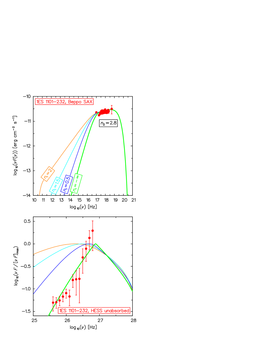
Figure 1: Synchrotron emission (upper panel) and self–Compton radiation (lower panel) for different values of $n_{1}$. The green spectra, generated by the truncated single power law particle energy spectrum ($n_{1}=-\infty$), provide the best fit for observations of 1ES 1101–232 made by $Beppo$SAX (Wolter et al. 2002) and H.E.S.S. (Aharonian et al. 2006). Note that the spectra on the lower panel have been normalized to the peak level and the H.E.S.S. observations has been unabsorbed according to the model proposed by Kneiske et al. (2004).

2.1 Flat electron distributions

A flat slope of the electron distribution ($n_{1}<2$) may help to explain the intrinsic TeV spectrum of 1ES 1101–232. Assuming the lowest possible absorption level, Aharonian et al. (2006) have estimated the intrinsic spectral index $\alpha\simeq 0.5$ for this particular source. We verified that it is roughly possible to reproduce such a spectrum if we assume that $n_{1}\simeq 1.5$ (note that in the Thomson limit $\alpha=0.5$ would correspond to $n_{1}=2$.). In this case, however, we do not obtain a power law intrinsic TeV spectrum. The spectrum is curved, with $\alpha$ changing from $\alpha=0.25$ in the GeV range to $\alpha=1$ at the peak of the emission at a few TeV.

Since $n_{1}\simeq 1.5$ can explain the spectrum derived for the minimal IR background case, we then ask if a smaller value of $n_{1}$, producing an harder spectrum, can allow for a larger level of the IR background. In Fig. 1 we show different synchrotron and inverse–Compton spectra for different $n_{1}$ indices. The spectral index of the first part of the thin synchrotron emission ($\alpha_{1}$) depends directly on $n_{1}$ [$\alpha_{1}=(n_{1}-1)/2$] down to the limiting value $n_{1}=1/3$. Below this limit the index remains constant $\alpha_{1}=-1/3$. This is due the fact that, below the limit, the dominant part of the low frequency emission is generated by electrons with $\gamma\simeq\gamma_{\rm brk}$. Therefore, the spectrum in the discussed range is equivalent to the spectrum produced by a monoenergetic population of electrons, which can be approximated by a power law with $\alpha=-1/3$ below the maximum of the emission (e.g. Rybicki & Lightman 1979). This means that even in the extreme case of the truncated, single power law energy distribution ($n_{1}=-\infty$) there is always a “source” of low energy photons due to the low frequency emission ($F_{\rm syn}\sim\nu^{1/3}$) of the high energy electrons ($\gamma\simeq\gamma_{\rm brk}$). The spectral index of the inverse–Compton emission in the Thompson regime is equivalent to the index of the target radiation field (e.g. Rybicki & Lightman 1979). Since $\alpha_{1}$ is limited to –1/3 also the index of the inverse–Compton emission below the peak is limited to this value. Moreover, this index does not depend on $n_{2}$. The index of the inverse–Compton emission above the peak is given by $\alpha=2\alpha_{2}-\alpha_{1}$, where $\alpha_{1}=-1/3$. This relationship can be easily derived from the approximation of the scattering derived by Tavecchio et al. (1998).

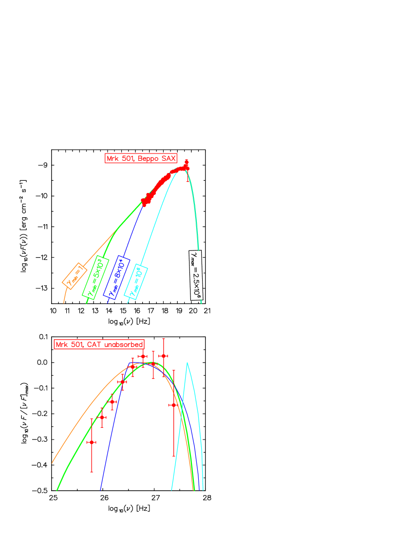
Figure 2: Synchrotron emission (upper panel) and the self–Compton radiation (lower panel) for different values of the $\gamma_{\rm min}$ parameter. The best fit for the $Beppo$SAX (Pian et al. 1998) and CAT (Djannati-Atai et al. 1999) observations of Mrk 501 is indicated by the green lines. Note that the inverse–Compton spectra have been normalized and the TeV observations have been unabsorbed according to the model proposed by Kneiske et al. (2004).

To directly check the applicability of the SSC scenario that assumes $n_{1}<2$ we have applied our computations to the emission of 1ES 1101–232 observed by $Beppo$SAX (Wolter et al., 2000) and H.E.S.S. (Aharonian et al., 2006) experiments. The TeV data (here and in all the other cases in the following) have been unabsorbed according to the “best-fit” model proposed recently by Kneiske et al. (2004). The predictions of this model are also consistent with those of the model proposed by Stecker et al. (2005). The model provides a significantly stronger absorption level than the minimal possible absorption suggested by Aharonian et al. (2006). However, our best fit for the expected intrinsic spectrum, in a framework of the above mentioned SSC scenario, has been obtained for the limiting case ($n_{1}=-\infty$). This indicates that the absorption is close to the highest possible value that can be accommodated by this scenario. If the absorption is stronger, as suggested by some models (e.g. De Jager & Stecker 2002), then our SSC scenario cannot explain the intrinsic TeV emission of 1ES 1101–232. The detailed values of the physical parameters used in our computations are discussed in the last section of this work, where we apply this scenario also to other sources.

The truncated particle energy distribution corresponds to the limit $n_{1}\rightarrow-\infty$ of a broken power law. For clarity, we will refer in the following to the break energy as $\gamma_{\rm min}$. For such a electron distribution, the shape of the TeV emission depends strongly on $\gamma_{\rm min}$, and we will therefore investigate this is some detail.

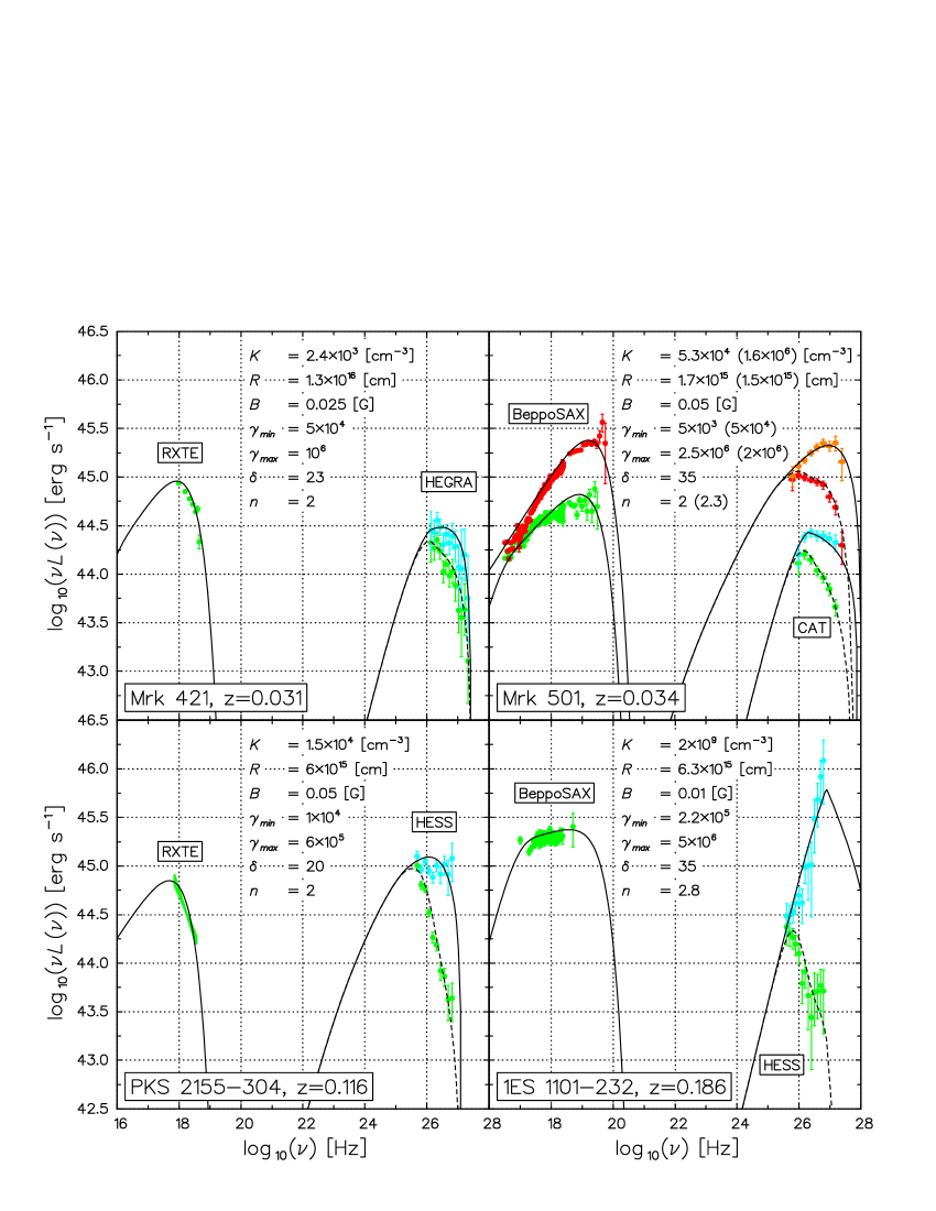
Figure 3: X–ray and TeV emission of four TeV blazars located at different redshifts. For all the sources we have applied the same SSC scenario, assuming that the emitting electrons are distributed in energy as a single power law with a low energy cut-off at $\gamma_{\rm min}$. All the TeV spectra have been unabsorbed according to the model of Kneiske et al. (2004). Solid lines are the best fits for the expected intrinsic emission whereas dashed lines indicate the observed spectra. For an easier comparison of the different sources, we transformed the observed flux in luminosity.

2.2 Changing $\gamma_{\rm min}$

As we have shown in the previous subsection a particle distribution with a low energy cut-off provides the best explanation for the emission of 1ES 1101–232. We here show the effects of changing the value of the low energy cut–off, which we will call $\gamma_{\rm min}$. The result of our calculations is shown in Fig. 2. We have applied this test for the $Beppo$SAX (Pian et al., 1998) and CAT (Djannati-Atai et al., 1999) observations of Mrk 501 from 16^th April, 1997.

For this test, we fix the slope of the particle distribution to $n=2$, which provides the best fit for the used X–ray observations of Mrk 501. In the first approach we assume the minimal possible value of $\gamma_{\rm min}=1$. This means that the model is equivalent to the standard SSC scenario and is providing a relatively broad peak for the inverse–Compton emission. Nevertheless, this approach is able to roughly explain the unabsorbed TeV spectrum. However, the increase of the $\gamma_{\rm min}$ value by about three orders of magnitude provides a slightly narrower peak and therefore better explanation for the spectrum. A value of $\gamma_{\rm min}$ greater by one more order of magnitude is the limiting value if we want to explain the entire X–ray spectrum. However, this already high value of $\gamma_{\rm min}$ is drastically modifying the TeV spectrum, where the limiting slope ($\alpha=-1/3$) of the emission becomes well visible (blue line in Fig. 2). Finally, a quasi–monoenergetic electron distribution cannot explain the X–ray nor the TeV emission. Note that for values of $\gamma_{\rm max}$ close to $\gamma_{\rm min}$, the second part of the TeV spectrum, above the peak, is curved and it is not a power law.

3 Application to other TeV blazars

We have already applied our specific SSC scenario to 1ES 1101–232 and Mrk 501. In this section we apply this model to two other TeV sources, Mrk 421 and PKS 2155–304, and compare the results.

The RXTE and HEGRA observations of Mrk 421 (Krawczynski et al., 2001) can be fitted assuming that the X–ray emission is done by the exponential synchrotron tail of the highest energy particles at $\gamma_{\rm max}$. Therefore, the index of the particle energy spectrum and $\gamma_{\rm min}$ are not constrained by the data. The same approach can explain the RXTE and H.E.S.S. observations of PKS 2155–304 (Aharonian et al., 2005). Note that it is also possible to explain these observations, as well as the observations of Mrk 501, assuming $\gamma_{\rm min}\simeq 1$. We performed our computations to show that the assumption of having $\gamma_{\rm min}\gg 1$ (required to explain the emission for 1ES 1101–232), works very well also for other sources. In Fig. 3 we show the results of our modeling and give the values of the input parameters. Note that for Mrk 501 we provide also the spectral fits for the observations made on April 7^th, 1997. Moreover, in the case of Mrk 421, Mrk 501 and PKS 2155–304 the X-ray and TeV observations were made almost simultaneously, whereas for 1ES 1101–232 we use the X–ray spectrum from January 1997 and the TeV data collected over March-June 2004-2005.

Note that the value of the magnetic field used in our calculations is significantly smaller that the value estimated from the equipartition between the magnetic field energy density and the electron energy density.

4 Discussion

We have shown that the standard SSC model can explain the specific observations of the relatively distant TeV blazar 1ES 1101–232. Assuming a truncated power law energy distribution, with $\gamma_{\rm min}\gg 1$, we can well explain the intrinsic TeV spectrum even assuming a stronger absorption than the upper limit suggested by Aharonian et al. (2006). This assumption appears in very good agreement with the recent estimates of the IR intergalactic background (Kneiske et al. 2004, Stecker et al. 2005). The limit on how hard an SSC spectrum can be is $\alpha=-1/3$. This limit in turn translates in a limit on the amount of absorption suffered by TeV photons, and hence on the level of the IR background.

Concerning the reason of having $\gamma_{\rm min}\gg 1$, we can propose two answers. The first is the injection of an already truncated power law spectrum from a shock region. If, in addition, the cooling process is inefficient for the the particles at lower energies (close to $\gamma_{\rm min}$), the particle distribution will not develop a low energy tail in a “reasonable” time, namely a dynamical time, over which we can assume that the physical conditions (size, densities, magnetic field) are constant (since the source has bulk motion, after a dynamical time it will be located in a larger part of the jet, and not contribute any longer to the observed flux). Note that in our particular simulations also particles with $\gamma\simeq\gamma_{\rm max}$ are not affected by the cooling in one crossing time ($R/c$).

In a second, more complex, scenario all particles are accelerated efficiently at the shock front almost up to some maximal energy. Then they escape downstream of the shock and cool. However, the cooling process may be compensated (at least in part) by some stochastic turbulent acceleration (Katarzynski et al., 2005b). The competition between re-acceleration (heating) and cooling may single out an equilibrium energy where the two processes balance. This equilibrium energy may correspond to the $\gamma_{\rm min}$ assumed in our simple SSC scenario.

The changes of $\gamma_{\rm min}$ and $\gamma_{\rm max}$ may have various impacts for the source variability, especially for the correlation between the X–ray and TeV emission. As an example, when $n_{2}<3$ and $\gamma_{\rm min}\ll\gamma_{\rm max}$ the change of $\gamma_{\rm min}$ may not affect the X–ray emission while having a strong impact for the TeV radiation. Such a scenario could explain the orphan TeV flare in 1ES 1959+650 (Krawczynski et al., 2004). On the contrary, a change of $\gamma_{\rm max}$ would produce a significant X–ray variability without any change in the TeV flux below the TeV peak.

References

- Aharonian et al. (2005) Aharonian F., Akhperjanian A.G., Bazer–Bachi A.R., et al. 2005, A&A, 442, 895
- Aharonian et al. (2006) Aharonian F., Akhperjanian A.G., Bazer–Bachi A.R., et al. 2006, Nat, in press (astro-ph/0508073)
- Costamante et al. (2003) Costamante L., Aharonian F., Ghisellini G. & Horns D. 2003, New Astron. Rev., 47, 677
- De Jager & Stecker (2002) De Jager O.C., & Stecker F.W. 2002, 566, 738
- Djannati-Atai et al. (1999) Djannati–Atai A., Piron F., Barrau A., et al., 1999, AA, 350, 17
- Dwek & Krennrich (2005) Dwek E. & Krennrich F., 2005, ApJ, 618, 657
- Gould (1966) Gould R. J., Schreder G. P., 1966, Phys. Rev. Lett. 16, 252
- Hauser & Dwek (2001) Hauser M. G., Dwek E., 2001, ARA&A, 39, 249
- Katarzynski et al. (2005a) Katarzynski K., Ghisellini G., Tavecchio F., Maraschi L., Fossati G. & Mastichiadis A. 2005a, A&A, 433, 479
- Katarzynski et al. (2005b) Katarzynski K., Ghisellini G., Mastichiadis A., Tavecchio F. & Maraschi L. 2005b, A&A, in press
- Kneiske et al. (2004) Kneiske T.M., Bretz T., Mannheim K., & Hartmann D. H., 2004, A&A, 413, 807
- Krawczynski et al. (2001) Krawczynski H., Sambruna R., Kohnle A., et al., 2001, ApJ, 559, 187
- Krawczynski et al. (2004) Krawczynski H., Hughes S.B., Horan D., et al. 2004, ApJ, 601, 151
- Madau & Pozzetti (2000) Madau P. & Pozzetti L., 2000, MNRAS, 312, L9
- Nishikov (1962) Nishikov A. I., 1962, Sov. Phys. JETP, 14, 393
- Pian et al. (1998) Pian E., Vacanti G., Tagliaferri G., et al., 1998, ApJ , 492, L17
- Rybicki & Lightman (1979) Rybicki G. & Lightman A.P., 1979, Radiative Processes in Astrophysics, Wiley Interscience, New York
- Stecker et al. (1992) Stecker F. W., de Jager O.C. & Salamon M. H., 1992, ApJ, 390, L49
- Stecker et al. (2005) Stecker F. W., Malkan, M. A. & Scully, S. T., 2005, ApJ, submitted, (astro-ph/0510449)
- Tavecchio et al. (1998) Tavecchio F., Maraschi L. & Ghisellini G., 1998, ApJ , 509, 608
- Wolter et al. (2000) Wolter A., Tavecchio F., Caccianiga A. & Tagliaferri G., 2000, A&A, 357, 429