Spectral and Fourier analyses of X-ray quasi-periodic oscillations in accreting black holes

Abstract

We study energy dependencies of quasi-periodic oscillations from a number of black hole X-ray binaries. The selected sources were observed by RXTE at time periods close to state transitions and showed QPO in the 1–10 Hz range. We have constructed QPO root-mean-square energy spectra, which provide information about underlying physical process leading to QPO generation. These spectra show an interesting anti-correlation with the time averaged spectra. The QPO r.m.s. spectra are harder than the time averaged spectra when the latter are soft, while they are softer than the time averaged spectra when the latter are hard. We then discuss these observational results in the context of simple spectral variability models. Hard QPO spectra can be produced by quasi-periodic modulations of the heating rate of the Comptonizing plasma, while soft QPO spectra result from modulations of the cooling rate by soft photons.

1 Introduction

A common feature in X-ray power spectra from many X-ray binaries (XRB) are quasi-periodic oscillations (QPO). Many “flavours” of QPO have been identified, with some correlations between their frequencies (Psaltis, Belloni & van der Klis 1999). For example, low frequency ($f$ of a few Hz) QPO in black hole XRB seem to appear preferentially when the state of the source changes (Rutledge et al. 1999). They are mostly observed in luminous states, high or very high state, when the energy spectrum is rather complex, showing both disc thermal component and high energy Comptonized component (see QPO observations review in Wijnands 2001). Models of QPO so far concentrated on identifying the frequencies of oscillations, with very little if any attention paid to the fact that it is the hard X–rays which are modulated (see QPO models review in Psaltis 2001). The results of Gilfanov, Revnivtsev & Molkov (2003) and Revnivtsev & Gilfanov (2005) are perhaps the only ones where the energy spectra of QPO are discussed and interpreted. These authors applied Fourier frequency resolved spectroscopy (Revnivtsev, Gilfanov & Churazov 1999, 2001) to show in particular that the kilo-Hz QPO spectra in neutron star XRB are the same as spectra at other Fourier frequencies. This can be interpreted as common spatial origin of the X-rays showing the usual broad band noise variability and the more coherent quasi-periodic variability. The spectral shape of these components is consistent with Comptonized emission from a boundary layer.

Fourier spectroscopy techniques are particularly suitable for analysis of QPO. However, the approach of Revnivtsev et al. (1999) requires integrating the power density spectra over a narrow frequency interval around a chosen frequency resulting in contamination of the Fourier frequency resolved spectrum of the QPO by a contribution from the broad band variability component. Thus, in this paper we construct a root-mean-square spectrum, where each point is the r.m.s.  variability integrated over the component (e.g. a Lorentzian) describing the QPO in the broad band power spectrum. Such energy dependences of QPO amplitude in XRB has been investigated before (e.g. Belloni et al. 1997; Cui et al. 1999; Rao et al. 2000; Tomsick & Kaaret 2001; Rodriguez et al. 2004; Casella et al. 2004; see review in van der Klis 2006). The main conclusion from these studies is that the QPO amplitude increases with energy up to at least $\sim 20$ keV. This suggests immediately that the oscillations are connected with the high energy spectral component, rather than with the disk component.

Table 1: Log of RXTE observations

Object	MJDa	yymmdd	Observation ID	Spectral state
XTE J1859+226 (I)	51463.8	991012	40124-01-05-00	soft state at the luminosity peak1
XTE J1859+226 (II)	51465.9	991014	40124-01-10-00	”
XTE J1859+226 (III)	51472.5	991021	40124-01-21-00	”
XTE J1859+226 (IV)	51474.8	991023	40124-01-25-00	”
GRS 1915+105 (I)	50422.0	961204	20402-01-05-00	C state (class $\chi$)2
GRS 1915+105 (II)	52768.6	030509	80127-03-01-00	” 3
GRS 1915+105 (III)	52731.5	030402	80127-01-03-00	”
XTE J1550-564 (I)	51068.3	980912	30188-06-05-00	soft state4
XTE J1550-564 (II)	51245.4	990308	40401-01-53-00	,,anomalous” state5
XTE J1550-564 (III)	51248.1	990311	40401-01-51-01	”
XTE J1550-564 (IV)	51250.7	990313	40401-01-57-00	”
XTE J1550-564 (V)	51683.8	000519	50135-01-03-00	hard state6
4U 1630-47 (I)	50853.1	980209	30178-01-01-00	hard state7
4U 1630-47 (II)	50853.7	980209	30178-01-02-00	”

^a Start of observation, ${\rm MJD}={\rm JD}-{\rm 2,400,000.5}$
References to papers with spectral/timing analysis:
¹ Casella et al. (2004)
² Sobolewska & Życki (2003)
³ Rodriguez et al. (2004)
⁴ Sobczak et al. (2000)
⁵ Remillard et al. (2002), Kubota & Done (2004)
⁶ Tomsick et al. (2001), Rodriguez et al. (2003)
⁷ Dieters et al. (2000)

The significance of the r.m.s. energy spectrum is that it describes the energy spectrum of the process responsible for a given variability component (e.g. a QPO), if the variability is generated by fluctuactions of the normalization of a separate spectral component (Gilfanov et al. 2003; Życki & Sobolewska 2005, hereafter Paper I). If the QPO is produced by an additional modulation of one or more physical parameters determining the spectrum, its r.m.s. spectrum has less direct interpretation, but still it contains the signatures of the modulation (Paper I). Energy dependencies of r.m.s. spectra were investigated by many authors with a goal of determining how the spectral components vary with respect to each other. Recently, Gierliński & Zdziarski (2005) investigated the r.m.s. energy spectra of a number of XRBs in various spectral stated and interpreted them in terms of variations of plasma heating/cooling rate in a scenario where the time average energy spectrum consists of a disc blackbody and a hybrid (thermal/non-thermal) Comptonization. However, their r.m.s. spectra were averaged over all variability components (Fourier frequency).

In this paper we perform a systematic study of energy dependencies of low-frequency QPO in black hole XRB in different spectral states. We analyse RXTE data from a number of sources observed at time periods close to or during state transitions, when the sources showed QPO in 1–10 Hz range. We selected data with good energy and time resolutions, enabling construction of power density spectra (PDS) in at least 12 energy channels covering the 3–40 keV range. We then constructed the r.m.s. spectra of the QPO and compared them with the mean energy spectra. Finally, we compared the results of data analysis with the predictions of theoretical models. The models themselves are described in detail in Paper I.

Table 2: Fits to time averaged spectra

	diskbb/thComp 1			thComp 2
Dataset	$kT_{\rm bb}$ (keV)	$\Gamma$	$kT_{\rm e}$ (keV)	$\Gamma$	$kT_{\rm e}$ (keV)	$R$	$\xi$	$\chi^{2}/{\rm dof}$
XTE J1859+226 (I)a	$0.70^{+0.09}_{-0.16}$	–	–	$2.19\pm 0.08$	$44^{+100}_{-18}$	$0.19^{+0.13}_{-0.10}$	$185^{+4700}_{-110}$	73.9/69
XTE J1859+226 (II)a	$0.81\pm 0.04$	–	–	$2.38\pm 0.03$	150(f)	$0.15^{+0.07}_{-0.03}$	$(4.4^{+9.6}_{-3.9})\times 10^{3}$	61.2/67
XTE J1859+226 (III)a	$0.82\pm 0.03$	–	–	$2.37\pm 0.02$	150(f)	$0.16\pm 0.03$	$(2.5^{+5.5}_{-1.6})\times 10^{3}$	74.6/70
XTE J1859+226 (IV)a	$0.83\pm 0.03$	–	–	$2.34\pm 0.02$	150(f)	$0.16^{+0.06}_{-0.02}$	$(2.9^{+6.0}_{-2.0})\times 10^{3}$	80.5/70
XTE J1550-564 (I)c	$0.64^{+0.06}_{-0.20}$	$1.98\pm 0.12$	$7.5^{+1.2}_{-0.9}$	$2.23^{+0.10}_{-0.37}$	150 (f)	$0.43^{+3.2}_{-0.15}$	$(15^{+25}_{-10})\times 10^{3}$	58.2/70
XTE J1550-564 (II)c	$0.92\pm 0.02$	$2.86^{+0.24}_{-0.19}$	$17^{+51}_{-12}$	$1.88\pm 0.20$	150(f)	$>0.8$	$(2.1^{+4.0}_{-1.7}\times 10^{3}$	63.5/69
XTE J1550-564 (III)b	$0.66\pm 0.01$	$4.51\pm 0.17$	100(f)	$2.19\pm 0.05$	150(f)	$0.40^{+0.33}_{-0.08}$	$(4.4^{+15.6}_{-3.6})\times 10^{3}$	51.2/73
XTE J1550-564 (IV)b	$0.47\pm 0.03$	$4.1\pm 0.4$	100(f)	$2.21\pm 0.04$	150(f)	$0.29^{+0.34}_{-0.04}$	$(1.2^{+7.8}_{-1.0})\times 10^{3}$	74.5/74
GRS 1915+105 (I)a	$0.58^{+0.13}_{-0.08}$	–	–	$2.29\pm 0.07$	$40^{+29}_{-20}$	$0.47^{+0.73}_{-0.20}$	$(2.0^{+4.0}_{-1.7})\times 10^{4}$	59.7/71
GRS 1915+105 (II)c	$0.19^{+0.13}_{-0.19}$	$2.21^{+0.07}_{-0.05}$	$5.1^{+0.4}_{-0.9}$	$2.25^{+0.09}_{-0.32}$	$>25$	$1.7^{+1.7}_{-1.1}$	$(7.3^{+10}_{-4.6})\times 10^{4}$	69.2/62
GRS 1915+105 (III)c	$1.02^{+0.24}_{-0.17}$	$2.18^{+0.16}_{-0.50}$	$4.1^{+0.4}_{-0.6}$	$2.50^{+0.40}_{-0.25}$	150(f)	$>0.25$	$(3.5^{+3.7}_{-2.1}\times 10^{4}$	44.5/65
4U 1630-47 (I)a	$1.06^{+0.18}_{-0.30}$	–	–	$1.98^{+0.02}_{-0.04}$	$>45$	$0.10^{+0.06}_{-0.02}$	$(4.9^{+8.1}_{-4.5})\times 10^{3}$	80.9/73
4U 1630-47 (II)a	$1.05^{+0.22}_{-0.18}$	–	–	$1.98\pm 0.04$	$37^{+40}_{-15}$	$0.07^{+0.10}_{-0.01}$	$(1.8^{+6.0}_{-1.6})\times 10^{3}$	44.7/66
XTE J1550-564 (V)a	$0.88^{+0.11}_{-0.09}$	–	–	$1.677^{+0.019}_{-0.010}$	$>64$	$0.11\pm 0.03$	$(1.7^{+5.0}_{-1.1})\times 10^{3}$	41.8/69

^a Model: diskbb + thComp
^b Model: thComp + thComp
^c Model: diskbb + thComp + thComp
(f) Parameter was fixed

2 Data selection and description of time-averaged spectra

We made use of the RXTE archive data. We were particularly interested in observations during which a pronounced (rms $>$ 10%) and coherent 1–10 Hz QPO were present in the power density spectrum. A basic criterion was good timing and spectral resolution of the data. The log of all observations is presented in Table 1.

We extracted Standard 2 PCA spectra from top and mid layer from all available units. Standard selection criteria and dead time correction procedures were applied. The PCA background was estimated using the pcabackest package (ver. 3.0), while the response matrices were made for each observation with pcarsp ver. 10.1 tool. Systematic error of 0.5 per cent were added to each bin of PCA spectra, to take into account possible calibration uncertainties. HEXTE data (Archive mode, Cluster 0) were extracted using the same selection criteria as those for the PCA. Background was estimated using hxtback tool. For spectral modelling we used the PCA data in 3–20 keV range and HEXTE data 20–200 keV range.

The spectral model consisted of a disc blackbody and thermal Comptonization components, modified by photoelectric absorption. For Comptonization we use the thComp XSPEC model (Zdziarski, Johnson & Magdziarz 1996). This is parametrized by the asymptotic spectral index, $\Gamma$, seed photon temperature, $T_{0}$, and electron temperature, $kT_{\rm e}$. Disc blackbody (maximum) temperature is denoted $T_{\rm bb}$. In most cases we assume $T_{0}=T_{\rm bb}$ as can be expected, if it is the disc photons which are Comptonized, but we will also consider cases where the temperatures are de-coupled. The thComp model computes also self-consistently the reprocessed component consisting of the Compton reflected continuum and the Fe fluorescent K$\alpha$ line (Życki, Done & Smith 1999 and references therein). The main parameters here are the relative amplitude of the component, $R$, ionization parameter of the reprocessor, $\xi$, and the inner disc radius used for computing the smearing of spectral features due to relativistic effects, $R_{\rm in}$.

Results of the fits to the time averaged spectra are given in Table 2 and described in detail in following Sections. All uncertainties in the Table are 90% confidence limits for one parameter of interest, i.e. $\Delta\chi^{2}=2.71$. We allowed for a free normalization between the data from PCA and HEXTE.

2.1 XTE J1859+226

We study four observations of the X-ray nova XTE J1859+226 at the luminosity peak during its 1999 outburst. Detailed timing analysis and identification of different types of QPO was presented in Casella et al. (2004). During the observations the source was in a very high state. The data are well described with a disc blackbody model with a temperature of $\sim 0.7$–0.8 keV and its thermal Comptonization on electrons with temperature fixed at $kT_{\rm e}=150$ keV (lower temperature, $kT_{\rm e}\approx 40$ keV is required for the first observation). The Comptonized continuum has a photon index of $\Gamma=2.1$– 2.4. In all datasets a weak (amplitude $R=0.1$–0.2), highly ionized (ionization parameter $\xi=1200$–2700) reflection component is present. All but the first observation require an additional smearing, which we model as relativistic effects.

2.2 GRS 1915+105

We analysed three observations of GRS 1915+105. This is a very peculiar source showing complicated variability patterns and complex spectra. It seems to be always in a high/soft state, because of high accretion rate (Sobolewska & Życki 2003; Done, Wardziński & Gierliński 2004). The spectral analysis of the three characteristic spectral states of this source, introduced by Belloni et al. (2000), was presented in Sobolewska & Życki (2003).

The spectrum from the first observation can be well modelled as a sum of disc blackbody and a thermal Comptonization component. In such a scenario, disc blackbody photons with a temperature of $\sim 0.6$ keV provide seed photons for Comptonization on electrons with $kT_{\rm e}\approx 40$ keV. The continuum is modified by reflection ($R\approx 0.5$) from a highly ionized medium ($\xi\sim 10^{4}$), with relativistic smearing. An additional gaussian line at 6.4 keV is also needed to fit the residua.

The same model does not describe well the two remaining datasets. Large residua in soft energy band remain and the model cannot fit simultaneously the high energy tail (above 50 keV). We try a two-Comptonization model and a model consisting of a disc blackbody and two Comptonizations. While the three component models give fits of comparable or marginally better quality ($\chi^{2}_{\nu}=69.5/61$ vs. 72.2/62 and 44.1/65 vs. 52.0/66, for datasets II and III, respectively), the best fit values of the reflection amplitude are closer to 1 than for the two component models. We thus use the three component models in our further studies. Disc photons temperature is $kT_{\rm bb}=0.2$–1 keV. Electron temperature in the soft Comptonization component is 4–5 keV, while in the hard Comptonization component it is 50–150 keV. Best fit reflection amplitudes are high, $R=1.3$–1.7,although with quite high uncertainties, and the reflection is highly ionized, $\xi\sim 10^{4}$. Additional narrow gaussian line at 6.4 keV of EW$\approx 50$ eV is also required.

Table 3: Analysis of r.m.s. spectra: frequency ranges for the QPO spectra and PCA configurations for high time resolution spectral data

Dataset	fQPO (Hz)	binned mode	event mode
XTE J1829+226 (I)	2.2–3.5	B_8ms_16A_0_35_H	E_16$\mu$s_16B_36_1s
XTE J1829+226 (II)	2.2–3.5	B_4ms_16A_0_35_H	E_16$\mu$s_16B_36_1s
XTE J1829+226 (III)	4.3–7.2	B_8ms_16A_0_35_H	E_16$\mu$s_16B_36_1s
XTE J1829+226 (IV)	4.8–7.2	B_8ms_16A_0_35_H	E_16$\mu$s_16B_36_1s
GRS 1915+105 (I)a	2.2–4.3	B_8ms_16A_0_35_H	E_62$\mu$s_32M_36_1s
GRS 1915+105 (II)	2.0–3.6	B_4ms_16A_0_35_H	E_500$\mu$s_64M_36_1s
GRS 1915+105 (III)	1.5–2.5	B_4ms_16A_0_35_H	E_500$\mu$s_64M_36_1s
XTE J1550-564 (I)b	2.0–3.1	B_4ms_8A_0_35_H	E_16$\mu$s_16B_36_1s
XTE J1550-564 (II)	4.9–7.8	B_4ms_8A_0_35_H	E_16$\mu$s_16B_36_1s
XTE J1550-564 (III)	4.4–7.1	B_4ms_8A_0_35_H	E_16$\mu$s_16B_36_1s
XTE J1550-564 (IV)	5.5–8.3	B_4ms_8A_0_35_H	E_16$\mu$s_16B_36_1s
XTE J1550-564 (V)	1.9–5.2	B_8ms_16A_0_35_H	E_125$\mu$s_64M_0_1s

^a Additional data point for $f=9.6$–20.1 Hz is also present
^b Data for the QPO harmonic, $f=4$–5.5 Hz are also used

2.3 XTE J1550-564

XTE J1550-564 have been studied by many authors (e.g. Sobczak et al. 2000; Wilson & Done 2001). We chose four observations from the 1998 outburst (Cui et al. 1999; Kubota & Makishima 2004; Kubota & Done 2004) and one observation from the 2000 outburst (Tomsick, Corbel & Kaaret 2001).

During our first observation (obs. 8 in Cui et al. 1999) the source already switched to a soft state. The spectrum cannot be described by a two-component continuum model (either a disc blackbody and a Comptonization, or a two Comptonization model). A three component model provides a good fit: disc blackbody of $T_{\rm bb}\approx 0.6$ keV and its Comptonization on cool ($kT_{\rm e}\approx 8$ keV) and hot ($kT_{\rm e}=150$ keV) electrons. The data require a somewhat broadened, highly ionized ($\xi\sim 10^{3}$) reflection ($R\sim 0.4$) and an additional narrow iron line at 6.4 keV.

Our next three observations are representative to the ,,anomalous” very high state (Kubota & Makishima 2004; Kubota & Done 2004), which the source entered after being in the standard very high state during the 1998/1999 outburst. A detailed timing analysis of these observations was presented in, e.g., Remillard et al. (2002). We find a very good description of the (III) and (IV) datasets with a model consisting of two Comptonizations. Additional disc blackbody component is required only in the first anomalous state observation (dataset II). The electron plasma temperatures are $kT_{\rm e}=5$–15 for the soft Comptonization and it was fixed at 150 keV for the hard Comptonization. The temperature of seed photons drops from $kT_{\rm bb}=0.9$ to 0.5 keV. The data require a reflection component whose strength also decreases (from $R\approx 2$ to 0.2). The reflecting medium is highly ionized ($\xi=1300$–4000), and the data required also some relativistic smearing. The first and third datasets need a narrow Gaussian line at 6.4 keV.

Our last observation was taken during the 2000 outburst, when the source was transiting to a hard state. This is observation 3 in Kalemci et al. (2001) (timing analysis) and Tomsick et al. (2001) (spectral analysis). We found that the data can be very well described with a weak disc blackbody ($kT_{\rm bb}\sim 0.9$ keV) and thermal Comptonization ($kT_{\rm e}=150$ keV). The photon index of the continuum is very hard, $\Gamma\sim 1.7$. The data require a weak reflection component ($R\approx 0.1$) from an ionized medium ($\xi\approx 1700$), with significant smearing, corresponding to relativistic smearing with inner disc radius of $8\,R_{\rm g}$). The residua at 6.4 keV are fit with additional narrow gaussian line.

2.4 4U 1630-47

We chose two observations of 4U 1630-47 from the beginning of the 1998 outburst, when the source was still in a low/hard state. A detailed timing analysis of the outburst was performed in Dieters et al. (2000). In particular, a complex behaviour of QPO features during the transition was analysed. According to Dieters et al. (2000) classification, based on the power density properties, our observations are an example of type A. We find that the energy spectra are well described by a model composed of a weak disc blackbody component with a relatively high soft photons temperature, $kT_{\rm bb}\sim 1$, and its Comptonization on hot electrons. The continuum slope is $\Gamma\sim 1.9$–2, intermediate between the hard slope of the last dataset of XTE J1550-564 and the soft state slopes. The data also require a weak reflection component ($R\approx 0.1$) from an ionized matter ($\xi=2000$–5000).

3 QPO data analysis

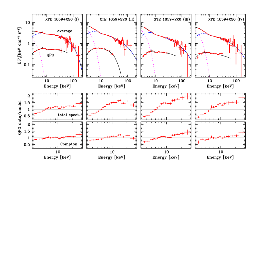
Figure 1: A comparison of the QPO and mean energy spectra in the soft spectral state of XTE J1859+226. Upper panels: time averaged and QPO energy spectra, unfolded using models described in Sec. 2 and Sec. 4.3, respectively. Solid curves show the total spectra, the dotted curve (magenta online) is the disc blackbody component, while the dot-dashed curve (blue online) is the Comptonized component. Lower panels show ratios of the QPO data to various model components: the total time averaged continuum (but without the reprocessed component), and to the time averaged Comptonization continuum only (i.e. the disc and reprocessed components removed). The QPO spectra are harder than the time averaged spectra in this soft state, and they are closer to pure Comptonization continua than to the total continua (i.e. the disc component does not seem to contribute to QPO). The reprocessed component is present in two QPO spectra (I and III; see Table 4).

3.1 Light curves and power density spectra

We used binned and event mode PCA data for the high time resolution spectral analysis. PCA configurations used for each dataset are given in Table 3. We generated light curves in each energy channel using standard tools from the ftools package. We used the binned mode data in the range 3–13 keV and the event mode data above 13 keV. We computed the power density spectra in the Leahy normalization with the white noise subtracted in powspec. Then, we corrected each PDS for background and renormalized to the Miyamoto normalization (i.e., (r.m.s./mean)²), by multiplying by $\frac{S+B}{S^{2}}$, where $S$ and $B$ are source and background count rates, respectively (Berger & van der Klis 1994).

3.2 QPO r.m.s. spectra

We modeled the PDS either as a broken power law continuum with a Lorentz QPO profile, or as a sum of Lorentz profiles describing both the continuum and the QPO (e.g. Nowak 2000). These are phenomenological descriptions, however, since a Lorentz function is a Fourier transform of a damped harmonic oscillator, it can be assumed (in particular in the latter case) that each Lorentzian in the PDS is a signature of a quasi-periodic process with a different degree of coherence. The QPO energy spectrum was then obtained by integrating the QPO Lorentzians over $f$ for different energies.

We constructed response matrices for binned and event mode data using pcarsp (the background correction was performed at the stage of constructing PDS) and we fit the ff-spectra in xspec in order to quantify the spectral trends. We used data in a relatively wide energy range, $\sim 3$–40 keV, but since the PCA data become background dominated above 20–30 keV, any residua and features at 20–40 keV should be treated and interpreted with caution.

4 Results

Here we compare the energy dependent QPO r.m.s. spectra to the time averaged spectra. The latter were described in earlier sections on individual objects. The results are presented in the form of ratios of QPO data to the model components of the time averaged spectra, when the model normalization was adjusted to give smallest possible $\chi^{2}$. These will be useful when we discuss the data in the context of theoretical models in the next Section. We will also perform formal model fits to some of the QPO spectra in order to more quantitatively determine their shape relative to the time averaged spectra.

Our sample contain 14 observations of four objects. Of these 11 observations were performed in soft spectral states while 3 in the hard state.

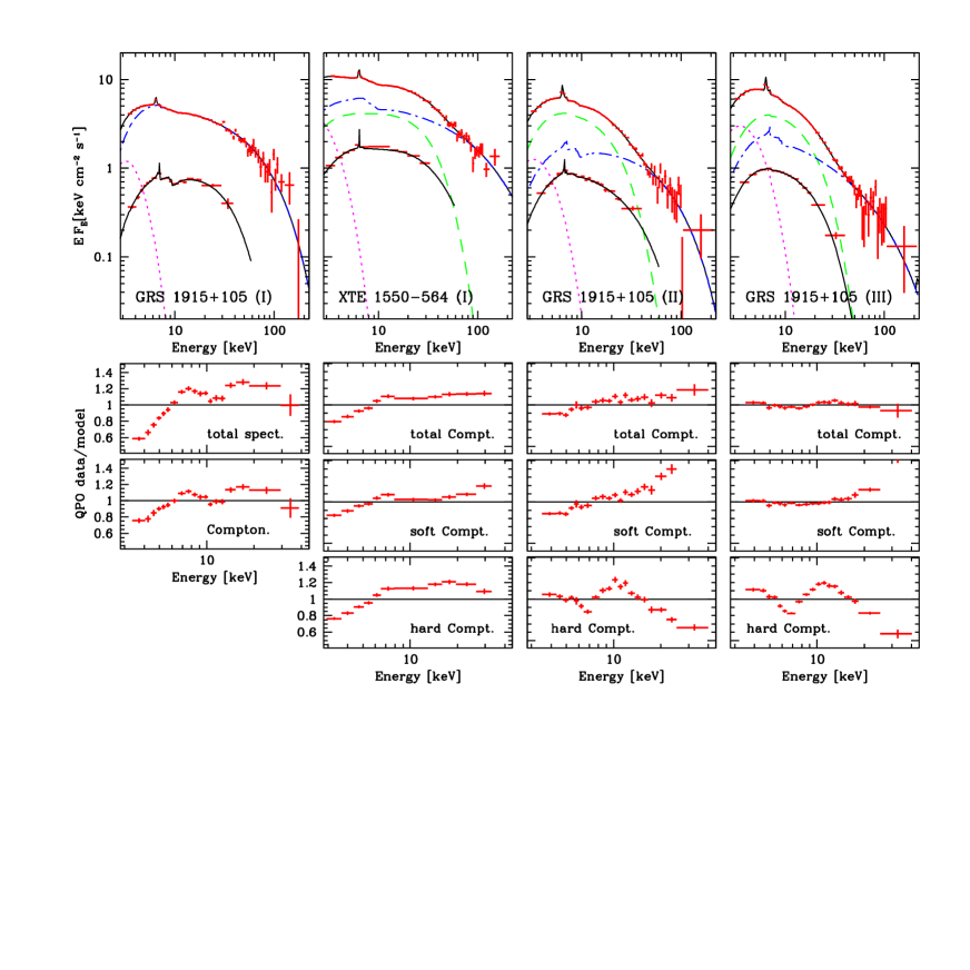
Figure 2: A comparison of the QPO and mean energy spectra in the soft spectral states of GRS 1915+105 and XTE J1550-564. Panels are described in details in Fig. 1. The dashed (green online) curve is the soft Comptonization component. Ratios of the QPO data to: total continuum spectrum, total (two-component) Comptonization, the soft Comptonization and the hard Comptonization, are plotted as labelled.

4.1 Soft state spectra

In the soft state of XTE J1859+226 (Fig 1) the QPO spectra are more similar to the Comptonized component than to the total spectra. This means that the disc blackbody component is not present in the QPO spectra, i.e. it does not participate in the oscillations. The QPO spectra are harder than the Comptonized component in the corresponding time averaged spectrum. Ratios for dataset (III) clearly indicate the presence of the reprocessed component in the QPO spectrum, which will be discussed in more details below.

Similarly, no disc blackbody component in the QPO spectra is observed for GRS 1915+105 (Fig. 2). In all three spectra the QPO data show larger deviations from the total model than from the (total) Comptonized component. In datasets (II) and (III), where the time averaged spectrum requires two Comptonized components, the QPO are most similar to the sum of the two Comptonizations, rather than to either single one of them. In particular, the QPO spectra seem to be much harder than the soft Comptonization.

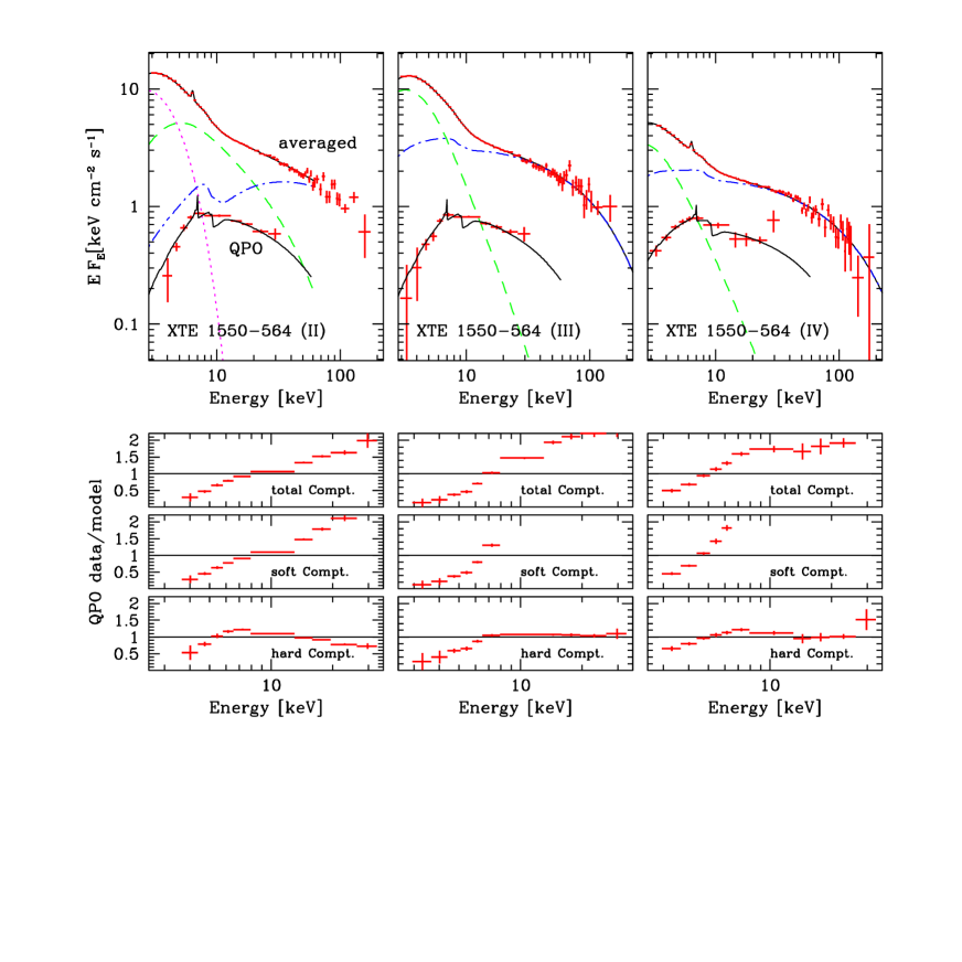
Figure 3: A comparison of the QPO and mean energy spectra in the “anomalous” very high state of XTE J1550-564. Panels are described in details in Fig. 1. Ratios of the QPO data to: total Comptonized continuum, soft Comptonized component and hard Comptonized component are plotted as labelled.

We attempt to fit the QPO data with a modified time averaged Comptonization continuum. We first tie all the parameters of the QPO model, except for normalization, to the parameters of the time averaged spectrum. Fitting the GRS 1915+105 (I) dataset we also set the disc blackbody normalization to 0, so the only free parameter is the normalization of the Comptonized component. The fit is very bad, $\chi^{2}_{\nu}=267/18$ dof. It improves dramatically, when seed photon temperature, $T_{0}$, is free to adjust, $\chi^{2}_{\nu}=42.3/17$ dof. The fit improves further if the continuum slope is left free, $\chi^{2}_{\nu}=35.8/16$. The resulting model has higher $T_{0}\approx 0.95$ keV compared to the $\approx 0.65$ keV in the mean spectrum, and it is harder than the latter, $\Gamma\approx 2.18$ compared to $\approx 2.25$. The fit can be further improved if the reflection amplitude is free to adjust, which will be discussed below.

For GRS 1915+105 datasets (II) and (III) there is a number of ways the time averaged Comptonized components can be modified to fit the QPO spectrum, since there are two Comptonized components in each spectrum (in addition to the disc blackbody). Letting $T_{0}$ (common to the two components) to be free does provide a good fit, with the best fit value again higher than that in the mean spectrum. When the seed photon temperature is fixed, $T_{\rm 0,\ QPO}=T_{\rm 0,mean}$, obtaining a fit of similarly good quality requires freeing at least three parameters: the two spectral slopes and electron temperature of the soft Comptonization.

In the “anomalous” VHS of XTE J1550-564 the QPO spectra are again harder than the time averaged spectra (Fig. 3). The disc blackbody component, even if present in the mean spectrum, is not present in the QPO spectra. The QPO spectra slope above $\approx 7$ keV is similar to that of the hard Comptonization slope in time averaged spectrum, but there is a strong cutoff in QPO spectra below that energy, which formally can be described as a high value of $T_{0}$. We therefore test a model, where the QPO spectrum is equal to the hard Comptonization component in the mean spectrum, but their common seed photon temperature is untied from the disc blackbody temperature or soft Comptonization seed photon temperature, $T_{\rm 0,QPO}=T_{\rm 0,hard}\neq T_{\rm 0,soft}=T_{\rm bb}$. Such a model gives somewhat worse fits to the combined datasets than best models to time averaged data alone. Pairs of $\chi^{2}_{\nu}$ values for the mean spectrum fit (from Section 2) and for the combined mean spectrum and the QPO spectrum fits, are as follows: ($65.8/69=0.95$, $90.8/77=1.18$), ($51.3/71=0.71$, $65.6/81=0.81$) and ($74.5/73=1.02$, $85.1/82=1.04$), for dataset (II), (III) and (IV), respectively. For datasets (III) and (IV) the increase of $\chi^{2}$ is 14.3 and 10.6 per 10 and 9 new dof, respectively. Thus including the QPO data does not significantly worsens these fits. However, when the QPO fits are examined as data/model ratios, they are approximately the same for all datasets. Its the larger error bars on datasets (III) and (IV) (compared to dataset I) that make the fits acceptable. In particular the data show pronounced low energy cutoffs below $\approx 6$ keV, which is not well modelled by the increased $T_{0}$ if the latter is also to fit the mean spectrum. We thus conclude that the QPO data are unlikely to be described simply by the same shape as the hard Comptonizing continuum. This implies that more complicated models, which include spectral variability, must be employed to explain the QPO in these datasets. We intend to explore such models in more details in a future paper.

4.2 Hard state spectra

In the hard spectral state of XTE J1550-564 (dataset V; Fig. 4), the QPO spectrum is somewhat softer than the total spectrum. When the model for the time averaged spectrum is fitted to the QPO data, the best fit model does contain the disc blackbody component ($T_{\rm bb}\approx 0.89$ keV). When the disc blackbody component is removed and the seed photon temperature, $T_{0}$, is fixed at $T_{\rm bb}$, the fit is worse by $\Delta\chi^{2}=7.2$ for one more dof ($\chi^{2}_{\nu}=13.1/10$ vs. $5.7/9$). Now, if $T_{0}$ is free to adjust the fit improves to $\chi^{2}_{\nu}=5.7/9$, but the new $T_{0}=0.54_{-0.54}^{+0.23}$ is lower than $T_{\rm bb}$. Thus, contrary to the QPO spectra in soft states, here the QPO spectrum either contains the disc blackbody component, or the seed photon temperature in QPO spectra is lower than that in time averaged spectra. In either case the QPO spectrum slope is softer than the time averaged spectrum.

In the other two hard state observations, of 4U 1630-47, the QPO slope seems to be similar to the Comptonization slope in the time averaged spectrum, but the residuals suggest somewhat higher $T_{0}$ (Fig. 4). When the time averaged model is renormalized ($\Gamma$ and $T_{0}$ fixed) to the QPO data, the fits have $\chi^{2}_{\nu}=27.5/19$ and $\chi^{2}_{\nu}=25.4/19$ for datasets (I) and (II), respectively. Allowing $\Gamma$ and $T_{0}$ to adjust we obtain best fits with $\chi^{2}_{\nu}=11.0/17$ and $\chi^{2}_{\nu}=17.5/17$, and the confidence contours are plotted in Fig. 5. The contours suggest that the QPO spectra are again somewhat softer and indeed have higher $T_{0}$ than the time averaged spectra, however the difference between the spectral slopes in not highly significant. We note then that for 4U 1630-47 the QPO spectra are closer to the time averged spectra than those of XTE J1550-564 (V). Since the time averaged spectra 4U 1630-47 are softer than the spectra of XTE J1550-564 (V), we might be observing here a transition from the hard state behaviour (as in XTE J1550-564) to the soft state behaviour, where the QPO spectra are harder than the time averaged spectra.

4.3 The reprocessed component in the QPO spectra

We have checked if the reprocessed component is present in the QPO spectra. Firstly, we assume the time averaged continuum as a model for the QPO, and let the reflection parameters, $R$, $\xi$ and $R_{\rm in}$ to be free. Such models do not provide good fits, with only two cases when $\chi^{2}_{\nu}<1.5$ (Table 4; columns a and b). Therefore, although the reprocessed component is present in the model, it is difficult to assess its statistical significance. In the two cases where the fits are acceptable (XTE J1859+226, datasets I and IV), the reflection is significant.

Secondly, we fit the QPO data with the thComp model allowing all its parameters, $\Gamma$, $kT_{\rm e}$ and $T_{0}$ to adjust. The continuum is thus described correctly, which allows for meaningful determination of the presence and parameters of the reprocessed component. We then add the reprocessed component, assuming first a cold matter ($\xi=0$), and then allowing $\xi$ to adjust as well. In Table 4 we present the quality of the initial model (i.e. no reflection) fits, and the $\Delta\chi^{2}$ values when the reprocessed components are added.

Adding the reprocessed component improves the fits in most of the datasets, with ionized reprocessing giving better fits than cold reprocessing. Reduction of $\chi^{2}$ values by 10–60 means that the reprocessed component is highly significant.

Reflection amplitudes in the QPO spectra are generally rather poorly constrained. In the three anomalous very high state spectra of XTE J1550-564 the best fits are obtained for a pure reflected component. However, the ionization parameter in the pure reflection models is rather high, $\xi\sim 10^{5}$, which means that the Fe reprocessing features are not very prominent. The 90 per cent lower limits to $R$ are rather low, nevertheless, reduction of $\chi^{2}$ by 11-22 means that the component is highly significant in at least two of those spectra.

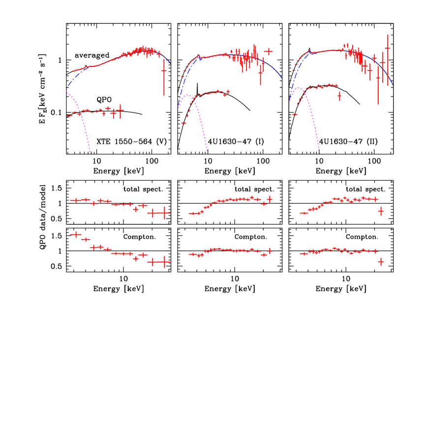
Figure 4: A comparison of the QPO and mean energy spectra in the hard spectral states. Panels are described in details in Fig. 1. Ratios of the QPO data to: total continuum spectrum and the Comptonized continuum are plotted as labelled.

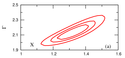
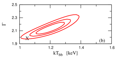
Figure 5: Confidence contours ($\Delta\chi^{2}=2.3,\ 4.6\ {\rm and}\ 9.6$) in the $\Gamma$–$T_{0}$ plane for the QPO spectra from the observations of 4U 1630-47 in the hard state. ’X’ mark the best-fit parameters to the time averaged spectra. The QPO spectra are somewhat softer and have higher $T_{0}$ than the time averaged spectra

5 Discussion

We have applied techniques of Fourier spectroscopy to the analysis of X-ray spectra of a number of black hole X-ray binaries showing QPO in their PDS and we have analysed the QPO r.m.s. spectra. We find that in general the quasi-periodically variable part of X-ray spectra are consistent with thermal Comptonization and they do not require the disc thermal component for their description. This extends previous studies of Churazov et al. (2001) (for soft state of Cyg X-1), and it argues for the origin of the amplitude of the variability (including the QPO) in the hot plasma rather than in the cold disc.

Table 4: Test for the presence of the reprocessed component in the QPO spectra

Object	$\chi^{2,a}/{\rm dof}$	$R^{b}$	$\chi^{2,c}/{\rm dof}$	$\Delta\chi^{2,d}$	$R^{e}$	$\Delta\chi^{2,f}$	$R^{g}$
XTE J1859+226 (I)	18.7/16	$0.47\pm 0.17$	27.0/16	-3.7	0.3	-18.2	$>0.8^{f}$
XTE J1859+226 (II)	76.5/16	0.72	12.4/14	0.0	$0^{+0.3}$	0.0	$0^{+0.4}$
XTE J1859+226 (III)	24.9/14	2.2	16.5/15	-2.7	0.50	-11.0	$>0.2$
XTE J1859+226 (IV)	17.0/15	$0.90^{+0.35}_{-0.30}$	9.86/15	-0.85	0.42	-0.9	$0.2^{+3.5}_{-0.2}$
XTE J1550-564 (I)	17.5/7	1.7	7.2/7	-5.2	$0.62^{+0.63}_{-0.47}$	–	–
XTE J1550-564 (II)	65.1/6	0.6	30.8/7	-15.3	2.1	-22.1	$>0.21^{h}$
XTE J1550-564 (III)	84.6/8	1.3	15.7/8	-4.9	1.3	-11.7	$>0.16^{h}$
XTE J1550-564 (IV)	18.0/6	3.0	10.9/8	-2.5	1.2	-4.8	$>0.08^{h}$
XTE J1550-564 (V)	24.2/9	0.02	5.7/9	–	–	–	–
4U 1630-47 (I)	25.7/17	0.18	15.4/17	-5.4	$0.77^{+0.73}_{-0.58}$	–	–
4U 1630-47 (II)	19.5/16	$0.23^{+0.21}_{-0.13}$	21.4/17	-1.9	0.40	-6.1	$1.00^{+2.5}_{-0.95}$
GRS 1915+105 (I)	45.4/15	1.8	76.4/16	-30.	1.7	-65.9	$>0.8$
GRS 1915+105 (II)	31.0/16	1.7	27.9/16	-7.6	0.97	-10.8	$0.21^{+0.46}_{-0.12}$
GRS 1915+105 (III)	–	–	7.9/15	–	–	–	–

^a $\chi^{2}$/dof from fits of the time averaged spectrum model to the QPO spectra, allowing only the parameters of the reprocessed component and overall normalization to be free
^b Best fit value of $R$ from fits ^a
c $\chi^{2}$/dof from fits of the thComp model to the QPO spectra (all parameters adjustable), without the reprocessed component
^d $\Delta\chi^{2}$ when cold ($\xi=0$) reprocessed component is added, with no relativistic smearing (i.e., one additional parameter)
^e Best fit value of reflection amplitude (or 95 per cent upper limit, $\Delta\chi^{2}=2.71$, when $\Delta\chi^{2}=0$ in column ^d)
^f $\Delta\chi^{2}$ (relative to fits ^c) when ionized reprocessed component is added (2 additional parameters)
^g Best fit value of $R$ from fits ^f
h Best fit obtained for a pure reflected component ($R=+\infty$); 95 per cent lower limit shown
ⁱ the disc blackbody component was included in the QPO model

Comparing the time averaged and the QPO spectra we explicitly find that only one component, a thermal Comptonization (with its Compton reflection) is needed to describe the latter. However, the QPO spectra are in most cases significantly different than the Comptonized component in the time averaged spectra. Qualitatively, we find an interesting anti-correlation: in soft spectral states the QPO spectra are harder than the mean spectra, while they are softer than the mean spectra in hard spectral states. Together with two intermediate cases this forms a continuous sequence. Quantitatively, the differences between the spectra can be described by a difference in spectral indices or seed photons temperatures, or both, with the statistical quality of the various descriptions being approximately the same.

The QPO spectra do contain the reprocessed component. In most datasets their presence is highly statistically significant (99 per cent or better), although the reflection amplitude is rather poorly constrained. Because of that, it is not possible to determine if the amplitude is different than that in the time averaged spectrum.

In Paper I we introduced a phenomenological model of QPO, where the background radial propagation model of broad band variability (Kotov et al. 2001, Życki 2003) is supplemented with quasi-periodic modulation of one or more of the parameters of a Comptonization spectrum. The main parameters include the plasma heating rate, $l_{\rm heat}$, the cooling rate by soft disc photons, $l_{\rm soft}$ (here $l\equiv(L/R)\sigma_{\rm T}/(mc^{3})$ is the compactness parameters), and the amplitude of the reflected component (describing the coupling between the heating and cooling). Our motivation for such a model is that irrespectively of the physical mechanism behind the QPO, the modulation of the emitted X-rays can only be produced by a modulation of one or more of the parameters actually determining the hard X-ray spectrum. We can now discuss our observational results in the light of that model.

QPO spectra harder than the mean spectra can be obtained if the QPO are produced by modulation of the heating rate while the cooling rate does not respond fully to $l_{\rm heat}$ modulation. This produces spectral pivoting around the low energy end of the spectrum, and, in consequence, r.m.s. variability increasing with energy. Such a model might then be applicable to the soft spectral states discussed in this paper. The model predicts a local maximum of the EW of the Fe K$\alpha$ line at the QPO frequency (see fig. 3 in Paper I), but the quality of our data is not sufficient to test this prediction.

QPO spectra softer than the mean spectra can be produced by modulations driven by the cold disc. One possibility here is a modulation of the cooling rate. This results in the spectra pivoting around an energy point intermediate between the low and high energy ends of the spectrum (see also Zdziarski et al. 2002). In the limited energy band, e.g. that of RXTE/PCA, it may correspond to the r.m.s. spectra decreasing with energy.

The cooling rate may be modulated with or without modulation of the seed photons temperature. The difference between the two is that the QPO spectrum is monotonic in energy in the former case but it has a very deep minimum (at the pivot energy) in the latter case (see figs. 4 and 5 in Paper I). Additionally, QPO harmonics appear when $T_{\rm bb}$ is modulated, since the modulation of $l_{\rm soft}$ is then not sinusoidal (even if modulation of $T_{\rm bb}$ is). However, the harmonics are limited to the soft disc component only, unlike in some of our data, for example, XTE J1550-564 (I).

The other possibility of producing a soft QPO spectrum is to modulate the amplitude of the reflected component, $R$, assuming that it also describes the feedback between illuminating hard X-rays and the re-emitted soft disc photons cooling the hot plasma. Because of the coupling, this again generates modulations of $l_{\rm soft}$ and the characteristic spectral pivoting. The most characteristic feature of this model is the strong Fe K$\alpha$ line (and the entire reprocessed component) at $f_{\rm QPO}$, directly resulting from modulations of $R$. Contrary to that, the model with $l_{\rm soft}$ modulation gives either generally weak Fe line, or at least a minimum at $f_{\rm QPO}$. The presence of the reprocessed component (including the Fe K$\alpha$ line) in our QPO spectra makes modulation of $R$ an interesting possibility (see also Miller & Homan 2005).

We note that models from Paper I involving modulation of $l_{\rm soft}$ predict very strong soft component in the QPO spectra, which is not observed. It is rather hard to envision a geometry where the modulated soft flux would enter the hot plasma, but would not be directed towards an observer. Modulation of $R$ also produces some soft component in the QPO spectra, but it appears less prominent than the one from $l_{\rm soft}$ modulation models. Clearly, further development of the models is necessary to fully describe the data.

Another potentially useful diagnostics is the coherence function. While variations in different energy bands are perfectly coherent when $R$ is modulated, the coherence function shows a complex behaviour, with a number of minima, when $l_{\rm soft}$ and/or $T_{\rm bb}$ are modulated. However, distinguishing between the models based on such predicted observables as the EW of the Fe K$\alpha$ line, the coherence function or the hard X-ray time lags would require better data than currently available.

It needs to be emphasized that majority of physical models of QPO envision the QPO as driven by some kind of disc oscillations. However, our interpretation of the energy dependencies of low-$f$ QPO, at least in soft spectral states, would rather point out to modulations of the heating rate in the hot plasma. If so, then those models must find a way of transferring the disc oscillations to the hot plasma with 100 per cent efficiency, i.e. without affecting the disc emission. On the other hand, most of the models were formulated in the context of the high frequency QPO, where the energy dependencies might be different than those for the low-$f$ QPO. The only work where a physical model of the low-$f$ QPO was constructed is that by Giannios & Spruit (2004). They consider oscillations of a hot ion-supported accretion flow coupled to a outer cold disc. The coupling is realized by a number of channels: hard X-rays illuminating the cold disc, hot protons heating the cold disc, the soft disc photons cooling the hot flow. Spectral variability predicted by that model corresponds to our case of modulating the cooling rate, that is, the QPO spectra are softer than the time averaged spectra. This would then be consistent with observed QPO behaviour in the hard state. The overall geometry of a hot inner flow and an outer cold disc fits that state too.

Considering that the usual broad band noise X-ray variability is driven by instabilities and flares in the hot plasma, it is obvious that an important piece of physical understanding is still missing.

6 Conclusions

• The QPO energy spectra are harder than the time average spectra in soft spectral states, but they are softer than the time averaged spectra in the hard state. The QPO spectra are similar in slope to the time averaged spectra, when the latter are intermediate in slope between hard and soft ($\Gamma\approx 2$).

• The disc component is absent in the QPO spectra.

• Comparison of the observational data with simple models of spectral variability suggests that instabilities in the hot plasma drive the low-$f$ QPO in the soft state, while cold disc oscillations drive the QPO in the hard state.

References

- [] Belloni T., van der Klis M., Lewin W. H. G., van Paradijs J., Dotani T., Mitsuda K., Miyamoto S., 1997, A&A, 322, 857
- [] Belloni T., Klein-Wolt M., Méndez M., van der Klis M., van Paradijs J., 2000, A&A, 355, 271
- [] Berger M., van der Klis M., 1994, A&A, 292, 175
- [] Casella P., Belloni T., Homan J., Stella L., 2004, A&A, 426, 587
- [] Churazov E., Gilfanov M., Revnivtsev M., 2001, MNRAS, 321, 759
- [] Cui W., Zhang S. N., Chen W., Morgan E. H., 1999, ApJ, 512, L43
- [] Dieters S. W. et al., 2000, ApJ, 538, 307
- [] Done C., Wardziński G., Gierliński M., 2004, MNRAS, 349, 393
- [] Done C., Życki P. T., Smith D. A., 2002, MNRAS, 331, 453
- [] Giannios D. & Spruit H. C, 2004, A&A, 427, 251
- [] Gierliński M., Zdziarski A. A., 2005, MNRAS, 363, 1349
- [] Gilfanov M., Revnivtsev M., Molkov S., 2003, A&A, 410, 217
- [] Kalemci E., Tomsick J. A., Rothschild R. E., Pottschmidt K., Kaaret P., 2001, ApJ, 563, 239
- [] Kotov O., Churazov E., Gilfanov M., 2001, MNRAS, 327, 799
- [] Kubota A., Done C., 2004, MNRAS, 353, 980
- [] Kubota A., Makishima K., 2004, ApJ, 601, 428
- [] Maccarone T. J., Coppi P. S., 2003, MNRAS, 338,189
- [] Maccarone T. J., Coppi P. S., Poutanen J., 2000, ApJ, 537, L107
- [] Miller J. M., Homan J., 2005, ApJ, 618, L107
- [] Nowak M. A., 2000, MNRAS, 318, 361
- [] Negoro H., Kitamoto S., Mineshige S., 2001, ApJ, 554, 528
- [] Poutanen J., 2001, AdSpR, 28, 267 (astro-ph/0102325)
- [] Poutanen J., Fabian A. C., 1999, MNRAS, 306, L31
- [] Psaltis D., Belloni T., van der Klis M., 1999, ApJ, 520, 262
- [] Psaltis D., 2001, AdSpR, 28, 481 (astro-ph/0012251)
- [] Rao A. R., Naik S., Vadawale S. V., Chakrabarti S. K., 2000, A&A, 360, L25
- [] Remillard R. A., Sobczak G. J., Muno M. P., McClintock J. E., 2002, ApJ, 564, 962
- [] Revnivtsev M., Gilfanov M., 2005, AN, 326, 812
- [] Revnivtsev M., Gilfanov M., Churazov E., 1999, A&A, 347, L23
- [] Revnivtsev M., Gilfanov M., Churazov E., 2001, A&A, 380, 520
- [] Rodriguez J., Corbel S., Tomsick J. A., 2003, ApJ, 595, 1032
- [] Rodriguez J., Corbel S., Hannikainen D. C., Belloni T., Paizis, A., Vilhu O., 2004, ApJ, 615, 416
- [] Rutledge R. E. et al., 1999, ApJS, 124, 265
- [] Sobczak G. J., McClintock J. E., Remillard R. A., Cui W., Levine A. M., Morgan E. H., Orosz J. A., Bailyn C. D. 2000, ApJ, 544, 993
- [] Sobolewska M. A., Życki P. T., 2003, A&A, 400, 553
- [] Tomsick J. A., Kaaret P., 2001, ApJ, 548, 401
- [] Tomsick J. A., Corbel S., Kaaret P., 2001, ApJ, 563, 229
- [] van der Klis M., 2006, in Lewin W. H. G., van der Klis M., eds, Compact Stellar X-ray sources, Cambridge Univ. Press, Cambridge, p. 39 (astro-ph/0410551)
- [] Wijnands R., 2001, Adv. Sp. Res., 28, 469
- [] Wilson C. D., Done C., 2001, MNRAS, 325, 167
- [] Zdziarski A. A., Johnson W. N., Magdziarz P., 1996, MNRAS, 283, 193
- [] Zdziarski A. A., Lubiński P., Smith D. A., 1999, MNRAS, 303, L11
- [] Zdziarski A. A., Poutanen J., Paciesas W. S., Wen L., 2002, ApJ, 578, 357
- [] Życki P. T., 2002, MNRAS, 333, 800
- [] Życki P. T. 2003, MNRAS, 340, 639
- [] Życki P. T., Sobolewska M. A. 2005, MNRAS, 364, 891
- [] Życki P. T., Done C., Smith D. A., 1999, 305, 231