Magnetic Field Confinement in the Corona: The Role of Magnetic Helicity Accumulation

Abstract

A loss of magnetic field confinement is believed to be the cause of coronal mass ejections (CMEs), a major form of solar activity in the corona. The mechanisms for magnetic energy storage are crucial in understanding how a field may possess enough free energy to overcome the Aly limit and open up. Previously, we have pointed out that the accumulation of magnetic helicity in the corona plays a significant role in storing magnetic energy. In this paper, we investigate another hydromagnetic consequence of magnetic-helicity accumulation. We propose a conjecture that there is an upper bound on the total magnetic helicity that a force-free field can contain. This is directly related to the hydromagnetic property that force-free fields in unbounded space have to be self-confining. Although a mathematical proof of this conjecture for any field configuration is formidable, its plausibility can be demonstrated with the properties of several families of power-law, axisymmetric force-free fields. We put forth mathematical evidence, as well as numerical, indicating that an upper bound on the magnetic helicity may exist for such fields. Thus, the accumulation of magnetic helicity in excess of this upper bound would initiate a non-equilibrium situation, resulting in a CME expulsion as a natural product of coronal evolution.

1 Introduction

Coronal mass ejections (CMEs) are a major form of solar activity in the corona. A CME takes $10^{15-16}$ g of plasma from the low corona into the solar wind to disturb the near-Earth space if the CME propagation is directed toward us. Unlike other solar activities such as flares and filament eruptions, CMEs were only first observed when white light coronagraphs were put into space in the 1970s (MacQueen et al. 1974, Howard 1976). Since then, this astrophysical process has caught much attention in the space physics community because of the adverse consequences of CMEs for orbiting satellites.

CMEs are identified as large-scale bright features in white light that move outward through the corona at speeds from 10 to over 2000 km/s (Hundhausen 1999). These are impressive dynamical phenomena that we happen to be able to observe with a certain degree of completeness in both white light (Dere et al. 1999, St. Cyr et al. 2000, Burkepile et al. 2004) as well as in X-ray and EUV bands (Webb & Hundhausen 1987, Hudson & Cliver 2001). In a low-$\beta$ plasma system on the large scales of the corona, we generally believe that MHD processes control the dynamical evolution of the magnetic field and the coronal plasma. In considering CMEs as a MHD phenomena, previous studies have mainly focused on two physical issues: magnetic energy storage and CME initiation.

The energy storage problem is concerned with how much free magnetic energy can be stored in the corona in order for the field to spontaneously open up to infinity during a CME eruption. This issue was first brought up in Aly (1984), and later on in Aly (1991) and Sturrock (1991), where Aly conjectured that a fully-anchored force-free field may not be able to store enough free magnetic energy to drive a CME kinematically, in addition to opening up the field under conditions of high electrical conductivity. This conjecture states that an anchored force-free field cannot store more energy than that of any fully-open field sharing the same boundary flux distribution at the base of the atmosphere, where those fully-open fields have energies bounded from below by a minimum usually referred to as the Aly limit. Many studies have pointed out that the constraint of the Aly Conjecture can be bypassed by relieving one of the conditions assumed in the Conjecture. For example, by relieving the force-free condition an equilibrium field with plasma weight can easily store enough free magnetic energy to drive the CME (Low & Smith 1993, Wolfson & Dlamini 1997, Fong et al. 2002, Low et al. 2003, Zhang & Low 2004, Flyer et al. 2005). Even under the force-free condition, recent studies have showed that the Aly limit can be exceeded if the field contains a detached magnetic flux rope in the corona (Hu et al. 2003, Wolfson 2003, Flyer et al. 2004). The Aly Conjecture can also be bypassed through the topology of multipolar fields. For multipolar fields, a CME-like expulsion only needs to open up one but not all the bipolar fields (Antiochos et al. 1999). In such a situation, the Aly limit associated with opening up the entire field is not the relevant energy threshold; see Zhang & Low (2001) for illustrative examples.

The CME initiation problem is concerned with the sporadic behavior and locations of CME occurrences. CMEs are occurring at an average rate of one to three events per day, with the frequency of occurrence increasing as solar activity intensifies. The catastrophe model (Forbes & Isenberg 1991, Isenberg, Forbes & Demoulin 1993) interprets the CME initiation as a catastrophic loss of equilibrium in a series of quasi-static evolution of magnetic equilibria corresponding to mathematical variations of some model parameters. The flux-emergence trigger model (Chen & Shibata 2000) proposes that the newly-emerged flux near a preexisting flux rope is the trigger of the expulsion.

It might be useful to point out that when we address the magnetic energy storage problem or the CME initiation problem, our underlying thinking tends to take these as two independent issues. However, as we have pointed out in a recent review (Zhang & Low 2005) these two issues can be related by the accumulation of magnetic helicity in the corona as a fundamental MHD process. The accumulation of magnetic helicity in the corona leads to a magnetic energy build-up as a natural product of coronal evolution. Eruptions, as a loss of field confinement, occur when the stored magnetic energy exceeds the Aly limit. In this paper, we take another approach to address the role of magnetic helicity accumulation in the corona. We propose a hydromagnetic conjecture that there is an upper bound on the total magnetic helicity that a force-free field can contain, owing to the fact that a force-free field in an open atmosphere has to self-confine. This conjecture poses a fundamental but mathematically challenging problem in magnetohydrodynamics. We focus our attention in this paper on demonstrating the physical plausibility of the conjecture by using several families of numerical solutions of nonlinear force-free fields to make our physical points.

The paper is organized as follows: In §2, the physical considerations on the roles of magnetic helicity accumulation are addressed, with a particular focus on their connections to the magnetic energy storage and CME initiation. In §3, power-law axisymmetric force-free fields are used to indicate the possible existence of an upper bound on the total magnetic helicity, using both analytical inequalities and numerical solutions. Conclusions and discussions are presented in §4.

2 The Physical Picture and the Conjecture

2.1 Magnetic helicity and its approximate conservation in the corona

Magnetic helicity is defined as $H(V)=\int_{V}{\bf\omega}\cdot{\bf B}dV$, where ${\bf\omega}$ is the vector potential of the vector magnetic field ${\bf B}$ in a volume $V$. It is a physical quantity that quantitatively measures the topological complexity of a magnetic field, such as the degree of linkage and/or twistedness in the field, provided $V$ wholly contains ${\bf B}$. We henceforth refer to $V$ as a a magnetic volume. With this physical quantity, the frozen-in condition in a perfectly conducting plasma can then be stated in terms of the absolute conservation of magnetic helicity in all magnetic sub-volumes as well as of the total magnetic helicity for the whole magnetic volume (Moffatt 1985, see Zhang & Low 2005 for more descriptions).

In a situation of a domain $V$ whose magnetic field ${\bf B}$ threads across its boundary, i.e., the normal magnetic field $B_{n}$ does not vanish across the domain boundary $\partial V$, $H(V)$ is then gauge dependent and is therefore not physical. Magnetic twist and linkage in $V$ then must be described by the relative magnetic helicity denoted by $H_{R}(V)$ introduced by Berger & Field (1984). We will define $H_{R}(V)$ later with the development of the paper. In this paper, we take magnetic helicity to mean either $H(V)$ or $H_{R}(V)$, depending on whichever applies to the given situation.

The frozen-in condition, or the absolute conservation of magnetic helicity in magnetic volumes, must break down in a realistic plasma where the electrical conductivity is very high but not infinite. Electric current sheets can form, and magnetic reconnection will subsequently set in, to dissipate the thin current sheets and change field topology (Parker 1994). However, by a general scaling analysis of resistive processes, Berger (1984) pointed out that the dissipation rate of the total relative magnetic helicity in the corona is orders of magnitude smaller than the release rate of magnetic energy. So the total magnetic helicity in the corona is still approximately conserved despite the occurrences of magnetic reconnection.

The conservation of total magnetic helicity in the corona has a profound influence on the coronal dynamics. Magnetic helicity is continuously being transported into the corona (Kurokawa 1987, Lites et al. 1995, Leka et al. 1996, Zhang 2001, Pevtsov, Maleev & Longcope 2003) with a preferred sign for the two solar hemispheres, positive and negative in the southern and northern hemisphere, respectively (Rust 1994, Pevtsov, Canfield & Metcalf 1995, Bao & Zhang 1998). Moreover, the same opposite signs of helicity are statistically preferred in the two respective hemispheres, negative and positive, respectively, in the northern and southern hemispheres, independent of the solar cycle. Thus, under the approximate conservation of total magnetic helicity, the hemispherical preferred signs of helicity implies an accumulation of magnetic helicity in the two hemispheres. It is this accumulated helicity that, we propose, characterizes the build up of magnetic-energy and when accumulated to a point a magnetic field must open up as an eruption.

2.2 Helicity-energy relationship for fields in finite domains

For a force-free field confined in a finite domain with rigid walls, its total magnetic energy can exceed any value by endowing the field with a sufficiently twisted topology. This can be easily seen from the Virial Theorem of Chandrasekhar (1961), which states that for a force-free field confined in a sphere of radius $r=1$, its total magnetic energy, given in spherical coordinates, is

$$E_{0}=\int_{r<1}{B^{2}\over 8\pi}dV=\frac{1}{4}\int_{r=1}\left(B_{\theta}^{2}+B_{\varphi}^{2}-B_{r}^{2}\right)\sin\theta d\theta~{}~{}.$$ (1)

For a fixed boundary flux $B_{r}$ at $r=1$, the more highly twisted the force-free field is, the greater are the boundary values of the tangential components $B_{\theta}$ and $B_{\varphi}$ at $r=1$, leading to a higher total magnetic energy of the field. Note that force-free solutions can exist in such a domain even if $B_{r}=0$ on $r=1$.

More importantly, if the field is given a total non-zero magnetic helicity $H_{0}$, Woltjer (1958) Theorem sets a ground-level energy above that of the potential field. The Woltjer Theorem produces many constant $\alpha$ force-free fields, each being a local minimum-energy state compared to neighboring fields with the same total magnetic helicity $H_{0}$. The absolutely lowest minimum-energy state, taken from among all those constant $\alpha$ force-free fields, is called the Woltjer state, characterized by a specific constant $\alpha_{0}$. This constant $\alpha_{0}$ of the Woltjer state, together with the given total magnetic helicity $H_{0}$, puts a bound from below for the magnetic energy of the field in a finite domain. That is, the magnetic energy of any field ${\bf B}$ possessing the same total magnetic helicity of $H_{0}$ satisfies the bound:

$$E>|~{}\alpha_{0}H_{0}~{}|~{}~{}.$$ (2)

Applying this theorem to a coronal magnetic field underlying a locally confined coronal structure (Zhang & Low 2003), we can see that the coronal field cannot relax to a potential state as long as the total magnetic helicity is not zero. Magnetic reconnection may set in to release the excess magnetic energy that the coronal field may happen to have, but the field cannot relax to a state that possesses less magnetic energy than that of the Woltjer state. With more and more magnetic helicity brought with a preferred sign into the corona, this ground-level magnetic energy increases with the increasingly accumulated helicity. This is the principal consideration described in Zhang & Low (2005) of the role of the accumulated magnetic helicity in storing magnetic energy for CMEs.

2.3 Confinement issue for fields in unbounded domain

For a force-free field filling an unbounded atmosphere, it has an energy property that is distinct from the one confined in a finite domain with rigid walls. Now, the Virial Theorem of Chandrasekhar (1961) takes a different form and sets a special condition for those fields in force-free equilibrium. For a force-free field outside a sphere of radius $r=1$ in spherical coordinates, its total magnetic energy now takes the form of

$$E_{0}=\int_{r>1}{B^{2}\over 8\pi}dV=\frac{1}{4}\int_{r=1}\left(B_{r}^{2}-B_{\theta}^{2}-B_{\varphi}^{2}\right)\sin\theta d\theta~{}~{},$$ (3)

where we assume that $|{\bf B}|$ spatially decline to zero at $r\rightarrow\infty$ so that the total magnetic energy $E_{0}$ is finite. Here and elsewhere we assume this is the case whenever we treat integration over unbounded domain without explicitly stating this qualification. Since $E_{0}$ should always be positive, the above equation says that no force-free state is possible in $r>1$ domain unless $B_{r}\neq 0$ on $r=1$. With $B_{r}\neq 0$, equation (3) sets an absolute upper bound on the total magnetic energy,

$$E_{max}=\frac{1}{4}\int_{r=1}B_{r}^{2}\sin\theta d\theta~{},$$ (4)

which is uniquely determined by the flux distribution on $r=1$, independent of the twist of the field.

The essence of this hydromagnetic result is that there is an upper bound on the total magnetic energy that a force-free field can attain and this upper bound is determined by its boundary flux at $r=1$. This is equivalent to saying that a force-free field in an unbounded atmosphere requires certain means of confinement to remain in equilibrium. The field with with an arbitrarily large, prescribed degree of twist may not be able to find a force-free state to meet the bound on its total magnetic energy. This is indicated by the the following analysis.

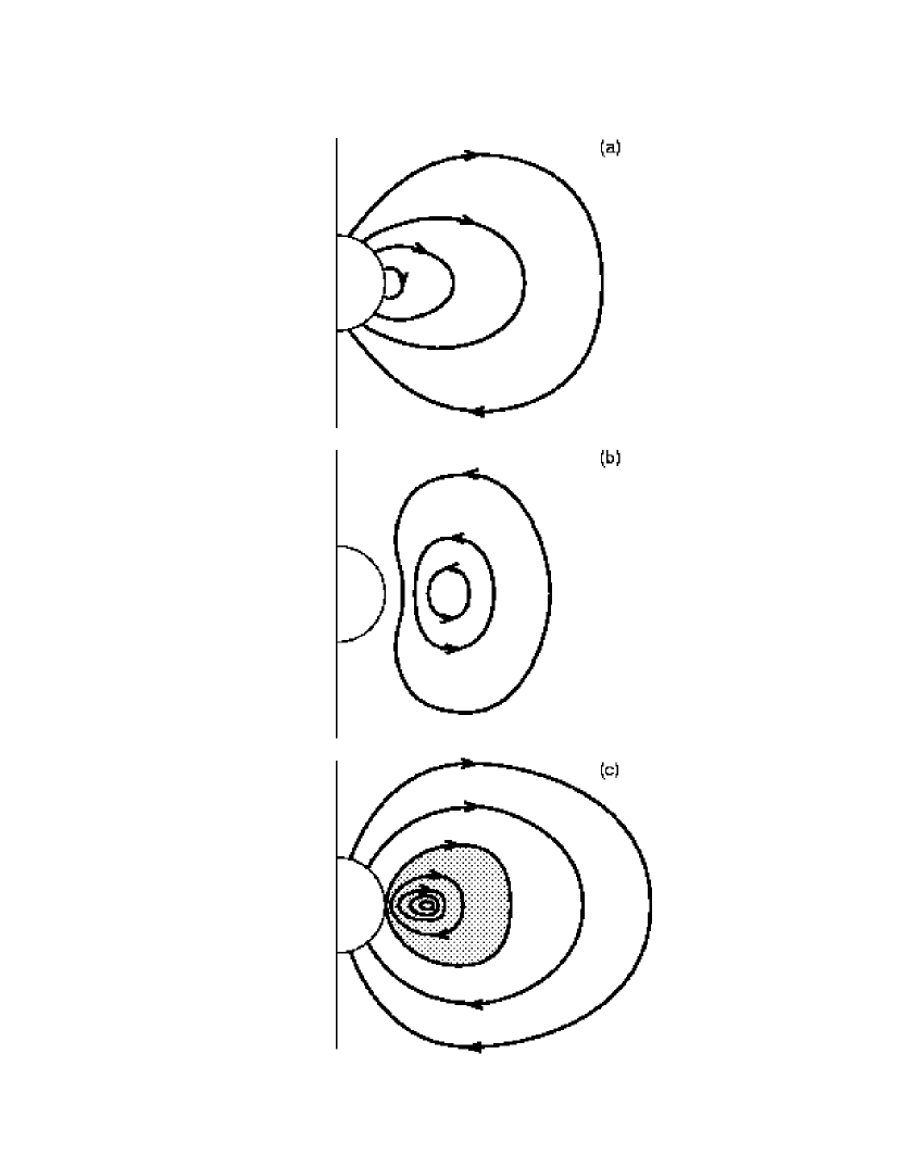
Figure 1: Shown is an axisymmetric magnetic field with its lines of force seen projected on a $r-\theta$ plane, taken from Low (2001). The field lines are directed out of the shown plane if $B_{\varphi}\neq 0$. The middle panel shows an azimuthal field with $B_{r}=0$ on $r=1$, which cannot find an equilibrium. The upper panel shows a potential field with $B_{r}\neq 0$ on $r=1$, meeting the necessary condition for an equilibrium. The bottom panel shows a field also meeting the necessary condition but with a detached flux rope, represented by the closed loops of poloidal projected lines. This configuration can be regarded as a sum of the above two configurations, of a field containing a certain amount of magnetic helicity and finding an equilibrium.

A field completely detached from $r=1$, as drawn in Figure 1b where $B_{r}\equiv 0$, can never be in equilibrium in the absence of other body forces. The only way to hold a flux rope, and hence attain a certain amount of magnetic helicity in the low corona, is to add a $B_{r}\neq 0$ field as in Figure 1a to function as an anchoring agent. The resultant configuration will be the one sketched in Figure 1c, a field containing a certain amount of magnetic helicity and yet finding equilibrium in the $r>1$ domain.

Now imagine we fix the $B_{r}$ distribution on $r=1$ in Figure 1c but arbitrarily increase the total azimuthal flux in the flux rope. This parametric change will take the field closer and closer to the configuration in Figure 1b. We intuitively expect that there would be a parameter representing the field topology crossing over where no force-free equilibrium can exist. We suggest that this critical parameter corresponds to a point of maximum accumulation of magnetic helicity in the atmosphere.

This conjecture intuitively comes from the understanding that the total magnetic helicity cannot be destroyed in the corona at observable time scales. So the corona may thus get a chance to accumulate magnetic helicity of a preferred sign to cross over a threshold bounding the allowable total helicity in a force-free field. A rigorous mathematical bound on the total helicity of a force-free field in $r>1$, in full generality, is needed to prove the conjecture, in parallel to equation (3) for the bound on the total energy of a force-free field. This is a difficult task in mathematical physics. As a first step towards such a proof, we use families of power-law axisymmetric force-free fields of Flyer et al. (2004) to investigate the nature of this conjecture. We focus the rest of our paper on such a study in order to provide a basic understanding of the physical issues.

3 Helicity Bounds for Power-law Axisymmetric Force-free Fields

3.1 A Formula of Total Relative Magnetic Helicity of Axisymmetric Fields

We first derive a formula to calculate the total relative magnetic helicity in axisymmetric magnetic fields. This simple formula is limited to axisymmetric fields but is otherwise quite general, independent of whether the axisymmetric field is in equilibrium or not. We therefore derive the formula from first principles.

Under axisymmetry, we can always write the solenoidal magnetic field ${\bf B}$ in $r>1$ in the form of

$${\bf B}={1\over r\sin\theta}\left[{1\over r}{\partial A\over\partial\theta}~{},~{}-{\partial A\over\partial r}~{},~{}Q(A)\right]~{}.$$ (5)

Here, the flux function $A$ defines the poloidal magnetic field and the function $Q$ defines the toroidal field.

Alternatively, we can also use a vector potential $\omega$ to define a solenoidal magnetic field, where the magnetic field ${\bf B}$ can be derived from the vector potential $\omega$ by the following relationship:

$${\bf B}=\nabla\times\omega~{}~{}.$$ (6)

Then for an axisymmetric magnetic field, $\omega$ takes a form of

$${\bf\omega}={1\over r\sin\theta}\left[{1\over r}{\partial Q^{\prime}\over\partial\theta},-{\partial Q^{\prime}\over\partial r},A^{\prime}\right],$$ (7)

where $Q^{\prime}$ and $A^{\prime}$ are two physical quantities that are related to the functions $A$ and $Q$ by

$$LQ^{\prime}\equiv{\partial^{2}Q^{\prime}\over\partial r^{2}}+{1-\mu^{2}\over r^{2}}{\partial^{2}Q^{\prime}\over\partial\mu^{2}}=-Q~{}~{},$$ (8)

with $\mu=\cos\theta$, and

$$A^{\prime}=A+constant~{}~{}.$$ (9)

These relationships between $Q^{\prime}$, $A^{\prime}$, $Q$ and $A$ can be understood by the following analysis. From the definition of the vector potential and Stokes Theorem, the magnetic flux across any surface $S$ with a boundary $C$ is $F=\int_{S}{\bf B}\cdot d{\bf S}=\int_{C}{\omega}\cdot d{\bf l}$ where $d{\bf l}$ is a path element along $C$. Therefore, the vector potential $\omega$ carries information about the magnetic flux across surfaces. Application of this relation with $\omega$ given by equation (7) for an axisymmetric field shows that the function $Q^{\prime}$ carries information on the azimuthal flux, as implied by the relationship between $Q^{\prime}$ and $Q$ in equation (8), and the function $A^{\prime}$ carries information about the poloidal flux as expressed by equation (9).

The $constant$ in equation (9) can be used to take care of the physical requirement that $A^{\prime}$ should be zero along the polar axes. Without loss of generality, we set this $constant$ to zero, which is equivalent to setting the flux function $A$ to zero along the polar axes.

Suppose we are given the field ${\bf B}$ in the unbounded space $r>1$ denoted as $V$. This field has a flux anchored to the inner boundary $r=1$ so that the classical helicity of Woltjer is not gauge invariant and we must use instead the relative helicity of Berger & Field (1984). This is given by the formula derived in Berger (1985):

$$H_{R}=\int_{V_{a}}\omega^{p}_{a}\cdot{\bf B}^{p}_{a}\hskip 5.69054ptdV+\int_{V}\omega\cdot{\bf B}\hskip 5.69054ptdV~{},$$ (10)

which involves extending the domain $V$ to the spherical region $r<1$ denoted as $V_{a}$ where ${\bf B}_{a}^{p}$ is a potential field with vector potential $\omega_{a}^{p}$. This potential field continues into the given field ${\bf B}$ across the boundary with continuity of $B_{r}$. The important point here is that $H_{R}$ is independent of the gauge and is a physical quantity describing the topological complexity of the field ${\bf B}$ in $r>1$. We calculate $H_{R}$ as follows.

The solenoidal condition requires

$${\bf B}_{a}^{p}\cdot{\bf r}\hskip 5.69054pt|_{r=1}={\bf B}\cdot{\bf r}\hskip 5.69054pt|_{r=1}$$ (11)

for the continuity of the normal field across $r=1$. Equivalently, in terms of the vector potential, we require

$$\omega_{a}^{p}\times{\bf r}\hskip 5.69054pt|_{r=1}=\omega\times{\bf r}\hskip 5.69054pt|_{r=1}~{},$$ (12)

for the continuity of the tangential components of the vector potential (Berger & Field 1984).

Equation (12) requires that both $A$ and ${\partial Q^{\prime}\over\partial r}$ are continuous across $r=1$. The continuity of $A$ across $r=1$ is just equation (11) and the normal flux of ${\bf B}$ at $r=1$ determines a unique potential field ${\bf B}^{p}_{a}$ in $V_{a}$. This potential field is generated by a flux function $A_{a}^{p}$, with $Q=0$. We take $Q^{\prime}=0$ everywhere in $V_{a}$, which is consistent with equation (8) where $Q=0$, as a selected gauge. Hence, we have

$${\bf B}^{p}_{a} = {1\over r\sin\theta}\left({1\over r}{\partial A_{a}^{p}\over\partial\theta}{\hat{r}}-{\partial A_{a}^{p}\over\partial r}{\hat{\theta}}\right)$$

$$\omega^{p}_{a} = {A\over r\sin\theta}{\hat{\varphi}},$$ (13)

which are two orthogonal vectors so that $\int_{V_{a}}\omega_{a}^{p}\cdot{\bf B}_{a}^{p}dV=0$ and $H_{R}$ in equation (10) then contains only the contribution from $r>1$.

Now we have the total relative magnetic helicity in $r>1$ as

$$H_{R}=\int_{r>1}{\bf\omega}\cdot{\bf B}dV=2\pi\int_{r>1}{1\over r^{2}(1-\mu^{2})}\left[\nabla Q^{\prime}\cdot\nabla A+AQ\right]r^{2}drd\mu~{}~{},$$ (14)

where we have the geometric boundary conditions that both $Q^{\prime}$ and $A$ vanish at the polar axes and the gradients of these two functions with distance vanish sufficiently fast at infinity. These conditions and integrations by parts allow us to rewrite

$$\int_{r>1}{1\over r^{2}(1-\mu^{2})}\nabla Q^{\prime}\cdot\nabla Ar^{2}drd\mu=\int_{r>1}drd\mu{AQ\over 1-\mu^{2}}-\int_{-1}^{1}{d\mu\over 1-\mu^{2}}\left[A{\partial Q^{\prime}\over\partial r}\right]_{r=1}~{}.$$ (15)

And then the total relative magnetic helicity is given by:

$$H_{R} = 4\pi\int_{r>1}drd\mu{AQ\over 1-\mu^{2}}-2\pi\int_{-1}^{1}{d\mu\over 1-\mu^{2}}\left[A{\partial Q^{\prime}\over\partial r}\right]_{r=1}$$ (16)

$$= 4\pi\int_{r>1}drd\mu{AQ\over 1-\mu^{2}}~{}~{},$$

a simple form of an integral to calculate the total relative magnetic helicity in $r>1$.

Note this formula can also be rewritten as

$$H_{R}=4\pi\int_{r>1}A\times B_{\varphi}rdrd\theta$$ (17)

and it gives a physical meaning of this simple form of helicity formula: The total relative magnetic helicity in axisymmetric fields is just a simple convolution of the local wrapping of the azimuthal flux element $B_{\varphi}rdrd\theta$ with the poloidal flux $A$.

3.2 Power-law axisymmetric force-free fields

We adopt the families of numerical force-free fields from Flyer et al. (2004) where $Q$ as a strict function of $A$ has the form of

$$Q^{2}(A)=\frac{2\gamma}{n+1}A^{n+1}~{}.$$ (18)

Here $n$ is an odd constant index required to be no less than 5 in order for the field to possess finite magnetic energy in $r>1$ and $\gamma$ is a free parameter which we choose to be positive without loss of generality. We refer this family of force-free fields power-law axisymmetric force-free fields in this paper.

Taking this form of $Q$, the force-free condition, that is,

$$\left(\nabla\times{\bf B}\right)\times{\bf B}=0~{}~{},$$ (19)

reduces to the following governing equation for flux function $A$:

$${\partial^{2}A\over\partial r^{2}}+{1-\mu^{2}\over r^{2}}{\partial^{2}A\over\partial\mu^{2}}+\gamma A^{n}=0~{}~{}.$$ (20)

This governing equation was solved numerically as a boundary value problem within domain $r>1$ in Flyer et al. (2004), subject to the prescribed boundary flux distribution

$$A|_{r=1}=\sin^{2}\theta~{}~{}.$$ (21)

We refer interested readers to that paper for various properties of this family of force-free fields for the cases of $n=5,7,9$.

Note that although $\gamma>0$ is a free parameter, it actually has a least upper bound $\gamma_{0}$ above which no solution of the boundary value problem can exist. As shown in Flyer et al. (2004), with the boundary condition (21), for each fixed $n$,

$$\gamma<\gamma_{0}={\frac{2(n+1)(2n+1)!!}{3(2n)!!}}~{}.$$ (22)

3.3 A bound on the total magnetic helicity for a fixed $n$

The Virial Theorem expresses the total magnetic energy of a force-free magnetic field ${\bf B}$ in $r>1$ in terms of a surface integral given by equation (3). Aly (1988) presented a “generalized scalar virial equation” that expresses the total magnetic energy in other forms. Writing $B_{t}^{2}=B_{\theta}^{2}+B_{\varphi}^{2}$ and introducing an arbitrary function $f(r)$ with derivative $f^{\prime}(r)$, Aly derived

$$\int_{r>1}\left[f(B_{r}^{2}+B_{t}^{2})+rf^{\prime}(B_{t}^{2}-B_{r}^{2})\right]dV~{}~{}=~{}~{}f(r=1)\int_{r=1}(B_{r}^{2}-B_{t}^{2})dS~{}~{}.$$ (23)

For our purpose, we set $f=r$ to obtain

$$\int_{r>1}\left[r(B_{r}^{2}+B_{t}^{2})+r(B_{t}^{2}-B_{r}^{2})\right]dV=\int_{r=1}(B_{r}^{2}-B_{t}^{2})dS~{}~{}.$$ (24)

This leads to an alternative expression of total magnetic energy of force-free fields as

$$E_{0} = \frac{1}{4\pi}\int_{r>1}r\left(B_{\theta}^{2}+B_{\varphi}^{2}\right)dV~{}~{}.$$ (25)

From this form of $E_{0}$, we then have

$$E_{0} \geq \frac{1}{4\pi}\int_{r>1}rB_{\theta}^{2}dV$$ (26)

$$E_{0} \geq \frac{1}{4\pi}\int_{r>1}rB_{\varphi}^{2}dV$$ (27)

and

$$E_{0}^{2} \geq \int_{r>1}\frac{rB_{\theta}^{2}}{4\pi}dV\int_{r>1}\frac{rB_{\varphi}^{2}}{4\pi}dV~{}~{}.$$ (28)

Consider Cauchy-Schwartz inequality

$$\int_{X}f^{2}dx\int_{X}g^{2}dx\geq\left(\int_{X}fgdx\right)^{2}~{}~{},$$ (29)

which relates two functions $f$ and $g$ in space $X$, where $dx$ is the spatial integration element. Applying Cauchy-Schwartz inequality to inequality (28), we get

$$E_{0}^{2} \geq \left(\frac{1}{4\pi}\int_{r>1}rB_{\theta}B_{\varphi}dV\right)^{2}~{}~{}~{}.$$ (30)

The right hand side of this inequality contains an integral of the product of the poloidal field $B_{\theta}$ with the toroidal field $B_{\varphi}$, suggestive of the formula (16) of the relative magnetic helicity.

By equation (16) the total relative magnetic helicity in $r>1$ of a power-law axisymmetric force-free field is

$$H_{R} = 4\pi\sqrt{\frac{2\gamma}{n+1}}\int_{-1}^{1}{d\mu\over 1-\mu^{2}}\int_{1}^{\infty}A^{\frac{n+3}{2}}dr~{}~{}.$$ (31)

Evaluate the right hand side of inequality (30) we obtain

$$\frac{1}{4\pi}\int_{r>1}rB_{\theta}B_{\varphi}dV = -\frac{1}{2}\int_{-1}^{1}{d\mu\over 1-\mu^{2}}\int_{1}^{\infty}rdr{\partial A\over\partial r}\sqrt{\frac{2\gamma}{n+1}}A^{\frac{n+1}{2}}$$ (32)

$$= \frac{1}{2}\int_{-1}^{1}{d\mu\over 1-\mu^{2}}[{2\over n+3}\sqrt{\frac{2\gamma}{n+1}}A^{\frac{n+3}{2}}]_{r=1}$$

$$+\frac{1}{2}\int_{-1}^{1}{d\mu\over 1-\mu^{2}}\int_{1}^{\infty}dr{2\over n+3}\sqrt{\frac{2\gamma}{n+1}}A^{\frac{n+3}{2}}~{}~{},$$

with an integration by part. Using the boundary condition at $r=1$ to evaluate the first term and denoting it as ${2\over n+3}\sqrt{\frac{2\gamma}{n+1}}c_{0}$, then

$$c_{0}=\frac{1}{2}\int_{-1}^{1}{d\mu\over 1-\mu^{2}}[A^{\frac{n+3}{2}}]_{r=1}>0$$ (33)

is a constant independent of $\gamma$. Inequality (30) now takes the form of

$$(\frac{n+3}{2})^{2}E_{0}^{2} \geq \left(\sqrt{\frac{2\gamma}{n+1}}c_{0}+\frac{H_{R}}{8\pi}\right)^{2}~{}~{},$$ (34)

and we have achieved a bound on $H_{R}$.

A simple analysis reduces inequality (34) to the form of

$$-8\pi\left[{n+3\over 2}E_{0}+\sqrt{{2\gamma\over n+1}}c_{0}\right]\leq H_{R}\leq 8\pi\left[{n+3\over 2}E_{0}-\sqrt{{2\gamma\over n+1}}c_{0}\right].$$ (35)

Since $c_{0}$ is defined strictly by the boundary condition, inequality (35) shows that the magnitude of $H_{R}$ is bounded from above by bounds that are fixed for each given $n$.

The above inequality shows that $|H_{R}|$ is bounded for each fixed $n$. However, this does not assure us that a single bound $H_{max}>0$ exists such that $|H_{R}|<H_{max}$ for all $n$, because the upper and lower bounds go to $\pm\infty$ as $n\rightarrow\infty$. A tighter bound on $H_{R}$ is then motivated to be found and will be presented in §3.5.

3.4 Numerical evidence

It is useful for us to use those numerical solutions in Flyer et al. (2004) to examine some helicity properties of this family of power-law axisymmetric force-free fields. In Flyer et al. (2004), Newton’s iteration combined with a pseudo-arc length continuation scheme was used to solve the nonlinear partial differential equation (20) in the unbounded domain $r>1$ for the boundary condition (21). It was found that iterations converge to solutions only for a finite range of $\gamma$ for a fixed index $n$, as indicated by inequality (22). In addition, the solution $A$ was found to be a multi-valued function of $\gamma$, i.e. for a given value of $\gamma$ multiple solutions can exist. These multiple functions can be pieced into a single solution curve as a function of $\gamma$ joined at turning points. The pseudo-arc length continuation scheme was used to march along the solution curve for a given $n$ and to pass through the turning points in the parameter space where the Jacobian of the Newton’s iteration become singular.

Each point on the obtained solution curves describes a power-law axisymmetric force-free field in $r>1$ with a total magnetic energy $E_{0}$, a total azimuthal flux

$$F_{\varphi}=\int_{r>1}B_{\varphi}rdrd\theta~{},$$ (36)

and a total relative magnetic helicity $H_{R}$ given by equation (16). Flyer et al. (2004) characterized their solutions in terms of $E_{0}$ and $F_{\varphi}$, but not $H_{R}$. The approximate conservation law for $H_{R}$ naturally suggests the use of $H_{R}$ to characterize the twisted state of the force-free field in $r>1$. In Figure 2 we display the variation of $E_{0}$ and $F_{\varphi}$ with $\gamma$ for the $n=5,7,9$ solution curves, taken from Flyer et al. (2004), together with the respective variations of $H_{R}$ for these curves.

For each of the $n=5,7,9$ solution curves, Flyer et al. (2004) found that $F_{\varphi}$ is bounded to be of the order of twice the total poloidal flux given by boundary condition (21). This numerical evidence indicates that force-free fields can only self-confine its magnetic pressure by its tension force provided its azimuthal flux is less than a bound determined by its poloidal flux fixed by the boundary condition. These are indicated in Figure 2 by the azimuthal flux $F_{\varphi}$ monotonically increases from 0 to its maximum value along a solution curve, noting in particular that the maximum value of $F_{\varphi}$ is in each case less than 2 and not sensitive to $n$. The corresponding relative helicity $H_{R}$ shows interesting undulations superposed on a general trend of monotonic increase along the solution curves, showing a bound on $H_{R}$ less than 15 and not sensitive to $n$. These numerical solutions provide a basis for the suggestion that the total relative magnetic helicity of the three families of power-law axisymmetric force-free fields is also bounded by a suitably defined bound that depends only on the boundary flux distribution.

Figure 3 presents these solutions again, but are plotted for the total magnetic helicity (left panels) or for the total magnetic helicity divided by the total magnetic energy (right panels) against the azimuthal flux. These plots show that the total magnetic helicity increases nearly monotonically with the increasing azimuthal flux, which confirms our intuition that the confinement issue discussed in terms of the azimuthal flux is not much different from the discussion in terms of magnetic helicity. However, the total magnetic helicity is known to be conserved in the corona and therefore accumulated in the corona, whereas the physics is less specific whether the azimuthal flux is conserved in the corona or not.

Another interesting observation from Figure 3 is that, the ratio between the total magnetic helicity and the total magnetic energy shows a better monotonic variation with the azimuthal flux than does the magnetic helicity itself. This may reflect a general relationship among the three quantities. Notice that inequality (35) suggests that $H_{R}/E_{0}$ is roughly smaller than $4\pi(n+3)$ which is confirmed by the numerical solutions. However, the bound obeyed by the numerical solutions is a lower or tighter upper bound. That is, $H_{R}/E_{0}<9\pi<4\pi(n+3)=(32-48)\pi$, the last term taken from inequality (35). This hints that the upper bound we have found by inequality (35) is not a stringent bound and that lower upper bounds may exist.

3.5 Inequality relating total magnetic helicity to azimuthal flux and magnetic energy

The numerical relationships among $E_{0}$, $F_{\varphi}$ and $H_{R}$ in Figure 3 suggest that a rigorous relationship may exist between these three physical quantities, at least, for the power-law force-free fields. This rigorous relationship is derived in this subsection by first introducing

$$E_{\varphi}=\frac{1}{8\pi}\int_{r>1}B_{\varphi}^{2}dV~{},$$ (37)

which is the contribution of the azimuthal field component to the total magnetic energy.

As an extension of Cauchy-Schwartz inequality, Holder inequality states that, given any two functions $f$ and $g$ in space $X$ with spatial integration element $dx$, we have

$$\left(\int_{X}f^{k}dx\right)^{1/k}\left(\int_{X}g^{k^{\prime}}dx\right)^{1/k^{\prime}}\geq\int_{X}fgdx~{},$$ (38)

where $k>1$ and is related to $k^{\prime}$ by

$$\frac{1}{k}+\frac{1}{k^{\prime}}=1~{}~{}.$$ (39)

The inequality (38) reverses direction if $k<1$ while k still relates to $k^{\prime}$ by equation (39).

Applying Holder inequality with

$$f = A^{2},$$ (40)

$$g = A^{m},$$ (41)

$$k = m+1,$$ (42)

$$k^{\prime} = 1+1/m,$$ (43)

$$dx = {drd\theta\over\sin\theta},$$ (44)

we have

$$\left(\int_{r>1}A^{2m+2}{drd\theta\over\sin\theta}\right)^{\frac{1}{m+1}}\left(\int_{r>1}A^{m+1}{drd\theta\over\sin\theta}\right)^{\frac{m}{m+1}}\geq\int_{r>1}A^{m+2}{drd\theta\over\sin\theta}~{},$$ (45)

where $m=\frac{n-1}{2}$ and is an integer greater than 1. With the power-law definition of $Q$ in equation (18), it is easy to show that

$$E_{\varphi} = \frac{\gamma}{4(m+1)}\int_{r>1}A^{2m+2}{drd\theta\over\sin\theta}~{}~{},$$ (46)

$$F_{\varphi} = \sqrt{\frac{\gamma}{m+1}}\int_{r>1}A^{m+1}{drd\theta\over\sin\theta}~{}~{},$$ (47)

$$H_{R} = 4\pi\sqrt{\frac{\gamma}{m+1}}\int_{r>1}A^{m+2}{drd\theta\over\sin\theta}~{}~{}.$$ (48)

Now inequality (45) leads to

$$H_{R}\leq 4\pi F_{\varphi}^{\frac{m}{m+1}}E_{\varphi}^{\frac{1}{m+1}}\left[\frac{16(m+1)}{\gamma}\right]^{\frac{1}{2m+2}}~{}.$$ (49)

Define

$$y = \frac{H_{R}}{4\pi F_{\varphi}^{\frac{m}{m+1}}E_{\varphi}^{\frac{1}{m+1}}\left[\frac{16(m+1)}{\gamma}\right]^{\frac{1}{2m+2}}}~{}.$$ (50)

Inequality (49) is then equivalent to say that $y\leq 1$.

Figure 4 presents the $y$ values, plotted against $F_{\varphi}$, for the families of $n=5,7,9$ fields, using numerical solutions in Flyer et al. (2004) again. We see that the y values for these three families of fields vary between 0.75 to 0.95, with a tendency for the overall y values to increase with the $n$ values. The fact that these y values are all less than 1 is just the verification of inequality (49), which is rigorous for all power-law axisymmetric force-free fields. The more interesting point is that these y values can get close to 1. This implies that we are getting close to finding a stringent bound on the total magnetic helicity by inequality (49), a more stringent inequality than inequality (35) is.

As pointed out by the referee, an interesting feature from Figure 4 is that our y values do not vanish to zero when both the total magnetic helicity and azimuthal flux vanish. Inserting equations (46)-(48) into equation (50), we find that our y values can be represented as

$$y=\frac{\int_{r>1}A^{m+2}{drd\theta\over\sin\theta}}{(\int_{r>1}A^{m+1}{drd\theta\over\sin\theta})^{\frac{m}{m+1}}(\int_{r>1}A^{2m+2}{drd\theta\over\sin\theta})^{\frac{1}{m+1}}}~{},$$ (51)

which shows that values of y are not directly dependent on $\gamma$. Applying potential field $A=\frac{\sin^{2}\theta}{r}$, we get $y=0.88,0.90,0.92$ for $n=5,7,9$ respectively. These numbers are consistent with the tendencies of y values in Figure 4.

Now multiply across equation (20) with flux function $A$ and then integrate it with the element ${drd\theta\over\sin\theta}$ to get

$$\int_{r>1}(m+2)Q^{2}dr{d\theta\over\sin\theta}=\int\left[A{\partial A\over\partial r}\right]_{r=1}{d\theta\over\sin\theta}+\int_{r>1}\left(B_{r}^{2}+B_{\theta}^{2}+B_{\varphi}^{2}\right)dr{d\theta\over\sin\theta}~{}.$$ (52)

The left-hand side of the equation is proportional to $E_{\varphi}$, whereas, on the right hand side, the first term is bounded by the Chandrasekhar Virial Theorem and the second term is proportional to the magnetic energy $E_{0}$. Direct derivation then gives

$$(m+2)E_{\varphi}\leq\frac{4}{3}E_{max}+E_{0}~{}~{},$$ (53)

where $E_{max}$ is given by equation (4).

As $E_{0}<E_{max}$ and $E_{max}$ is bounded by the boundary condition at $r=1$, the above inequality (53) shows that $(m+1)E_{\varphi}$ is also bounded. In consequence, we have $E_{\varphi}\rightarrow 0$ as the free index $m\rightarrow\infty$. This means that as we go to higher and higher $n$, the energy contributed by $B_{\varphi}^{2}$ becomes negligible. Much of the energy in the sum $B_{\theta}^{2}+B_{\varphi}^{2}$ is in the $\theta$ component. In physical terms, we conclude that for the large-$n$ families of fields, the flux rope in the field is wounded so tightly that it approaches the highly localized structure of a line current or a sheet current outside of which $B_{\varphi}$ is negligible. In other words, the free energy is stored as $B_{\theta}$ in this exterior region associated with the line or sheet current.

Applying inequality (53) to inequality (49), we get

$$H_{R}\leq 4\pi F_{\varphi}^{\frac{m}{m+1}}\left[\frac{16(m+1)(\frac{4}{3}E_{max}+E_{0})}{(m+2)^{2}~{}\gamma}\right]^{\frac{1}{2m+2}}~{},$$ (54)

a tight bound on $H_{R}$.

To study this inequality, let us define

$$C_{1} = \left[\frac{16(m+1)}{(m+2)^{2}}\right]^{\frac{1}{2m+2}}~{},$$ (55)

$$C_{2} = \left[\frac{16(m+1)(\frac{4}{3}E_{max}+E_{0})}{(m+2)^{2}~{}\gamma}\right]^{\frac{1}{2m+2}}=C_{1}\left(\frac{\frac{4}{3}E_{max}+E_{0}}{\gamma}\right)^{\frac{1}{2m+2}}~{}.$$ (56)

Inequality (54) now can be written as

$$H_{R}\leq 4\pi F_{\varphi}^{\frac{m}{m+1}}C_{2}~{}.$$ (57)

The top panel of Figure 5 shows the $C_{2}$ values, plotted against the azimuthal fluxes, for $n=5,7,9$ families of fields. We see that as $n$ increases from $n=5$ to $n=9$, the modulation of $C_{2}$ values decreases, with the $C_{2}$ values approaching $1$. This indicates that as $n\rightarrow\infty$, $C_{2}$ values tend to 1. This can be understood by the following analysis. $C_{2}$ is a multiplication of $C_{1}$ and $\left(\frac{\frac{4}{3}E_{max}+E_{0}}{\gamma}\right)^{\frac{1}{2m+2}}$. Since $E_{max}$, $E_{0}$ and $\gamma$ are all bounded, the term $\left(\frac{\frac{4}{3}E_{max}+E_{0}}{\gamma}\right)^{\frac{1}{2m+2}}$ goes to 1 as $m\rightarrow\infty$ except for $\gamma=0$. When $\gamma=0$, $H_{R}=0$. This is the trivial potential field and is not an interesting field for our consideration of helicity upper bound. Owing to its mathematical form in equation (55), $C_{1}$ approaches 1 as $m\rightarrow\infty$. This is indicated by the plot in the bottom panel of Figure 5, where $C_{1}$ values are plotted against $m$ and are approaching to 1 as $m$ increases. So, on the limit of $n\rightarrow\infty$ or, equivalently, $m\rightarrow\infty$,

$$C_{1} \rightarrow 1~{},$$

$$C_{2} \rightarrow 1~{},$$

$$F_{\varphi}^{\frac{m}{m+1}} \rightarrow F_{\varphi}~{},$$ (58)

and hence we have

$$H_{R}\leq 4\pi F_{\varphi}~{}.$$ (59)

Now we see that in the limit of $n\rightarrow\infty$, the bound on $H_{R}$ reduces to a problem of finding an upper bound on $F_{\varphi}$. The force-free solutions of Flyer et al. (2004) suggest that such an upper bound exists (see also Figure 2 in this paper). Our tighter inequality (59) has thus provided a more stringent bound on $H_{R}$ that had eluded from the lose inequality (35).

Figure 6 shows the variations of $H_{R}/(4\pi F_{\varphi})$ against $\gamma$ for $n=5,7$ and $9$ families. These plots show that the relationship $H_{R}\leq 4\pi F_{\varphi}$ we derived for $n\rightarrow\infty$ is also valid for $n=5,7,9$ families. So this relationship may be a general relationship that is valid for all $n$ values. If this is true, it tells us that the upper bound on the total magnetic helicity is a less stringent upper bound than that on the total azimuthal flux.

4 Conclusions and Discussions

In this paper we proposed a hydromagnetic conjecture that there is an upper bound on the total magnetic helicity that a force-free field in an unbounded domain can contain. Observations have shown that accumulations of helicity with a preferred sign takes places in the two solar hemispheres. If our conjecture is valid, the relentless accumulation of magnetic helicity in the corona will lead to a CME-type eruption as a natural and unavoidable product of coronal evolution. This conjecture deserves further investigation to find a mathematical rigorous proof, or disproof. For the present, evidence for and implications of this conjecture can be found in the several families of power-law axisymmetric force-free fields governed by equation (20).

We derived two rigorous inequalities (S1 and S2 in Table 1) by applying the Cauchy-Schwartz and Holder inequalities, respectively. The former (S1 in Table 1 or Equation (35) in the text) puts an absolute upper bound on the magnitude of total magnetic helicity for each fixed index $n$. This inequality is simple and rigorous but it is not tight for our purpose, with the bounds increasing monotonically with $n$. The second inequality (S2 in Table 1) relates total magnetic helicity, azimuthal flux and magnetic energy together in an interesting way, which presents a more stringent bound than S1 does.

Inequality S2 is further reduced to the simple form of Inequality S3 in Table 1 when $n$ goes to infinity. We have not proved that the simple form of Inequality S3 is valid for all $n$ although the numerical data of Figure 6 suggest it is. The validation of Inequality S3 for large $n$ is sufficient for our purpose, which is to remove our main concern arising from Inequality S1 of whether the total helicity is still bounded when $n$ becomes very large. Inequality S3 together with the numerical results from Flyer et al. (2004) suggest that such an upper bound on the total magnetic helicity exists even when $n$ increases without bound.

Table 1: Significant equation and inequalities derived in the paper

Number	Equation or Inequality	No. in the paper
S0	$H_{R}=4\pi\int_{r>1}A\times B_{\varphi}rdrd\theta$	(Equ. 17)
S1	$-8\pi\left[{n+3\over 2}E_{0}+\sqrt{{2\gamma\over n+1}}c_{0}\right]\leq H_{R}\leq 8\pi\left[{n+3\over 2}E_{0}-\sqrt{{2\gamma\over n+1}}c_{0}\right]$	(Equ. 35)
S2	$H_{R}\leq 4\pi F_{\varphi}^{\frac{m}{m+1}}\left[\frac{16(m+1)(\frac{4}{3}E_{max}+E_{0})}{(m+2)^{2}~{}\gamma}\right]^{\frac{1}{2m+2}}$	(Equ. 54)
S3	$H_{R}\leq 4\pi F_{\varphi}$	(Equ. 59)

An important result of our study is the simple formula (S0 in Table 1) for the relative helicity of an axisymmetric field. This formula is useful to future studies of axisymmetric fields applicable, independent of whether the field is force-free or in force balance. It has a simple physical interpretation: The total relative magnetic helicity in axisymmetric fields is just a simple convolution of the local wrapping of the azimuthal flux element $B_{\varphi}rdrd\theta$ with the poloidal flux $A$.

We note that in Hu et al. (1997) the right hand side of Equation S0 has been defined to be a form of helicity and the authors have showed that this form of helicity is conserved under the ideal hydromagnetic induction equation. Their derivation was carried out completely independent of the concept of relative helicity introduced by Berger & Field (1984). However, our derivation of Equation S0 here, from a direct application of the concept of the Berger relative helicity, shows that the helicity defined by Hu et al. (1997) is actually the same physical quantity as the Berger relative helicity for an axisymmetric field.

What is the relationship between magnetic helicity accumulation and free magnetic energy storage? Which one plays a more fundamental role in producing CMEs? It seems clear that the greater the total helicity the greater the magnetic energy would be, as suggested by the inequality (2). Although this inequality is rigorous only for a finite domain, a similar conclusion is expected generally in the unbounded domain that higher twist implies greater magnetic energy. The fact that the magnetic energy of a force-free field in the unbounded domain has an upper bound suggests that our conjecture on a similar kind of bound on the total helicity is probably physically sensible. It is interesting to observe from our Figure 2 that the maximum storages of magnetic helicity and magnetic energy do not occur at the same values of $\gamma$. We suggest that magnetic helicity as a conserved quantity is for sure to be accumulated in the corona whereas the corona may release its free energy by magnetic reconnection without leading to a CME expulsion. So for fields with large energy storage but moderate helicity storage, the field may release energy when a suitable trigger acts on it. But when magnetic helicity has accumulated to cross over the upper bound, we proposed, a CME expulsion becomes unavoidable.

In this sense, exceeding the allowable level of helicity in a force-free field is only a sufficient condition for an eruption. It is an extreme condition where a field has accumulated enough helicity that an eruption becomes unavoidable. A CME expulsion may still occur even before this helicity limit is reached, as long as the separate necessary condition, that of having enough magnetic energy for an eruption, is met. For example, mass-loading is an efficient way to store enough free magnetic energy to drive CMEs, without having to cross the threshold on excessive magnetic helicity accumulation. In Zhang & Low (2004) an equilibrium state is given where prominences are supported by the magnetic fields in the so-called normal configuration. These solutions show that significant magnetic energy can be stored with only a relatively small amount of total azimuthal magnetic flux and magnetic helicity. An interesting question for future investigation is then whether a coronal field may accumulate helicity to the point of exceeding the applicable upper bound without first having enough free magnetic energy to erupt into a CME.

Figure 2: Variation of the total magnetic energy ($E_{0}$), azimuthal flux ($F_{\varphi}$) and total magnetic helicity ($H_{R}$) vs. $\gamma$ along the solution curve for $n=5$ (top panels), $n=7$ (middle panels) and $n=9$ (bottom panels). Each point, denoted by a plus symbol in the figure, represents a solution to equation (20). These curves of the solutions suggest that there may be an upper bound on the total magnetic helicity in addition to those on the total magnetic energy and azimuthal flux. See Flyer et al. (2004) for details of the solutions and the numerical solver.

Figure 3: Diagrams of the total magnetic helicity $H_{R}$ (left panels) or of the total magnetic helicity divided by the total magnetic energy $H_{R}/E_{0}$ (right panels) of each solution against the azimuthal flux $F_{\varphi}$. Here $H_{R}$ has been normalized by a factor of $4\pi$. See text for discussions.

Figure 4: Plots of $y$ values against azimuthal fluxes $F_{\varphi}$ for $n=5,7,9$ families of solutions. See text for definition and discussions.

Figure 5: Top panel: Plots of $C_{2}$ values against azimuthal fluxes for $n=5,7,9$ families of solutions. See text for definitions and discussions. Bottom panel: Variation of $C_{1}$ values against $m$. This plot shows that as $m$ goes to infinity $C_{1}$ goes to 1.

Figure 6: Plots of $H_{R}/(4\pi F_{\varphi})$ against $\gamma$ for $n=5,7,9$ families of solutions. These plots show that the relationship $H_{R}\leq 4\pi F_{\varphi}$ also valid for $n=5,7,9$ families, so it may be a general relationship valid for all $n$ values.

References

- Aly (1984) Aly, J. J. 1984, ApJ, 283, 349
- Aly (1988) Aly, J. J. 1988, A&A, 203, 183
- Aly (1991) Aly, J. J. 1991, ApJ, 375, L61
- Antichos et al. (1999) Antiochos, S. K., DeVore, C. R., & Klimchuk, J. A. 1999, ApJ, 510, 485
- Bao & Zhang (1998) Bao, S., & Zhang, H. Q. 1998, ApJ, 496, L43
- Berger (1984) Berger, M. A. 1984, Geophys. Astrophys. Fluid Dynamics, 30, 79
- Berger (1985) Berger, M. A. 1985, ApJ Suppl., 59, 433
- Berger & Field (1984) Berger, M. A., & Field, G. B. 1984, J. Fluid Mech., 147, 133
- Burkepile et al. (2004) Burkepile, J. T., Hundhausen, A. J., Stanger, A. L., et al. 2004, JGR, 109, 3103
- Chandrasekhar (1961) Chandrasekhar, S. 1961, Hydrodynamic and Hydromagnetic Stability (Oxford : Oxford Univ. Press)
- Chen & Shibata (2000) Chen, P. F., & Shibata, K. 2000, ApJ, 545, 524
- Dere et al. (1999) Dere, K. P., Brueckner, G. E., Howard, R. A., Michels, D. J., & Delaboudiniere, J. P. 1999, ApJ, 516, 465
- Flyer et al. (2004) Flyer, N., Fornberg, B., Thomas, S., & Low, B. C. 2004, ApJ, 606, 1210
- Flyer et al. (2005) Flyer, N., Fornberg, B., Thomas, S., & Low, B. C. 2005, ApJ, 631, 1239
- Fong et al. (2002) Fong, B., Low, B. C., & Fan, Y. H. 2002, ApJ, 571, 987
- Forbes & Isenberg (1991) Forbes, T. G., & Isenberg, P. A. 1991, ApJ, 373, 294
- Howard et al. (1976) Howard, R. A., Koomen, M. J., Michels, D. J., Tousey, R., Detwiler, C. R., et al. 1976, NOAA World Data Center A for Solar-Terrestrial Phys. Report, UAG-48A
- Hu et al. (1997) Hu, Y. Q., Xia, L. D., Li, X., Wang, J. X., & Ai, G. X. 1997, Sol. Phys., 170, 283
- Hu et al. (2003) Hu, Y. Q., Li, G. Q., & Xing, X. Y. 2003, J. Geophys. Res., 108, 1072
- Hudson & Cliver (2001) Hudson, H. S., & Cliver, E. W. 2001, J. Geophys. Res., 106, 25199
- Hundhausen (1999) Hundhausen, A. J., 1999, in The Many Faces of the Sun, ed. K. Strong, J. Saba, B. Haisch & J. Schmelz (New York : Springer), 143
- Isenberg et al. (1993) Isenberg, P. A., Forbes, T. G., & Demoulin, P. 1993, ApJ, 417, 368
- Kurokawa (1987) Kurokawa, H. 1987, Sol. Phys., 113, 259
- Leka et al. (1996) Leka, K. D., Canfield, R. C., McClymont, A. N., & van Driel-Gesztelyi, L. 1996, ApJ, 462, 547
- Lite et al. (1995) Lites, B. W., Low, B. C., Martinez-Pillet, V., Seagrave, P., Skumanich, A., et al. 1995, ApJ, 446, 877
- Low (2001) Low, B. C. 2001, J. Geophys. Res., 106, 25141
- Low (2003) Low, B. C., Fong, B., & Fan, Y. H. 2003, ApJ, 594, 1060
- Low & Smith (1993) Low, B. C., & Smith, D. F. 1993, ApJ, 410, 412
- MacQueen et al. (1974) MacQueen, R. M., Eddy, J. A., Gosling, J. T., Hilder, E., Munro, R. H., et al. 1974, ApJ, 187, L85
- Moffatt (1985) Moffatt, H. K. 1985, J. Fluid Mech., 159, 359
- Parker (1994) Parker, E. N. 1994, Spontaneous Current Sheets in Magnetic Fields, New York : Oxford U. Press
- Pevtsov et al. (1995) Pevtsov, A. A., Canfield, R. C., & Metcalf, T. R. 1995, ApJ, 440, L109
- Pevtsov et al. (2003) Pevtsov, A. A., Maleev, V. M., & Longcope, D. W. 2003, ApJ, 593, 1217
- Rust (1994) Rust, D. M. 1994, Geophys. Res. Lett., 21, 241
- Webb & Hundhausen (1987) Webb, D. F., & Hundhausen, A. J. 1987, Sol. Phys., 108, 383
- Wolfson (2003) Wolfson, R. 2003, ApJ, 593, 1208
- Wolfson & Dlamini (1997) Wolfson, R. & Dlamini, B. 1997, ApJ, 483, 961
- St. Cyr et al. (2000) St. Cyr, O. C., et al. 2000, J. Geophys. Res., 105, 18169
- Sturrock (1991) Sturrock, P. A. 1991, ApJ, 380, 655
- Woltjer (1958) Woltjer, L. 1958, Proc. US Natl. Acad. Sci., 44, 489
- Zhang (2001) Zhang, H. Q. 2001, MNRAS, 326, 57
- Zhang and Low (2001) Zhang, M., & Low, B. C. 2001, ApJ, 561, 406
- Zhang and Low (2003) Zhang, M., & Low, B. C. 2003, ApJ, 584, 479
- Zhang and Low (2004) Zhang, M., & Low, B. C. 2004, ApJ, 600, 1043
- Zhang and Low (2005) Zhang, M., & Low, B. C. 2005, ARAA, 43, 103