Properties of dust and detection of H$\alpha$ emission in LDN1780

Abstract

We present ISOPHOT observations between 60 and 200 $\mu$m and a near-infrared extinction map of the small intermediate-density cloud LDN 1780 (Galactic coordinates l=359^o and b = 36.8^o). For an angular resolution of 4^′, the visual extinction maximum is $A_{V}=4.4$ mag. We have used the ISOPHOT data together with the 25, 60 and 100 $\mu$m IRIS maps (Miville-Deschênes & Lagache 2005) to disentangle the warm and cold components of large dust grains that are observed in translucent clouds (Cambrésy et al. 2001, del Burgo et al. 2003) and dense clouds (del Burgo & Laureijs 2005). The warm and cold components in LDN 1780 have different properties (temperature, emissivity) and spatial distributions, with the warm component surrounding the cold component. The warm component is mainly in the illuminated side of the cloud facing the Galactic plane and the Scorpius-Centaurus OB association, as in the case of the HI excess emission (Mattila & Sandell 1979). The cold component is associated with the ¹³CO (J=1-0) line integrated $(W_{13})$, which trace molecular gas at densities of $\sim$10³ cm^-3. The warm component has a uniform colour temperature of 25$\pm$1 K (assuming $\beta=2$), and the colour temperature of the cold component slightly varies between 15.8 and 17.3 K ($\beta=2$, ${\Delta}$T=0.5 K). The ratio between the emission at 200 $\mu$m of the cold component ($I^{c}_{\nu}(200)$) and $A_{V}$ is $I^{c}_{\nu}(200)/A_{V}$=12.1$\pm$0.7 MJy sr^-1 mag^-1 and the average ratio $\tau_{200}/A_{V}=(2.0\pm 0.2)\times 10^{-4}$ mag^-1. The far infrared emissivity of the warm component is significantly lower than that of the cold component. The H$\alpha$ emission ($I_{\nu}({\mathrm{H}}\alpha)$) and $A_{V}$ correlate very well; a ratio $I_{\nu}({\mathrm{H}}\alpha)/A_{V}$ = 2.2$\pm$0.1 Rayleigh mag^-1 is observed. This correlation is observed for a relatively large range of column densities and indicates the presence of a source of ionisation that can penetrate deep into the cloud (reaching zones with optical extinctions $A_{V}$ of 2 mag). Based on modelling predictions we reject out a shock front as precursor of the observed H$\alpha$ surface brightness although that process could be responsible of the formation of LDN 1780. Using the ratio $I_{\nu}({\mathrm{H}}\alpha)/A_{V}$ we have estimated a ionisation rate for LDN 1780 that results to be $\sim$10^-16 $\gamma$ s^-1. We interpret this relatively high value as due to an enhanced cosmic ray flux of $\sim$10 times the standard value. This is the first time such an enhancement is observed in a moderately dense molecular cloud. The enhancement in the ionisation rate could be explained as result of a confinement of low energy ($\sim$100 MeV) cosmic rays by self generated MHD waves (Padoan & Scalo 2005). The origin of the cosmic rays could be from supernovae in the Scorpio-Centaurus OB association and/or the runaway $\zeta$ Ophiuchus. The observed low ¹³CO abundance and relatively high temperatures of the dust in LDN 1780 support the existence of a heating source that can come in through the denser regions of the cloud.

1 Introduction

The Lynds Dark Nebula LDN 1778/1780 (Lynds 1962) is a moderately dense (translucent) region with Galactic coordinates l = 359^o and b=36^o.8. This compact nebula, hereinafter only referred as LDN 1780, is located at h $\approx$ h_⊙ (=15 pc) + 66 pc (assuming a distance of $110\pm 10$ pc, Franco 1989) from the Galactic midplane. It is 1.28 pc $\times$ 0.96 pc in size, slightly elongated in the E-W direction on the sky. It shows a well defined boundary towards NW and is more diffuse on the SE side, which faces the Galactic Plane.

LDN 1780 was studied together with other nearby clouds (LDN 134, LDN 183, LDN 169, MBM 38 and MBM 39) by Laureijs et al. (1995, hereinafter LFHMIC95) from carbon monoxide observations at 2.7 mm of CO(J=1-0), ¹³CO(J=1-0) and ¹⁸CO(J=1-0), 12, 25, 60 and 100 $\mu$m IRAS data, and blue extinction ($A_{B}$) from star counts. They found that the ¹³CO(J=1-0) abundance in LDN 1780 is $\approx$4 times lower than in the opaque clouds LDN 134, LDN 183 and LDN 169. The 100 $\mu$m emission excess ${\Delta}I_{\nu}(100)\equiv I_{\nu}(100)-I_{\nu}(60)/{\Theta}$ (where $I_{\nu}(60)$ and $I_{\nu}(100)$ are respectively the emissions at 60 and 100 $\mu$m and $\Theta$ is the average ratio $I_{\nu}(100)/I_{\nu}(60)$, which is 0.27 for LDN 1780 and 0.21 for the rest of the clouds) corresponds to the emission from the “classical” big grains (without the contribution from the very small grains). LFHMIC95 found that there is a good correlation of ${\Delta}I_{\nu}(100)$ and the ¹³CO(J=1-0) line integrated ($W_{13}$). Although the ratio ${\Delta}I_{\nu}(100)/W_{13}$ in LDN 1780 is significantly higher than in the other clouds, it presents a similar ratio ${\Delta}I_{\nu}(100)/A_{B}$. LFHMIC95 concluded that the anisotropic UV radiation field in the complex affects the density distribution, especially on the illuminated side of the clouds with a bigger halo, but also in the densest, well-shielded regions, shifted with respect to the cloud centres to the opposite side of the illuminated halos. Only LDN 1780 lacks a diffuse halo and the radiation field is still affecting the molecular content given the low opacity of the cloud (LFHMIC95).

LDN 1780 is near Radio Loop I (Berhuijsen 1971), likely just at the boundary of the Local Bubble (a Galactic region of radii 65-150 pc around the Sun of low density and hot gas with a temperature of 10⁶ K; see Lallement et al. 2003 and references therein). Radio Loop I is thought to be the limb of the neighbouring hot bubble Loop I, a superbubble centred on the Sco-Cen OB association (distance of 120-160 pc, de Geus, de Zeeuw & Lub 1989) that is expanding at 10-20 km s^-1 due to stellar winds and supernovae (de Geus 1992). X-ray observations at $\frac{1}{4}$, $\frac{3}{4}$ and 1.5 KeV support that LDN 1780 is located at the boundary of the Local Bubble and show that the cloud is not affected by any possible hot gas flowing from the hotter bubble Loop I to the Local Bubble (Kuntz, Snowden & Verter, 1997).

LDN 1780 is the only translucent cloud in which has been observed Extended Red Emission (ERE) (Chlewicki & Laureijs 1987) so far. The ERE in this cloud has a broad, unstructured band, with a peak near 7000 Å. This peak’s wavelength is longer than expected, and it could be due to silicon nanoparticles in a environment with relatively high electron density and lower UV photon density in comparison with the diffuse interstellar medium (Smith & Witt 2002).

Observations in the 21 cm HI line and the 18 cm OH lines of LDN 1780 were carried out using the Effelsberg 100 m telescope by Mattila & Sandell (1978). They concluded that the atomic and molecular gas are spatially connected with each other and the dust cloud. Observations of LDN 1780 at 9 cm CH (Mattila 1986), 6 cm H₂CO (Clark & Johnson 1981) have been performed too. Molecular and HI excess emission spectra show a peak intensity at the local-standard-of-rest velocity v_LSR = 3.5 km s^-1 and broad blue shifted profiles. Based on CO(J=1-0), ¹³CO(J=1-0) and C¹⁸O(J=1-0) observations Tóth et al. (1995) (hereinafter THLM95) claimed the observed cometary like structure and morphology of LDN 1780 is result of shock fronts from the Sco-Cen OB association, as well as an asymmetric UV radiation from the Galactic disk and the Upper Scorpius group.

LDN 1780 presents a unique ¹³CO(J=1-0) core with a regular morphology (LFHMIC95, THLM95), a narrow velocity component of $\Delta{V}\approx$0.6 km s^-1 (LFHMIC95; 0.52 km s^-1 from THLM95), an average density of 10³ cm^-3 (LFHMIC95; a lower value of 0.6 10³ cm^-3 is obtained from its column density and size determined by THLM95), and a total mass of almost 10 $M_{\odot}$ (LFHMIC95; 8.3 $M_{\odot}$ according to THLM95). It displays a $r^{-2}$ density distribution (LFHMIC95) and it is in virial equilibrium (THLM95). The total mass in the whole ¹³CO(J=1-0) emitting region is 18 $M_{\odot}$ (THLM95), and the estimated mass of the cloud envelope is 1.8-3.6 $M_{\odot}$ (THLM95). The total mass of LDN 1780 is then $\approx$20 $M_{\odot}$.

In this paper we present observations of LDN 1780 obtained using ISOPHOT in the spectral range 60-200 $\mu$m that trace the emission from very small grains (VSGs) and big grains (BGs). These far-infrared data have been complemented with Two Micron All Sky Survey (2MASS) near-infrared photometry (Cutri et al. 2003), the 25, 60 and 100 $\mu$m IRIS maps (Miville-Deschênes & Lagache 2005), H$\alpha$ maps (Finkbeiner 2003), and CO molecular line measurements (LFHMIC95). We have studied the distribution and the properties (temperature and emissivity) of the dust grains in the cloud, and compared some of these properties with the molecular gas emission, the H$\alpha$ emission and their distributions. An extinction map is derived from 2MASS photometry, and converted to optical extinction $A_{V}$ assuming a standard extinction law. This map is used as a tracer of the column density of dust at short wavelengths. The warm and cold components of large grains (see del Burgo et al. 2003, hereinafter Paper I) are separated following a similar method to that used by del Burgo & Laureijs (2005) (hereinafter Paper II). The extinction map is compared with the emission and the optical depth at 200 $\mu$m of the cold component, to investigate emissivity variations of the big dust grains across the cloud, as carried out in previous studies (PaperI; Paper II). The H$\alpha$ surface brightness in the cloud is corrected from extinction, and a cosmic ionisation rate is derived from the ratio $I_{\nu}({\mathrm{H}}{\alpha})/A_{V}$. We discuss the nature of the ionisation source to explain the presence of H$\alpha$ emission in moderately extinguished regions ($A_{V}\sim$2 mag) in the cloud. We have also studied the correlations of the far infrared dust tracers with molecular gas measurements of CO at 2.7 mm. The results for this intermediate density cloud are compared with other studies of translucent and dense regions. Section 2 describes the data processing. Sections 3 and 4 are respectively devoted to the properties of the two big dust grain components and the ionisation process in the cloud. Finally, Section 5 presents the conclusions.

2 Acquisition, processing and preparation of the data

2.1 ISOPHOT observations

A nearly squared $38^{\prime}\times 38^{\prime}$ (equivalent to 1.2 pc $\times$1.2 pc for a distance of 110 pc) region centred at the equatorial coordinates $\alpha_{2000}$=15^h40^m09.5^s and $\delta_{2000}$=-7^o12^′28.7^′′ and a stripe-shaped region centred at $\alpha_{2000}\approx$15^h39^m50^s and $\delta_{2000}\approx$-7^o11^′, were mapped with ISOPHOT (Lemke et al. 1996), an instrument on board of ESA’s Infrared Space Observatory (ISO, Kessler et al. 1996). The stripe-like region ($\sim$38 arcmin along E-W; $\sim$3 arcmin along N-S) was observed using the Astronomical Observation Template PHT22 in raster mapping mode with the array detectors C100 (3$\times$3 pixels; 46^′′ pixel^-1) and the 60, 70 and 100 $\mu$m filterbands, and also with C200 (2$\times$2 pixels; 92^′′ pixel^-1) and the 120, 150 and 200 $\mu$m filterbands. The squared region was observed in the same observing mode with C100 at 100 $\mu$m and with C200 at 200 $\mu$m, and it nearly covers LDN 1780. For an overview of the different observing modes see the ISOPHOT Handbook (Laureijs et al. 2003).

Table 1 lists the log of the observations, with the ISO identification (ISO_id), the equatorial coordinates (right ascension and declination J2000.0) of the raster centre, the reference wavelength of the ISOPHOT filter band ($\lambda_{ref}$), the raster dimensions (N$\times$M), the distances between adjacent points and lines (dN and dM, respectively), and the exposure time (t_exp) per sky position. The redundancy is generally 2 or 1. There are also some small gaps that are regularly interleaved along the stripe-like region when surveyed with the C100 array detector. The total exposure time per pixel is obtained multiplying the redundancy and t_exp. In addition to the observations of the object, two measurements of the internal Fine Calibration Source (FCS) were obtained with the same filter, detector and aperture just before and after each map.

Table 1: ISOPHOT observations of LDN 1780.

$\alpha_{\rm J2000}$	$\delta_{\rm J2000}$	$ISO_{\rm id}$	$\lambda_{\rm ref}$	N$\times$M	dN, dM	Area	texp	Remark
$[hh~{}mm~{}ss]$	$[^{\rm o~{}~{}\prime~{}~{}\prime\prime}]$		[$\mu$m]		[arcsec, arcsec]	[arcmin2]	[s]
15 39 40.93	-7 10 35.04	43100206	60	16$\times$2	180, 90	206	34	stripe
15 39 40.93	-7 10 35.02	43100207	70	16$\times$2	180, 90	206	34	stripe
15 39 40.93	-7 10 35.01	43100208	100	16$\times$2	180, 90	206	34	stripe
15 39 58.55	-7 11 39.14	43100209	120	13$\times$2	180, 90	249	34	stripe
15 39 58.55	-7 11 39.12	43100212	150	13$\times$2	180, 90	249	34	stripe
15 39 58.55	-7 11 39.11	43100210	200	13$\times$2	180, 90	249	34	stripe
15 40 09.50	-7 12 28.74	43100630	100	18$\times$24	135, 90	1495	16	square
15 40 09.51	-7 12 28.69	43100629	200	13$\times$13	180, 180	1469	17	square

The data reduction was performed with the ISOPHOT Interactive Analysis software PIA V10.0 (Gabriel et al. 1997). Signals corresponding to the same sky position were averaged after correcting for glitches. The slow response or transient behaviour of detector C200 for flux changes is generally visible only on the first few raster steps of the maps, but it did not affect the main features of these maps. Memory effects due to crossing bright sources are negligible. All standard signal correction steps (reset interval correction, dark signal subtraction, signal linearisation) were applied. For flux calibration the detector’s actual response was determined from the second FCS measurement, which is observed just after the object. Unless explicitly stated no colour correction was applied on the data.

We do not correct from the by-passing sky light (del Burgo, Heraudeau, Ábráham 2003). Note, however, our analysis minimises the impact of any undesirable systematic offset, for instance, using pixel-pixel correlations to derive average emission ratios (see Paper I).

The first quartile normalisation flat-fielding method of PIA was used to correct for the remaining responsivity differences of the individual detector pixels.

   

   

   

 

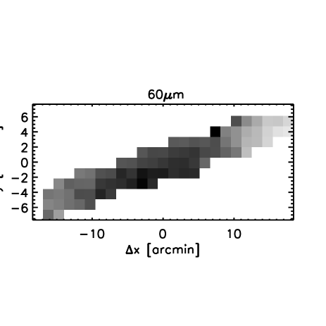
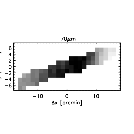
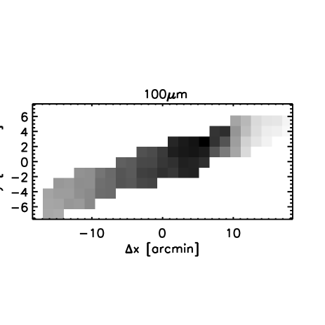
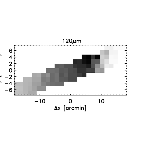
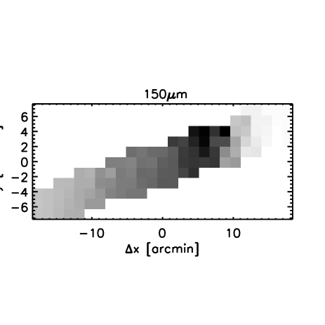
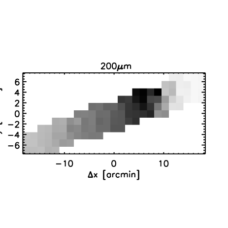
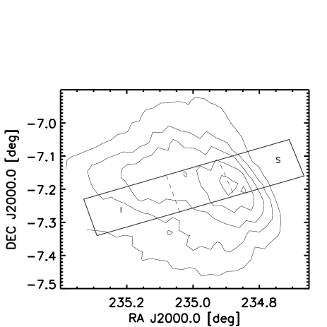
Figure 1: From top to bottom, from left to right: Emission at 60, 70, 100, 120, 150 and 200 $\mu$m smoothed to the angular resolution the 200 $\mu$m emission corresponding to the stripe region, which is overplotted on the 200 $\mu$m emission map corresponding to the square region. I and S labels respectively stands for the illuminated and shadowed regions separated by dashed lines from the rest of the stripe (see Sect. 2.4.1).

   

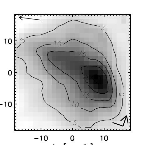
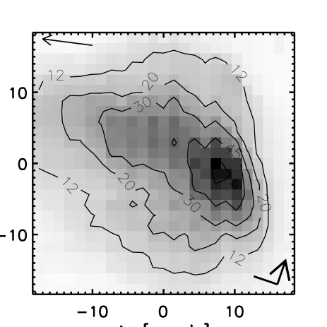
Figure 2: Left: ISOPHOT 100 $\mu$m emission smoothed to the angular resolution of the ISOPHOT 200 $\mu$m emission; Right: ISOPHOT 200 $\mu$m emission. Note the thin top-left arrow points to the Centaurus-Scorpius OB association. The NE axes are displayed on the bottom-right corner (arrow points to North).

Fig. 1 and 2 show the ISOPHOT emission maps of LDN 1780 for the stripe-like and the square regions, respectively. Maps in Fig. 2 were smoothed to the angular resolution of 200 $\mu$m ISOPHOT emission map (see Paper I). These maps have been zero-level calibrated following the procedure described in Sect. 2.4.

2.2 Near-infrared extinction

We built the extinction map of LDN 1780 following the method described in Cambrésy et al. (2002) using the 2MASS $H-K_{s}$ colour excess of 3400 stars in a $80^{\prime}\times 80^{\prime}$ field. The extinction is obtained following the expression:

$$A_{V}=\left(\frac{A_{H}}{A_{V}}-\frac{A_{K_{s}}}{A_{V}}\right)^{-1}\times(H-K_{s})+\mathcal{Z}_{\rm col}$$ (1)

where $(A_{H}/A_{V}-A_{K_{s}}/A_{V})^{-1}=15.87$ (Rieke & Lebofsky 1985) and $\mathcal{Z}_{\rm col}=-1.9$ mag. The zero point for the extinction calibration, $\mathcal{Z}_{\rm col}$, corresponds to an intrinsic star colour of $\overline{H-K_{s}}=0.12$ mag, measured outside the cloud. Any diffuse extinction in the field is therefore removed by construction. The extinction is obtained by taking the median value within adaptive cells that contain a constant number of 3 stars. This produces a map with a varying resolution, increasing with the star density. The resulting map is convolved with an adaptive kernel to obtain the final maps at the uniform resolutions of $4^{\prime}$ and $6^{\prime}$ (see Fig. 3). Although one can naïvely think this approach is equivalent to directly use an uniform grid of $4^{\prime}$ or $6^{\prime}$, it is fundamentally different. Because the ISM has small-scale structures, variations of the extinction within a cell are expected. The direct consequence of the sub-cell structures is that stars are not uniformly distributed within a cell, but are preferentially detected in the lower extinction region of a cell. In the classical method with large cells, the few stars detected at higher extinction do not contribute significantly to the colour median of a cell. The weight of the low-extinction part of a cell is increased and the extinction measurements are biased towards small values. In the adaptive method with only 3 stars, cells have the minimum size and the final 4 or $6^{\prime}$ resolution is obtained through a convolution. The weight of the low extinction region does not dominate anymore since these cells are smaller than at large extinction. Using adaptive cells and a convolution give a weight to the individual reddening measurements that is proportional to the surface of the voronoi cell defined by 3 stars (the voronoi cell for a single star represents all points equidistant of the central star to the surrounding objects). This technique integrates both the star colour and density, which optimises the extinction estimate by reducing the bias due to the inhomogeneous star distribution within a cell (see Cambrésy et al. 2005 for more details). The statistical uncertainties in the extinction maps are 0.4 mag and 0.5 mag for the $6^{\prime}$ and $4^{\prime}$ resolution, respectively. At these angular resolutions, the $6^{\prime}$ and $4^{\prime}$ extinction maps respectively reach maxima of 3.9 mag and 4.4 mag in the central region of LDN 1780.

           

Figure 3: Extinction map and contours in $A_{V}$ units. Pixel size of $4^{\prime}\times 4^{\prime}$. Coordinates [0,0] correspond to $\alpha_{2000}$=15^h40^m11.6^s and $\delta_{2000}$=-7^o12^′13.5^′′.

2.3 Additional data

In order to complement the ISOPHOT dataset of LDN 1780, the following additional data were included:

1. IRIS maps (Miville-Deschênes & Lagache 2005) at 25, 60 and 100 $\mu$m, with angular resolutions (noise levels in MJy sr^-1) of 3.8^′ (0.05), 4.0^′ (0.03) and 4.3^′ (0.06), respectively.

2. Carbon monoxide observations at 2.7 mm, (CO and ¹³CO) from LFHMIC95, with an angular resolution of 2.7^′. In particular we have used the velocity-integrated (line integrated) emission maps of CO (W₁₂) and ¹³CO (W₁₃).

3. H$\alpha$ surface brightness map, with an angular resolution of 6^′, belonging to the H-alpha Full Sky Map (Finkbeiner 2003). The absolute calibration of the composite H$\alpha$ emission map is based on the undersampled WHAM survey (1 deg spacing; 1 deg diameter top-hat beam). The error in a 40${}^{\prime}\times$40^′ H$\alpha$ emission map of LDN 1780 is $\sim$0.4 Rayleigh (1 Rayleigh=$\frac{10^{6}}{4\pi}$ $\gamma$ cm^-2 s^-1 sr^-1).

2.4 Data preparation

We have applied different analysis approaches for the data analysis of the stripe-like region and squared field data. In the remainder of this paper, we shall use the symbol $I_{\nu}$($\lambda$) (in $\mathrm{MJy\,sr^{-1}}$) to refer to the surface brightness, where $\lambda$=25, 60, 70 and 100, 120 and 200 $\mu$m corresponds to the reference wavelengths of the IRIS and ISOPHOT filterbands. A distinction between IRIS and ISOPHOT data will be noticed if necessary. $I_{\nu}({\mathrm{H}}\alpha)$ refers to the H$\alpha$ surface brightness. ${\Delta}I_{\nu}$($\lambda$) refers to the error at the reference wavelength $\lambda$.

2.4.1 Far-infrared emission correlations: stripe-like region

Following the analysis of Paper I, we have derived colour variations from the analysis of the correlations of $I_{\nu}(\lambda)$ ($\lambda<$200 $\mu$m) with $I_{\nu}(200)$ corresponding to the stripe-like region. As described in Paper I, any colour variation will result in a deviation from linearity in the correlations. The method offers some advantages (see Paper I for a detailed discussion). Slopes of correlations are direct measurements of the colour ratios and are independent of any emission offset; we therefore did not apply any zero-level correction to the stripe-like region. In addition, slopes are much more accurate than the absolute surface brightness, removing a significant amount of the random noise of individual pixels. In particular, when temperature variations are within the uncertainties for a certain region, the use all independent points improves the accuracy and the method applied is optimal.

All the stripe-like region data were obtained using ISOPHOT. Data corresponding to the C100 camera were smoothed to the angular resolution of the 2$\times$2 pixel C200 camera. Fig. 4 shows the correlations for the emissions at 60, 70 and 100, 120 versus emission at 200 $\mu$m. Correlations for two separated regions of LDN 1780 have been considered (see Fig. 1, bottom): a region in the shadow part of the cloud and a similar-in-size region in the illuminated side of the cloud, which faces the Galactic plane and the OB association. The instrumental noises of these emissions have been determined from the pixel to pixel response variations derived from the FCS measurements (see Table 2).

   

   

 

Figure 4: Surface brightness $I_{\nu}$($\lambda$) versus $I_{\nu}$(200) for wavelengths of 60, 70, 100, 120 and 150 $\mu$m. White and black circles respectively correspond to the illuminated region and shadowed region of LDN 1780. Straight lines that fit the data points are overplotted (see Sects. 2.4.1 and 3.1.1).

2.4.2 Map homogenisation: squared field

The maps of IRIS, ISOPHOT, the carbon monoxide lines as well as the H_α surface brightness map for the squared field have different angular resolutions. For a proper comparison the maps were smoothed to the worst angular resolution. For the analysis of far-infrared, extinction and molecular data, maps were smoothed to the angular resolution of the 100 $\mu$m IRIS map of 4.3^′ (corresponding to 0.14 pc for a distance of 110 pc). For a comparison with the H$\alpha$ surface brightness with FWHM$\approx$6^′, the maps were smoothed to mimic that angular resolution.

   

   

   

Figure 5: Top-left: IRIS 25 $\mu$m emission map; Top-right: IRIS 60 $\mu$m emission map; Middle-left: IRIS 100 $\mu$m emission map; Middle-right: ISOPHOT 200 $\mu$m emission map. All maps with angular resolution of 4.3^′. The NE axes (arrow points to North) are displayed on the bottom-right corner of each map. The thin and thick lines respectively correspond to the 1:1 and observed relations; Bottom-left: ISOPHOT 100 $\mu$m emission versus IRIS 100 $\mu$m emission. Note emission are not colour-corrected. The thin and thick lines respectively correspond to the 1:1 and observed relations; Bottom-right: ¹³CO(J=1-0) line integrated. Units of K Km s^-1.

In Fig. 5 the 25, 60 and 100 $\mu$m IRIS maps (see Fig. 5, top, middle-left) and 200 $\mu$m ISOPHOT map (see Fig. 5, middle-right) at the angular resolution of 4.3^′ are shown.

The median instrumental noise in $I_{\nu}(25)$, $I_{\nu}(60)$, $I_{\nu}(100)$ reported by Miville-Deschênes & Lagache (2005) is 0.05, 0.03 and 0.06 MJy sr^-1, respectively. For ISOPHOT, the pixel to pixel response variations derived from the FCS measurements (see Sect. 2.1) have been used to determine the instrumental noise. Table 2 shows the values of the instrumental noise at the different wavelengths for the observations. Data were smoothed to the $4.3^{\prime}$ angular resolution. When data from different instruments are combined we have also considered the relative errors between different filterbands. In Paper II we used a 5% between ISOPHOT filterbands and a pessimistic 30% for the relative error between IRIS 100 $\mu$m and the ISOPHOT 200 $\mu$m. Here, we have correlated the IRIS and smoothed 4.3^′ ISOPHOT 100 $\mu$m maps (see Fig. 5, bottom-left) to quantify this relative error in LDN 1780. We found an excellent correlation (Pearson correlation coefficient of PCC=0.97) between these maps and a relative error of only 1.6%. This value has been used as reference to derive the relative errors between IRIS and ISOPHOT filterbands assuming a 5% between different filterbands of the same instrument.

Table 2: ISOPHOT instrumental noise.

${\Delta}I_{\nu}(60)$	${\Delta}I_{\nu}(70)$	${\Delta}I_{\nu}(100)$	${\Delta}I_{\nu}(150)$	${\Delta}I_{\nu}(200)$	Remark
$[MJy\ sr^{-1}]$	$[MJy\ sr^{-1}]$	$[MJy\ sr^{-1}]$	$[MJy\ sr^{-1}]$	$[MJy\ sr^{-1}]$
0.4	0.35	0.3	0.55	0.5	stripe at $1.5^{\prime}$
-	-	0.45	-	0.76	square at $1.5^{\prime}$
-	-	0.16	-	0.27	square at $4.3^{\prime}$

2.4.3 Separation of the warm and cold components

The emission maps of the squared field in LDN 1780 at 25, 60, 100 and 200 $\mu$m show distinct morphologies that likely indicate variations in the abundance distribution across the cloud. Note, for instance, the different positions of the emissions peaks at different wavelengths in Fig. 5. See also Fig. 1 for intermediate wavelengths.

In order to distinguish between the different large dust grain components in LDN 1780 we have performed a first attempt to obtain the emission of the cold component at 100 $\mu$m (see Laureijs, Clark & Prusti 1991; Abergel et al. 1994), and at 200 $\mu$m (see Paper II) using the equation:

$${\Delta}I_{\nu}(\lambda)(x,y)=I_{\nu}(\lambda)(x,y)-I_{\nu}(60)(x,y)/\Theta(60,\lambda),$$ (2)

where ${\Theta}(60,\lambda)$ is the average colour $I_{\nu}(60)/I_{\nu}(\lambda)$ of LDN 1780. We have determined ${\Theta}(60,100)$=0.27 from the IRIS maps, which is the same value found by LFHMIC95 from previously realised IRAS data. Our value of ${\Theta}(60,\lambda)$ was determined using values of $I_{\nu}(100)$ below 90% of the peak of $I_{\nu}(100)$. We found ${\Theta}(60,200)$=0.13 using values of $I_{\nu}(200)$ below 90% of the maximum. The correlation between ${\Delta}I_{\nu}(100)$ and $I_{\nu}(200)$ has a PCC of 0.7.

The previous approach has been traditionally used to separate the BGs that are associated to the molecular regions and are free from VSG emission from the warm diffuse ISM. Although they were originally called warm and cold, these components separate two grain populations rather than two temperatures. In addition recent results obtained at longer wavelengths using far-infrared and submillimeter instruments indicate the presence of two temperature components of BGs, with temperatures of $\approx$16-22  K and $\sim$12 K, respectively, and different emissivities (Cambrésy et al. 2001, Papers I and II). The designation of warm and cold components is still used by the community to refer to this separation.

A second approach has been used to carry out the dust component separation. Before introducing this approach, we give a brief scientific justification for its use, which will be discussed in more detail in Sect. 3.6. Assuming a single BG component, the observed mean ratio $I_{\nu}(100)/I_{\nu}(200)$ would indicate a temperature of $\sim$17 K in the cloud, which is relatively high compared with other translucent clouds (see Paper I). Also, this temperature is significantly lower than the temperature of $\sim$13 K derived from the ${\Delta}I_{\nu}(100)/I_{\nu}(200)$ ratio using a modified black body with a power-law emissivity $\beta$=2. This discrepancy in temperature can be interpreted as due to the presence of two BG component instead of a single one. This could explain other findings in the cloud. It is observed that the 25 $\mu$m emission resembles properties of both the 12 and 60 $\mu$m emission maps. In addition, the average colour $\Theta(60,100)$=0.27 is relatively high with respect to the standard value in the ISM of $\Theta(60,100)$=0.21. LFHMIC95 suggested that the high ratio $\Theta(60,100)$ in LDN 1780 might be due to a high contribution of VSGs, but could be alternatively interpreted as due to the presence of a warm component of BGs. The enhanced stellar radiation field in LDN 1780 (LFHMIC95, THML95) due to the Galactic plane and a close OB association could produce that the warm and cold components present relatively high temperatures compared with those found in Cambrésy et al. (2001), Papers I and II. A significant contribution to the emission at 60 $\mu$m from warm BGs is therefore expected. The 25 $\mu$m emission, which presents a high S/N ratio, becomes the suitable template of the VSG emission.

Hereinafter, when referring to the emission of the warm and cold components we respectively use the superscripts $w$ and $c$. We determined the emission of the cold component at an intermediate wavelength (60, 100 and 200 $\mu$m) from the following equation:

$$I^{c}_{\nu}(\lambda)(x,y)=I_{\nu}(\lambda)(x,y)-c(\lambda,25)\times I_{\nu}(25)(x,y),$$ (3)

where $c(\lambda,25)$ is a constant value derived from the correlation $I_{\nu}(\lambda)$-$I_{\nu}(25)$. It corresponds to the slope of this correlation, i.e. $I_{\nu}(\lambda)$/$I_{\nu}(25)$, for values of $I_{\nu}(\lambda)$ below the 90% of its maximum. This is performed to reject out possible outliers in the emission maxima surroundings.

In order to determine the emission of the warm component at wavelengths $\lambda=$25, 60 and 100 $\mu$m we applied the equation:

$$I^{w}_{\nu}(\lambda)(x,y)=I_{\nu}(\lambda)(x,y)-w(\lambda,200){\times}I^{c}_{\nu}(200)(x,y),$$ (4)

where $w(\lambda,200)$ is the ratio $I_{\nu}(\lambda)$/$I^{c}_{\nu}(200)$. We have simply used $I_{\nu}(200)$ instead of $I^{c}_{\nu}(200)$ when determining $I^{w}_{\nu}(25)$.

Note this second approach provides emission maps at wavelengths 60, 100 and 200 $\mu$m for the cold component. The 100 and 200 $\mu$m emission maps will be used to derive colour temperature and optical depth maps in the Sections 3.2.2 and 3.3, respectively. For the warm component emission maps at 25, 60 and 100 $\mu$m are obtained. The latter two maps have been used to determine the colour temperature and optical depth of the warm component (see sections 3.2.3 and 3.3, respectively).

2.4.4 Zero level calibration

We have fixed to zero the minimum value of $I^{c}_{\nu}(100)$ in the field of view of ISOPHOT. The region is representative of the local background for LDN 1780. Then, the pixel-pixel correlations of $I^{c}_{\nu}(60)$ with $I^{c}_{\nu}(100)$ and $I^{c}_{\nu}(200)$ with $I^{c}_{\nu}(100)$ where used to derive the offsets of the emissions at 60 and 100 $\mu$m with respect the emission at 200 $\mu$m. We have estimated an error of ${\Delta}I^{c}_{\nu}(200)$=1 MJy sr^-1 due to the zero level uncertainty.

For the warm component we have fixed the minimum of $I^{w}_{\nu}(100)$ to zero. Then, the zero levels of the emissions at 25, and 60 $\mu$m and their corresponding errors were determined from the pixel-pixel correlations with the corrected $I^{w}_{\nu}(100)$. We have computed an error at the reference wavelength of 100 $\mu$m of ${\Delta}I^{w}_{\nu}(100)$=0.15 MJy sr^-1 due to the zero level uncertainty.

We were consistent with these definitions for the zero level calibration when applying the method described in the previous section, i.e, when removing the emissions at 25 and 200 $\mu$m emissions. We used the zero-level errors together with the relative errors between filterbands and the errors due to the instrumental noise when computing the temperature errors and the optical depth errors in the next sections.

3 Physical properties of the warm and cold components

3.1 Far-infrared emission

3.1.1 Striped region

We have determined the colour variations along the stripe-like region, in the illuminated and shadowed sides (see Fig. 1, bottom). For both sides, the correlations $I_{\nu}(\lambda)-I_{\nu}(200)$ shown in Fig. 4 present a linear behave within the scatter at wavelengths of 120 and 150 $\mu$m. This is described as unimodal behave in Paper I. At shorter wavelengths it is observed that each correlation is bimodal for the shadowed region: the colour variation is modelled by two connected linear ramps with a wavelength dependent turnover point. The observed flattening in the emissions towards higher 200 $\mu$m emission indicates a decrease in the colour ratio at higher column densities.

The slopes of the correlations for the unimodal and bimodal cases are determined from a least-squares linear fit. The regression fits are overplotted on the correlations in Fig. 4 and the slopes are listed in Table 3. $Slope_{1}$ and $Slope_{2}$ stand for the slope values of the correlations before and after the turnover emission point.

Table 3: Slopes in the regressions of the striped region observed using ISOPHOT. Uncertainties in the slopes correspond to statistical variations.

Region	$\lambda_{ref}$	Slope1	Slope2
	($\mu$m)
Shadowed	60	0.10$\pm$0.02	0.00$\pm$0.02
	70	0.19$\pm$0.01	0.10$\pm$0.06
	100	0.40$\pm$0.02	0.3$\pm$0.1
	120	0.55$\pm$0.01	-
	150	0.910$\pm$0.007	-
	200	1
Illuminated	60	0.118$\pm$0.009	-
	70	0.255$\pm$0.009	-
	100	0.48$\pm$0.01	-
	120	0.629$\pm$0.007	-
	150	0.89$\pm$0.01	-
	200	1	-

3.1.2 Squared region

We have determined the emission maps of the warm and cold components using the second approach described in Sect. 2.4.3. Emission maps of the warm component at 60 and 100 $\mu$m are shown (see Fig. 6 top-left and top-right, respectively). Emission maps of the cold component at 100 and 200 $\mu$m are shown (see Fig. 6 bottom-left and bottom-right, respectively). The Pearson correlation coefficients of the different correlations are listed in Table 4. The number of independent pixels (N_ip) used in the computation is also tabulated. The PCCs corresponding to the warm and cold components individually are generally better than the PCCs of the full emissions.

Table 4: Pixel-pixel correlations of the far-infrared emission before component separation (all), and for the warm and cold component. $PCC$ refers to the Pearson correlation coefficient and $N_{ip}$ corresponds to the number of independent pixels. Between brackets the results for the region with $I^{c}_{\nu}(200)\geq$ 9 MJy sr^-1.

	$I_{\nu}(25)$ vs $I_{\nu}(60)$		$I_{\nu}(60)$ vs $I_{\nu}(100)$			$I_{\nu}(100)$ vs $I_{\nu}(200)$
	all	warm	all	warm	cold	all	cold
$N_{ip}$	64	64	64	64	64(31)	64	64(31)
$PCC$	0.88	0.92	0.96	0.99	0.93(0.88)	0.98	0.98(0.97)

   

   

Figure 6: Top-left: Contours in MJy sr ^-1 corresponding to the 60 $\mu$m emission from the warm component; top-right: 100 $\mu$m emission from the warm component; bottom-left: 100 $\mu$m emission from the cold component; bottom-right: 200 $\mu$m emission from the cold component.

3.2 Colour temperature

3.2.1 Average colour temperatures in the illuminated and shadowed sides

We have determined the average colour temperatures in the shadowed and illuminated sides of LDN 1780 from the corresponding colour-corrected slope of correlation $I_{\nu}(150)-I_{\nu}(200)$, assuming that the spectral energies distributions are well represented by a modified black body with power-law emissivity $\beta=2$ as performed in Paper I. We have overplotted the fitted modified black body on the spectral energy distributions (SEDs) of the shadowed region (see Fig. 7, left) and illuminated region (see Fig. 7, right). In the shadowed region we observed a bimodal behave, with a flattening in the correlations $I_{\nu}(\lambda)-I_{\nu}(200)$ at higher 200 $\mu$m emission. Two modified black bodies with a power-law emissivity $\beta=2$ have been considered: one which fits to the $I_{\nu}(150)-I_{\nu}(200)$ correlation; other one that fits to the $I_{\nu}(120)-I_{\nu}(200)$ correlation, which is representative of the denser region (using $slope_{2}$ at 120 $\mu$m of Table 3). The colour temperatures of the fits are 16.1 and 15.5 K, respectively. It is observed that the fitted models for the shadowed region reproduce within the errors the entire SED for both datasets, and therefore no significant excess is observed at any wavelength apart from 60 $\mu$m in the low density region. An uncertainty in the temperature of 0.2 K has been determined from the statistical and responsivity variations.

In the illuminated region a colour temperature of 15.9$\pm$0.2 K is obtained from the colour ratio derive from 150 and 200 $\mu$m emissions. It is observed an emission excess at all wavelengths including 100 and 120 $\mu$m with respect the fitted modified black body with T=15.9 and $\beta=2$.

   

Figure 7: Left: SED in the shadowed region of LDN 1780. Two modified black bodies are overplotted: one with the colour temperature fitted to the $I_{\nu}(150)-I_{\nu}(200)$ correlation; the other one fitted to the $I_{\nu}(120)-I_{\nu}(200)$ representative of the denser region; Right: SED in the illuminated region.

3.2.2 Colour temperature of the cold component

A colour temperature map of the cold component (see Fig. 8) was determined from the $I^{c}_{\nu}(100)$ and $I^{c}_{\nu}(200)$ maps that were obtained using the second approach described in Sect. 2.4.3. For each independent pixel, the emissions were colour-corrected and fitted to a modified black body with $\beta$ = 2. The temperature map might present a small gradient with temperatures increasing from $\approx$15.8 to 17.3 K along the NW-SE axis for the region enclosed by the 9 MJy sr^-1 isophote of $I^{c}_{\nu}(200)$ (see Fig. 8), outside which the temperature errors significantly increase. The mean temperature is 16.3 K.

The error in temperature is determined from the instrumental errors of the IRIS 100 $\mu$m and ISOPHOT 200 $\mu$m filter-bands, as well as the relative errors and the zero-level uncertainty (see Sect. 2.4.4). The errors in temperature are $\pm$0.5 K in the area closed by the isophote $I^{c}_{\nu}(200)$ above 9 MJy sr^-1. The temperature errors at lower emissions increase to few  K and we have not included them in our analysis.

           

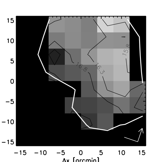
Figure 8: Colour temperature map and contours (in steps of 0.5 K) of the cold component. Pixel size of $4^{\prime}\times 4^{\prime}$. The uncertainties $\pm$0.5 K. The white thick contour marks the 9 MJy sr^-1 isophote of $I^{c}_{\nu}(200)$.

3.2.3 Colour temperature of the warm component

The colour temperature map of the warm component was determined from the $I^{w}_{\nu}(60)$ and $I^{w}_{\nu}(100)$ maps. The carriers in the wavelength range between 60 and 100 $\mu$m are generally VSGs and “classical” BGs. However, $I^{w}_{\nu}(60)$ was built up to be free from VSGs and cold BGs (see Sect. 2.4.3). For each independent pixel, emissions were colour-corrected and fitted to a modified black body with $\beta$ = 2. The mean colour temperature is 25 K. We determined errors in temperature of $\pm$1 K with the same criteria applied for the cold component but using the errors in the 60 and 100 $\mu$m emissions. When assuming a lower value of $\beta$, temperature increases. For example, for $\beta$=1, the colour temperature of the warm component would be 30$\pm$1.5 K.

3.3 Optical depths of the warm and cold component

The optical depth of the cold component at 200 $\mu$m (see Fig. 9, left) has been obtained using the relation $\tau^{c}_{\nu}(200)(x,y)$=$I^{c}_{\nu}(200)(x,y)/B_{\nu}(T)$, where the Planck function $B_{\nu}(T)$ is determined at 200 $\mu$m, using the colour temperature $T$ derived in Sect. 3.2.2. The map presents a peak at 7.3${}^{+1.1}_{-0.9}\times 10^{-4}$, whose location is in agreement with the maxima of $I^{c}_{\nu}(200)$ and $A_{V}$. The mean errors are ${\Delta}\tau^{c}_{\nu}(200)=^{+16\%}_{-13\%}$.

The optical depth of the warm component at 100 $\mu$m, $\tau_{\nu}^{c}(100)$ (see Fig. 9, right), has been similarly obtained from $I^{c}_{\nu}(100)$ and the Planck function at 100 $\mu$m and temperatures derived in the previous section. We have computed an error of ${\Delta}\tau^{w}_{\nu}(100)=^{+30\%}_{-20\%}$. The optical depth at 100 $\mu$m can be converted into optical depth at 200 $\mu$m by dividing $\tau^{w}_{\nu}(100)$ by $(200/100)^{2}$ assuming $\beta=2$. We note that the optical depth of the warm component is few tens lower than the optical depth of the cold component.

   

Figure 9: Left: Image of $\tau^{c}_{\nu}(200)$ and contours overplotted in units of 10^-4. Contour of $I^{c}_{\nu}(200)=$ 9 MJy sr^-1 is overplotted; Right: Image of $\tau^{w}_{\nu}(100)$ and contours overplotted in units of 10^-4. Note $\tau^{w}_{\nu}(100)$ can be converted to $\tau^{w}_{\nu}(200)$ dividing by 4 (see text).

3.4 The extinction-infrared relation: an estimation of the emissivity of the warm component

The correlation $I^{c}_{\nu}(200)-A_{V}$ (PCC=0.76) presents a higher scatter for low emission with $I^{c}_{\nu}(200)$ below $\approx$ 10 MJy sr^-1. At this low emission level there are some satellite $A_{V}$ peaks surrounding the $A_{V}$ maximum that correlate well with $\tau^{w}_{\nu}(100)$, i.e., the infrared tracer of the column density of the warm component (see figures 3 and 9, right). This indicates that $A_{V}$ also gauges the column density of the warm component in the external regions. Therefore the total extinction can be written as the sum the warm and cold components (see also Cambrésy et al. 2001):

$$A_{V}=A^{c}_{V}+A^{w}_{V}$$ (5)

The extinction of the warm component $A^{w}_{V}$ can be related to $\tau^{w}_{\nu}(100)$ using the next expression:

$$A^{w}_{V}=\tau^{w}_{\nu}(100)/\frac{\tau^{w}_{\nu}(100)}{A^{w}_{V}}$$ (6)

Assuming that the ratio $\frac{\tau^{w}_{\nu}(100)}{A^{w}_{V}}$ is constant, it is possible to derive $A^{w}_{V}$ from Eq. 6 and subtract it from Eq. 5 to determine $A^{c}_{V}$.

The value of $\frac{\tau^{w}_{\nu}(100)}{A^{w}_{V}}$ has been obtained maximising the correlation between $\tau_{\nu}^{c}$ and the residual $A^{c}_{V}{\equiv}A_{V}-A^{w}_{V}$. We obtained $\frac{\tau^{w}_{\nu}(100)}{A^{w}_{V}}\approx$1 10^-4 mag^-1, which corresponds to $\frac{\tau^{w}_{\nu}(200)}{A^{w}_{V}}$=0.25 10^-4 mag^-1 for $\beta$=2. This value implies a range of $A^{w}_{\nu}$ between 0.01 and 1.3 mag. For $\beta$=1, it is derived that $\frac{\tau^{w}_{\nu}(100)}{A^{w}_{V}}=0.5\ 10^{-4}$ mag^-1. Fig. 10 (right) shows the $I^{c}_{\nu}(200)-A^{c}_{V}$ correlation with PCC=0.80. It is found that PCC=0.85 if considering only values of $I^{c}_{\nu}(200)$ above 9 MJy sr^-1.

An averaged ratio $I^{c}_{\nu}(200)/A^{c}_{V}$ = 12.1$\pm$0.7 MJy sr^-1 mag^-1 is derived from the $I^{c}_{\nu}(200)-A^{c}_{V}$ correlation using the bisector method (Isobe et al. 1990). The slope is the same when using $A_{V}$ instead of $A^{c}_{V}$. It is interesting to note that the zero level calibration established in Sect. 2.4.4 is in agreement with the origin of the $I^{c}_{\nu}(200)-A^{c}_{V}$ correlation. Note that if adding an offset of 0.3 mag to $A^{c}_{V}$ (see Fig. 10, right), the $I^{c}_{\nu}(200)-A^{c}_{V}$ will pass though the origin (i.e., $I^{c}_{\nu}(200)(A^{c}_{V}=0)$=0). This offset of 0.3 mag is consistent with the scatter in the relation $I^{c}_{\nu}(200)-A^{c}_{V}$ and also with the uncertainty in $A^{c}_{V}$ (see Sect. 2.2).

From the correlation $\tau^{c}_{\nu}(200)-A^{c}_{V}$ we have derived that $\tau^{c}_{\nu}(200)/A^{c}_{V}=(2.0\pm 0.2)10^{-4}$ mag^-1, which is similar to the value in the DISM, but few times lower than the values found in other translucent regions (see Paper I).

   

Figure 10: Left: $I^{c}_{\nu}(200)$ versus $A_{V}$; Right: $I^{c}_{\nu}(200)$ versus $A^{c}_{V}$. Solid lines show the corresponding least-squares fitting, and dotted lines indicate the corresponding upper and lower 3$\sigma$ limits.

3.5 Relations of the warm and cold components with the HI excess emission, $W_{12}$ and $W_{13}$

We have observed that the warm component is located in the illuminated side of LDN 1780 as well as the HI excess emission (Mattila & Sandell 1979).

The monoxide line integrated $W_{12}$ and $W_{13}$ do not correlate with the warm component. The correlations with the cold component are very good (see Fig. 11 and Table 5). The correlation between $W_{13}$ and $\tau^{c}_{\nu}(200)$ and also with $I^{c}_{\nu}(200)$ are especially good with PCC=0.96. The morphologies of $\tau^{c}_{\nu}(200)$ and $W_{13}$ are very similar (see Figs. 5 and 9, left).

The ordinary least squares bisector method has been used to determine $\tau^{c}_{\nu}(200)/W_{13}$ from the correlation $\tau^{c}_{\nu}(200)-W_{13}$. We obtained that $\tau^{c}_{\nu}(200)/W_{13}=(5.2\pm 0.2){\times}10^{-4}$ K^-1 Km^-1 s. An offset of ${\Delta}\tau^{c}_{\nu}(200)=(0.91\pm 0.07){\times}10^{-4}$ is obtained.

 

Figure 11: Correlation $W_{13}-\tau^{c}_{\nu}(200)$. Mean errors are indicated. A total of 34 independent pixels with size $6^{\prime}\times 6^{\prime}$ is shown.

Table 5: Correlations of $W_{13}$ and $W_{12}$ with $I_{\nu}(200)$, $I^{c}_{\nu}(200)$ and $\tau^{c}_{\nu}(200)$. $PCC$ refers to the Pearson correlation coefficient and $N_{ip}$ corresponds to the number of independent pixels. $W_{13}$ and $W_{12}$ are positive values. Between brackets the results for the region with $I^{c}_{\nu}(200)\geq$ 9 MJy sr^-1.

	$W_{13}$			$W_{12}$
	$I_{\nu}(200)$	$I^{c}_{\nu}(200)$	$\tau^{c}_{\nu}(200)$	$I_{\nu}(200)$	$I^{c}_{\nu}(200)$	$\tau^{c}_{\nu}(200)$
$N_{ip}$	34	34(26)	34(26)	52	52(31)	51(31)
$PCC$	0.79	0.96(0.95)	0.96(0.96)	0.77	0.82(0.69)	0.74(0.63)

3.6 Discussion

3.6.1 Separation of the warm and cold components

LFHMIC95 already pointed out that the profile (along the direction of the Upper Scorpius OB association) of 25 $\mu$m emission in LDN 1780 shows a different distribution with respect to the 12 and 60 $\mu$m emissions. In the classical picture, this could be interpreted as due to a stronger emissivity of the VSGs, which mostly emit at 60 $\mu$m. We have alternatively interpreted that the spectra energy distribution in LDN 1780 is mostly due to the existence of cold BGs together with warm BGs and VSGs illuminated by an enhanced local interstellar radiation field. The warm and cold components have high temperatures compared to other moderate density regions (see Paper I) and consequently the bulk of their emissions is displayed towards shorter wavelengths. In the illuminated side of the stripe, it is observed emission excess at 100 and 120 $\mu$m over a modified black body with the colour temperature derived from the $I_{\nu}(150)-I_{\nu}(200)$ correlation. This excess at such long wavelengths can not be due to VSGs and supports the existence of an additional BG component.

In previous studies, the 60 $\mu$m emission has been used as template to derive the excess emission at 100 $\mu$m (Laureijs, Clark & Prusti, 1991; Abergel et al. 1994) and also 200 $\mu$m (see Paper II). The correlation ${\Delta}I_{\nu}(100)-I_{\nu}(200)$ (PCC=0.70) derived from our first approach is not as good as the $I^{c}_{\nu}(100)-I_{\nu}(200)$ correlation (PCC=0.98) obtained from the second approach (see Sect. 2.4.3). Different mean colour temperatures are derived, with $\sim$13 K and $\sim$16 K for the first and second approaches, respectively. The low temperature of $\sim$13 K is likely due to the fact that $I_{\nu}(60)$ contains not only emission from VSGs but also from warm BGs. The second approach to separate the warm and cold components is intended to sort out this problem. The S/N of the emission at 25 $\mu$m is high enough to be used as template of the VSG component.

The goodness of the second approach to disentangle the different dust components is supported by the good agreement between the temperatures obtained for the squared field map of the cold component and the shadowed side of the stripe-like region. It is also supported by the very good correlation between W₁₃ and $\tau^{c}_{\nu}(200)$. When using the first approach the optical depth of the cold component is not so well correlated with W₁₃. The ${\Delta}I_{\nu}(100)-I_{\nu}(200)$ correlation is not as good as $I^{c}_{\nu}(100)-I_{\nu}(200)$. In addition, the warm component presents a distribution which is similar to the HI excess emission, facing the illuminated side of the cloud

Regarding the properties of the warm component (see Sects. 3.2.3 and 3.3) it is difficult to derive its emissivity. We have found a ratio $\tau\nu^{w}(100)/A_{V}$ which is significantly low. The temperature could be also somehow overestimated since it could be that $I_{\nu}(200)$ contains some contribution of the warm component, which is not considered in Eq. (4). However, the mentioned agreement between the temperature derived for the stripe in the shadowed region and temperature in the corresponding region in the squared field supports the consistency of our results.

3.6.2 Properties of the cold component

The cold component exhibits a temperature of $\approx$16 K, which is higher than expected at the UV-shielded densities of 10²-10³ cm^-3. This requires either an extra heating rate through the cloud or a change in the properties of the grains with respect those of the DISM.

The average value of $I_{\nu}(200)$/A_V=12.1$\pm$0.7 MJy sr^-1 mag^-1 of the cold component in LDN 1780 is below the value of the diffuse interstellar medium with $I_{\nu}(200)$/A_V=21.1 MJy sr^-1 mag^-1 and T=17.5 K, and also below the values of the moderate density regions of the sample in Paper I. These regions are generally colder than LDN 1780 and have a cold component with an enhanced far-infrared emissivity.

The average ratio $\tau^{c}_{\nu}(200)/A^{c}_{V}$=(2.0$\pm$0.2)$\times$10^-4 mag^-1 is slightly lower than the value of the DISM ($\tau^{c}_{\nu}(200)/A_{V}$=2.4$\times$10^-4 mag^-1) and the same than in the warmer (T=18.9$\pm$0.7 K) G90.7+38.0 (2.0$\pm$0.8)$\times$10^-4 mag^-1) (see Paper I). When considering values of independent pixels, we find a variation in $\tau^{c}_{\nu}(200)/A^{c}_{V}$ from 1 10^-4 mag^-1 to 3 10 ^-4 mag^-1 for temperatures of 17.3 and 15.8  K, respectively. A small enhancement in the emissivity of the cold component is therefore observed. This could be related to grain coagulation as observed in other translucent clouds (see Paper I).

3.6.3 Properties of the warm component

The temperature of the warm component of 25$\pm$1 K ($\beta=2$) is higher than the average value of the DISM (17.5 K). The warm component, which is surrounding the cold component, it is certainly affected by the anisotropy of the radiation field. The maximum of the far infrared emission of the warm component is located in the illumination side of the cloud.

For $\beta$=2 we obtained $\tau^{w}_{\nu}(200)/A^{w}_{V}$=0.25$\times$10^-4 mag^-1. This value is significantly lower than the values for the cold component as well as the DISM and G90.7+38.0. All these regions are significantly colder than the warm component in LDN 1780. This supports that the properties of the dust grains of the warm component are different from those of the DISM as well as the cold component. This could be result of the enhanced radiation field in the surroundings of LDN 1780 with respect the DISM. The observation of the emission of all the area LDN 1780 at intermediate wavelengths between 100 and 200$\mu$m would help to a better extraction of the warm component.

Note that $\beta$ could be different for the warm and cold components (see also discussion in Paper II). An unrealistic value of $\beta$=1 for the warm component implies that $\tau^{w}_{\nu}(100)/A^{w}_{V}$ decreases $\sim$50%. If $\beta\sim$1.5, then T$\sim$27 K and the ratio $\tau^{w}_{\nu}(100)/A^{w}_{V}$ drops $\sim$20% with respect to the value for $\beta$=2. A further investigation is out of the scope of the data presented here.

4 Ionisation process

4.1 Relation $A_{V}-I_{\nu}({\mathrm{H}}\alpha)$

The H$\alpha$ emission in LDN 1780 (see Fig. 12, left) varies between $\sim 1$ and 4 Rayleigh, and its error is $\sim$0.4 Rayleigh (Finkbeiner 2003). The extinction $A_{V}$ correlates very well with the H$\alpha$ emission, with a Pearson correlation coefficient of 0.71 (see Fig. 12, right). There is a linear relation between the H$\alpha$ emission and $A_{V}$ that remains till $A_{V}\sim$2 mag, and then flattens. The correlation is observed in regions with an abundant molecular gas content, which is surprising since the UV radiation field from the Galactic plane and the Sco-Cen OB association cannot come in through so deep (see Sect. 4.2.1).

Such a good correlation between the H$\alpha$ emission and the extinction in LDN 1780 strongly suggests that the ionised gas and the dust share a significant emitting volume and are quite uniformly mixed within it. The flattening in the H$\alpha$ emission at high $A_{V}$ ($\sim$2 mag) is likely result of dust extinction (see Fig. 12, right). It is therefore suitable to correct the observed H$\alpha$ emission $I_{\nu,obs}({\mathrm{H}}\alpha$) from extinction using the following equation:

$$I_{\nu}({\mathrm{H}}\alpha)=\frac{I_{\nu,obs}({\mathrm{H}}{\alpha})~{}\tau({\mathrm{H}}{\alpha})}{(1-e^{-\tau({\mathrm{H}}{\alpha})})}$$ (7)

The optical depth at the wavelength of H$\alpha$ is obtained from our near-infrared extinction map and the Cardelli, Clayton & Mathis (1989) extinction law which gives $A_{{\mathrm{H}}\alpha}/A_{V}=0.72$ so that $\tau({\mathrm{H}}\alpha)=2.5\log e\times 0.72\times A_{V}$. In the surroundings of the cloud, with $\tau({\mathrm{H}}{\alpha})\rightarrow 0$, the equation (6) gives $I_{\nu}({\mathrm{H}}\alpha)\approx I_{\nu,obs}({\mathrm{H}}\alpha)$; toward the peak of the cloud $I_{\nu}({\mathrm{H}}\alpha)\approx\tau({\mathrm{H}}{\alpha})\ I_{\nu,obs}({\mathrm{H}}\alpha)$.

The $A_{V}-I_{\nu}({\mathrm{H}}\alpha)$ plot, with the extinction-corrected H$\alpha$ is shown in Fig. 12 (right). Using a ordinary least squares bisector method (Isobe et al. 1990), we obtained a ratio $I_{\nu}({\mathrm{H}}\alpha)/A_{V}$=2.2$\pm$0.1 R mag^-1. This is twice the value of $I^{obs}_{\nu}({\mathrm{H}}\alpha)/A_{V}$. Note there is an offset in the relation with $I_{\nu}({\mathrm{H}}\alpha)$=1.4$\pm$0.15 R at $A_{V}=0$ mag.

   

Figure 12: Left: $I_{\nu}({\mathrm{H}}\alpha)$ contours (before correction from extinction) in Rayleigh; Right: $I_{\nu}({\mathrm{H}}\alpha)$ before (open circles) and after (filled circles) correction from extinction versus $A_{V}$. A total of 36 independent pixels with size of $6^{\prime}\times 6^{\prime}$. Mean error bars are also indicated.

4.2 Enhanced ionisation rate

The disk-like distribution of emitting gas in the Galaxy produces an emission $I_{\nu}({\mathrm{H}}\alpha)\approx\frac{1}{sin(b)}$ Rayleigh (Reynolds 1984), which corresponds to 1.7 R at the latitude of LDN 1780.

The observed relation between $I_{\nu}({\mathrm{H}}\alpha)$ and $A_{V}$ indicates that the ionisation and recombination processes are even produce in very deep regions of the cloud, with optical extinctions of $\sim$2 mag. This is likely due to a source of ionisation that can penetrate much deeper into the cloud than the UV and the X-ray radiations and produces a nearly uniform ionisation rate in the cloud.

The observed ratio $I_{\nu}({\mathrm{H}}{\alpha})/A_{V}$ gives us the possibility to estimate the ionisation rate from the following equation:

$$\xi\approx\frac{\frac{I_{\nu}(H_{\alpha})}{A_{V}}}{\frac{N(H+H_{2})}{A_{V}}}$$ (8)

which results to be $\sim$10^-16 $\gamma$ s^-1. We have used $N(H+H_{2})/A_{V}$ = $1.87\times 10^{21}$ mag^-1 cm^-2 (Bohlin, Savage & Drake 1978). Although this corresponds to a very high ionisation rate for the intermediate density cloud LDN 1780, it worth noting it is only a lower limit obtained by assuming that every collision with an high energy particle yield a H$\alpha$ photon emission. Other clouds in the LDN 134 like LDN 169, LDN 183 and LDN 134 also present H$\alpha$ emission. The origin of the ionisation source is discussed in the next sections.

4.2.1 Influence of the X-ray and UV radiation fields

LDN 1780 as well as LDN 134, LDN 183 and LDN 169 are likely influenced by an anisotropic radiation field (THLM95, LFHMIC95). The southern sides of these clouds face the nearby UV sources $\zeta$ Oph (an O9.5V star at a distance of 140 pc from the Sun) and the Upper Scorpius OB association.

LFHMIC95 studied the variation of the dust and molecular gas tracers along a line parallel to the direction of the UV radiation field (assumed toward Upper Scorpius OB association) crossing the centres of LDN 1780 and LDN 134. They pointed out some differences between these clouds. For LDN 1780: i) no detection of dense and opaque clumps is observed, although THLM95 found a weak emission of C¹⁸O, ii) the emission is significantly brighter at 25, 60 and 100 $\mu$m emission compared to LDN 134 (also LDN 183); iii) the 60 and 100 $\mu$m profiles are asymmetric (as in LDN 134), but similar, and peak at the same position as the carbon monoxide lines, while in LDN 134 there is an offset for the W(¹³CO); iv) $I_{\nu}(60)/I_{\nu}(100)$ and $I_{\nu}(12)/I_{\nu}(25)$ decreases toward the shadow side, while in LDN 134 they are either nearly constant or present a decrease toward higher densities; v) the CO temperature peak is highly symmetric, contrary to LDN 134; vi) the lines are narrower on the shadow side.

THLM95 suggested that only the external region of LDN 1780 might be affected by the local radiation field. They estimated that the radiation field in the illuminated side of LDN 1780 could few (2 or 3) times higher than the average radiation field at its Galactic latitude because of the presence of the OB association. THLM95 concluded the asymmetric UV illumination from the Scorpius-Centaurus association and from the Galactic plane has influenced the morphology of LDN 1780, resulting in the offset of the HI emission maximum, the blue-shifted (out-flowing) molecular gas envelope and the enhancement of the VSG abundance toward the side facing the Galactic plane. THLM95 claim that the offset found between the radiation temperature peaks of CO and ¹³CO and the comet-like morphology cannot be explained by the UV asymmetry. They concluded from the study of the morphologies of CO(J=1-0) and ¹³CO(J=1-0) that the offset between the maximum of the CO temperature peak and the geometrical centre can be explained as result of a shock front that passed through the cloud. The core of ¹³CO and the evaporating lower density envelope of gas pointing to NE correspond to the “head” and the “tail” of the cometary nebula, respectively (see next Sect.).

The maps of H$\alpha$ emission and $A_{V}$ show a good correlation, and no asymmetry evidence is observed between the shadow and illuminated sides. The observe H$\alpha$ enhancement is entirely related to LDN1780. We also observe that H$\alpha$ emission is present in the other clouds of the LDN 134 complex. However, LDN 1780 is the only cloud of the LDN 134 complex where ERE emission has been reported (Chlewicki & Laureijs 1987). Smith & Witt (2002) have interpreted the ERE in LDN 1780 as result of photoluminescence of silicon nanoparticles. They observed a relatively high quantum efficiency of the ERE process ($\sim$13%) as well as a long wavelength emission peak at 7000 Å. They argued that given the relatively high electron density and low UV photon density within the cloud in comparison with the DISM, the overall ionisation equilibrium tends more towards neutrality, and then the silicon nanoparticles are predominantly neutral, with an increment in the abundance of the largest particles, and then the overall quantum efficiency increases and the emission peak shifts to longer wavelengths. We have checked the H$\alpha$ emission maps and far-infrared emission of the 23 objects (DISM, LDN1780, reflection nebulae, HII regions) in the sample of Smith & Witt (2002) finding that there are only few of them with a clear counterpart in H$\alpha$. LDN 1780 is one of the few of them with a correlation between H$\alpha$ and far-infrared emission. We have also noticed that other clouds of the LDN 134 complex as the dense LDN 183 present H$\alpha$ in regions with a very low emission at 12 and 25 $\mu$m.

We conclude that the asymmetry of the radiation field is mainly affecting the warm component, which mostly contain warm BGs. The warm component is likely associated to the HI excess emission and it is surrounding the cold component (see Figure 6). The cold component, consisting of cold big dust grains, is well shielded from the UV radiation. The observation of H$\alpha$ emission at high column densities where CO emission is also observed supports the existence of a ionisation flux that can penetrate very deep into the cloud reaching the inner regions of it with $A_{V}\approx$2 mag. The UV radiation field from the Galactic plane and the OB association significantly decreases for $A_{V}\approx$0.3-0.5 mag and can not explain the observed CO and H$\alpha$ emissions. The X-rays dominates the cosmic ionisation for smaller column densities. Therefore, both ionisation sources cannot give account of the observed ionisation rate in LDN 1780 and can be rejected out.

4.2.2 Is it possible that the H$\alpha$ emission in LDN 1780 has been produced by a shock?

THLM95 pointed out the importance of a shock front of $\sim$10 Km s^-1 in the morphology of LDN 1780. Based on the idea of de Geus et al. (1989), THLM95 suggested that an expanding HI shell originated from the Scorpius-Centaurus OB association could be eventually fragmented forming clumps that were reached by a shock front (of 10-15 km s^-1) of supernovae originated in the Upper Centaurus-Lupus subgroup of Sco-Cen association. As result, some cometary shaped clouds as LDN 1780 were formed.

Assuming that LDN 1780 was formed as result of a shock front, is it possible that the emission in H$\alpha$ has been induced by a shock? There is an evolution in the H$\alpha$ surface brightness, $I_{\nu}({\mathrm{H}}{\alpha})$, of a region that undergoes a shock and compress to form a molecular cloud. During the initial phase, when the gas temperature is still high ($\sim$ 1000 K) the typical surface brightness of H$\alpha$ is $\approx 0.005$ (0.009) R for a shock speed of 10 (20) Km s^-1. In general, once H₂ is formed (dominated by self-shielding or dust shielding depending on the shock speed, see Bergin et al. 2005) nearly all hydrogen is molecular (only about 1% by fraction in atomic form). Only a small fraction of H⁺ is produced, which will give H$\alpha$ when it recombines. This should drastically reduce the H$\alpha$ emission once the gas is (mostly) molecular (Edwin Bergin 2005, private communication). Higher values of the shock speed front yield higher values of $I_{\nu}({\mathrm{H}}{\alpha})$ at the first stages of the shock, but $I_{\nu}({\mathrm{H}}{\alpha})$ always drops by several orders once H₂ is formed. The timescale of CO molecular cloud formation is not established by the H₂ formation rate on to grains, but by the timescale for accumulating a sufficient column density ($A_{V}\geq 0.7$ mag; Bergin et al. 2005).

4.2.3 A plausible solution: confinement by self generated MHD waves of cosmic rays

We interpret the observed ionisation rate for LDN 1780, $\xi\sim 10^{-16}\gamma$ s^-1, as due to an enhanced cosmic ray flux. The observed value of $\xi$ is around one order of magnitude higher than the standard value for the ISM ($\xi\sim 10^{-17}$ s). Our determination of $\xi$ depends on the assumed standard ratio $A_{V}/N_{\mathrm{H}_{2}}$. This ratio could depend on the environment conditions; a factor 2 for the uncertainty is probably conservative.

Enhanced values of $\xi$ have been suggested for the DISM by McCall et al. (2003) from H${}_{3}^{+}$ measurements, but it is by first time found in a translucent cloud.

Low-energy cosmic rays of $\sim$100 MeV dominate the ionisation fraction and heating of cool neutral gas in the interstellar medium, especially in dark UV-shielded molecular regions (Goldsmith & Langer 1978). The observed H$\alpha$ enhancement could be explained as result of a confinement by self generated MHD waves of low energy cosmic rays (Padoan & Scalo 2005). There are other alternatives that require further investigation as multiple magnetic mirrors that could lead to cosmic ray variations (Cesarsky & Volk 1978).

The study of Padoan & Scalo (2005) indicates the possible enhancement of the cosmic ray flux for densities below $\sim$5$\times$10² cm^-3. Although this value depends on different assumptions (see Padoan & Scalo 2005 for discussion), it is in good agreement with the value found for the ¹³CO core of LDN 1780, with a density of $6\times 10^{2}$ cm^-3 according to THLM95, and $10^{3}$ cm^-3 for LFHMIC95. Our relatively high temperature ($\sim$16 K) for the cold component, whose emission correlates very well with $A_{V}$ and ¹³CO, also supports the presence of a source of ionisation like the cosmic rays that go much deeper than UV photons and contribute to the heating of the cloud.

The interaction of cosmic rays with molecular clouds can produce H$\alpha$ by several ways. The more direct one would be $CR+{\rm H}_{2}\rightarrow{\rm H}+{\rm H}^{+}+e^{-}$ where the H⁺ emits H$\alpha$ by recombination with an electron. The result of the reaction also contains a neutral H which can be excited and lead to an H$\alpha$ photon emission. The collision of an energetic particle with molecular hydrogen does not necessarily produce an hydrogen atom. The reaction could be $CR+{\rm H}_{2}\rightarrow{\rm H}_{2}^{+}+e^{-}$ which reacts quickly with another H₂ (Lepp 1992): ${\rm H}_{2}^{+}+{\rm H}_{2}\rightarrow{\rm H}_{3}^{+}+{\rm H}$ followed by the classical dissociative recombination ${\rm H}_{3}^{+}+e^{-}\rightarrow{\rm H}+{\rm H}+{\rm H}$ or ${\rm H}_{2}+{\rm H}$. All the hydrogen atoms resulting from these reactions can potentially emit an H$\alpha$ photon when they are produced in an excited state. A fully description of the processes involved in the cosmic ray interactions in the ISM to give account of the H$\alpha$ emission has to be carried out to confirm our interpretation. In particular, the efficiency of each reaction mentioned above and its probability to produce an H$\alpha$ photon is unknown. The cosmic ray rate we have estimated from the H$\alpha$ surface brightness is believed to be a conservative lower limit.

5 Conclusions

The analysis of the data shows the following:

1. The H$\alpha$ emission is well correlated with the extinction map, with an evident increase up to optical extinctions of $\sim$2 mag. There is a deep penetration of the ionisation flux that produces H$\alpha$ in regions with a molecular content, but also a likely influence of the ionisation flux on the balance of the chemical abundances in the densest regions. Cosmic rays of $\sim$ 100 MeV can reach the inner regions.

2. The warm and cold components of large dust grains in LDN 1780 have been separated. The warm component is surrounding the cold component, and it is mainly in the illuminated side of the cloud as the HI excess emission. The cold component is associated to the ¹³CO core.

3. The warm and cold components have an average colour temperature of 25 K and 16 K (assuming $\beta$=2), respectively. The optical depth of the warm component is few tens lower than the value of the cold component. The observed colour temperatures are relatively high for moderate density regions (see Paper I), which support the presence of a large penetration depth ionisation source (i.e, cosmic rays). The cold component presents a ratio $\tau_{200}/A_{V}$ that varies between 1 10^-4 and 3 10^-4 mag^-1, which are significantly above the values of the warm component and around the value of the diffuse interstellar medium (2.5  10^-4 mag^-1).

4. The warm component consists of warm BGs that are influenced by the asymmetric radiation field, with has a major component from the Sco-Cen OB association and the Galactic plane. The UV radiation field, with a penetration depth much lower than the cosmic rays, might affect the outer regions of the warm component, which might be associated to the HI excess emission ($A_{V}$ up to 1 mag). The inner regions of the warm component could be partly associated with CO; the blue-shifted (out-flowing) CO component being likely affected by the UV radiation field, although ¹²CO correlates better with the cold component. The cold component consists of cold large dust grains that are shielded from the UV radiation field, but not from the incident cosmic ray flux.

5. The value of the observed ionisation rate $\xi$ $\sim$ 10^-16 $\gamma s^{-1}$ for LDN 1780 is relatively high in comparison with the values for dense regions (few$\times$ 10^-18 $\gamma s^{-1}$) and for the warm (T$\sim$8000 K) and cold (T$\geq$50 K) neutral medium ($\sim$1.8 10^-17 $\gamma s^{-1}$), but consistent with the enhancements found by McCall et al. (2002) in the diffuse ISM (few$\times$10^-15 $\gamma s^{-1}$).

6. Recently, Padoan & Scalo (2005) have proposed the confinement of low-energy cosmic rays of $\sim$100 MeV by self generated MHD waves in the cloud, that can predict enhancements in the ionisation rate of up to 100 times the standard value for densities of $\sim$500 cm^-3. This value is consistent with the densities derived from CO observations in LDN 1780. The enhanced cosmic ray flux is likely associated to supernovae in the Sco-Cen OB association.

References

- Abergel (1994) Abergel A., Boulanger F., Mizuno A., Fukui Y., 1994, ApJ, 423, 59
- Bergin (2004) Bergin E. A., Hartmann L. W., Raymond J. C., Ballesteros-Paredes J., 2004, ApJ, 612, 921
- Bohlin (1978) Bohlin R. C., Savage B. D., Drake J. F., 1978, ApJ, 224, 132
- Berhuijsen (1971) Berhuijsen E., 1971, A&A, 14, 359
- Cambresy1 (2001) Cambrésy L., Boulanger F., Lagache G., Stepnik B., 2001, A&A, 375, 999
- Cambresy2 (2002) Cambrésy L., Beichman C. A., Jarrett T. H., Cutri R. M., 2002, AJ, 123, 2559
- Cambresy3 (2005) Cambrésy L., Jarrett T. H., Beichman C. A., 2005, A&A, 435, 131
- Cernis (1992) Cernis K., Straizys V., 1992, Baltic Astronomy 1, 163
- Cesarsky (1978) Cesarsky C., Völk H. J., 1978, A&A, 70, 367
- Chlewicki (1987) Chlewicki G., Laureijs R. J., 1987, in “Polycyclic Aromatic Hydrocarbons and Astrophysics”, ed., A. Leger, L. d.Hendecourt, N. Boccara (Dordrecht: Reidel Publ. Co.), NATO ASI Series, Vol. 191, 335
- Clark (1981) Clark F. O. & Johnson D. R., 1981, ApJ, 247, 104
- Cutri (2003) Cutri R. M., et al., 2003, VizieR On-line Data Catalog: II/246. Originally published in: University of Massachusetts and Infrared Processing and Analysis Center, (IPAC/California Institute of Technology)
- deGeus1 (1992) de Geus E. J., 1992, A&A, 262, 258
- deGeus2 (1989) de Geus E. J., de Zeeuw P. T., Lub J., 1989, A&A, 216, 44
- delBurgo1 (2005) del Burgo C., Laureijs R., 2005, MNRAS, 360, 901, Paper I
- delBurgo2 (2003) del Burgo C., Laureijs R., Ábrahám P., Kiss Cs. 2003, MNRAS, 346, 403, Paper II
- delBurgo3 (2003) del Burgo C., Héraudeau Ph., Ábrahám P., 2003, in Proceedings of “Exploiting the ISO Data Archive. Infrared Astronomy in the Internet Age”, ed., C. Gry, S. Peschke, J. Matagne, P. García-Lario, R. Lorente, A. Salama, ESA Publications Series, ESA SP511, 339
- Finkbeiner (2003) Finkbeiner D. P., 2003, ApJS, 146, 407
- Franco (1989) Franco G. A. P., 1989, A&A, 223, 313
- Gabriel (1997) Gabriel C., Acosta-Pulido J., Heinrichsen I. et al., 1997, in Proc. of the ADASS VI Conference (eds.: G. Hunt, H.E. Payne), 108
- Goldsmith (1978) Goldsmith P. F., Langer W. D., 1978, ApJ, 222, 881
- Isobe (1990) Isobe T., Feigelson E. D., Akritas M., Babu G. J. 1990, ApJ 364, 104
- Kessler (1996) Kessler M.F., Steinz J.A., Anderegg M.E., et al., 1996, A&A, 315, L27
- Kuntz (2003) Kuntz K. D., Snowden S. L., Verter F., 1997, ApJ, 484, 245
- Lallement (2003) Lallement R., Welsh B. Y., Vergely J. L., Crifo F., Sfeir D., 2003, A&A, 411, 447
- Laureijs1 (1995) Laureijs R. J., Fukui Y., Helou G., Mizuno A., Imaoka K., Clark F. O., 1995, ApJS, 101, 87, LFHMIC95
- Laureijs2 (2003) Laureijs R. J., Klaas U., Richards P. J., Schulz B. & Ábráham P., 2003, The ISO Handbook, Volume IV - PHT - The Imaging Photo-Polarimeter Version 2.0.1 (June, 2003). Series edited by T.G. Mueller, J.A.D.L. Blommaert, P. García-Lario. ESA SP-1262, ISBN No. 92-9092-968-5, ISSN No. 0379-6566. European Space Agency
- Laureijs3 (1991) Laureijs R. J., Clark F. O., Prusti T., 1991, ApJ, 372, 185
- Lemke (1996) Lemke D., Klaas U., Abolins J., et al., 1996, A&A, 315, L64
- Lepp (1992) Lepp S., 1992, in Proceedings of IAU Symposium 150 “Astrochemistry of Cosmic Phenomena”, ed., P. D. Singh, Kluwer Academic Publishers, Dordrecht, 471
- Lynds (1962) Lynds B. T., 1962, ApJS, 7, 1
- Mattila1 (1986) Mattila K., 1986, A&A, 160, 157
- Mattila2 (1979) Mattila K., Sandell G., 1979, A&A, 78, 264
- McCall (2002) McCall B. J., et al., 2002, ApJ, 567, 391
- Miville-Deschenes (2005) Miville-Deschênes M-A., Lagache G., 2005, ApJS, 157, 302
- Padoan (2005) Padoan P., Scalo J., 2005, ApJ, 624, 97
- Reynolds (1984) Reynolds R. J., 1984, ApJ, 282, 191
- Rieke (1985) Rieke G. H., Lebofsky M. J., 1985, ApJ, 288, 618
- Smith (2002) Smith T. L., Witt A. S., 2002, ApJ, 565, 304
- Toth (1993) Tóth L. V., Haikala L., Liljeström T., Mattila K., 1995, A&A, 295, 755, THLM95