Ginwidth=height=0.8keepaspectratio=true

How to move ionized gas: an introduction to the dynamics of H  II regions

H  II regions are volumes of gas surrounding high-mass stars that are ionized and heated by the stellar ultraviolet radiation. This ionization and heating significantly raises the thermal pressure of the gas, which is the principal driver of the dynamics of all but the very smallest and very largest H  II regions. The simplest model of H  II region evolution predicts a slow and decelerating expansion of the ionized gas with very little internal motion, but this is rarely observed. Instead, when examined in detail, such regions are found to be highly structured with complex internal motions.

For reasons of space, this review is rather narrowly focused on the traditional H  II regions that are found in our galaxy, ionized by one or a handful of O stars. The dynamics of photoionized gas has a much broader domain of application than this, covering such objects as planetary nebulae, novae, Wolf Rayet nebulae, broad and narrow line regions of active galaxies, and the reionization of the universe by the first generation of stars. Many of these are covered in other chapters in this volume. The physical priniciples presented here will still apply in these broader contexts, but care must be taken, as some of the shortcuts and approximations commonly used for H  II regions may no longer be valid.

The chapter is divided into three sections. The first section introduces the equations governing the dynamics and physical structure of H  II regions and discusses the approximations that are commonly employed. The second section presents the broad physical concepts that provide the building blocks for constructing global models of H  II regions. The third section provides an overview of such models, as applied to the different evolutionary stages of H  II regions, with particular emphasis on recent models of the evolution in a clumpy, turbulent medium.

1 The equations

The principal equations necessary for calculating H  II region dynamics under the standard assumptions used in the field can be divided into three groups. First, the Euler equations, which describe the motion of the gas. Second, the radiative transfer equation, which describes the emission and absorption of photons. Third, the rate equations, which describe the transitions between different atomic/ionic/molecular states. For each group, I first present the general form of the equations, in which many difficult bits of physics are hidden away in innocuous looking terms, before discussing the sorts of approximations that might be made in different types of models (all attempts to theoretically model H  II regions involve at least some level of approximation).

1.1 Euler equations

These describe the motion of a non-viscous, non-relativistic gas of density $\rho$, pressure $P$, and vector velocity $\vec{u}$, all of which are functions of position, $\vec{r}$, and time, $t$. See, for example, Shu (1992) for full derivations. The ratio of specific heats is assumed to be $\gamma=5/3$, as is appropriate for a monatomic gas. The equations are given here in there conservation form. Conservation of mass gives

$$\frac{d\rho}{dt}+\vec{\nabla}\!\cdot\!\left(\rho\vec{u}\right)=0.$$ (1)

Conservation of momentum gives

$$\frac{d}{dt}(\rho\vec{u})+\mathop{\vec{\nabla}}\nolimits\left(P+\rho u^{2}\right)=\vec{g}\rho,$$ (2)

where $\vec{g}$ is the acceleration of the gas due to “body forces” caused by gravity, magnetic fields, or radiation pressure. Conservation of energy gives

$$\frac{d}{dt}\left(\frac{3}{2}P+\frac{1}{2}\rho u^{2}\right)+\vec{\nabla}\!\cdot\!\left[\vec{u}\left(\frac{5}{2}P+\frac{1}{2}\rho u^{2}\right)\right]=\vec{u}\cdot\vec{g}\rho+H-C,$$ (3)

where $H$ and $C$ are the volumetric rates of gas heating and cooling, respectively, due to atomic processes. These equations are supplemented by the ideal-gas equation of state, which defines the gas temperature, $T$:

$$P=\frac{\rho k_{\mathrm{B}}T}{\mu m_{\mathrm{H}}},$$ (4)

where $k_{\mathrm{B}}$ is Boltzmann’s constant, $m_{\mathrm{H}}$ is the mass of a hydrogen nucleus, and $\mu$ is the dimensionless mean-mass-per-particle (for solar abundances, $\mu\simeq 1.3$ for neutral gas and $\mu\simeq 0.6$–$0.7$ for ionized gas, depending on the ionization state of helium).

Although the above single-fluid treatment is generally adequate for the gas, it is not always such a good approximation when dust grains are considered in detail. In such a case, one can employ a multifluid treatment (Gail & Sedlmayr 1979b, a), in which one uses a separate momentum equation for each fluid, including explicit interaction terms for collisions between particles of the different fluids.

1.2 Radiative transfer

The fundamental equation of radiative transfer describes the behavior of the specific intensity, $I_{\nu}(\vec{\hat{n}},\vec{r})$ (Mihalas 1978), which is a function of frequency, $\nu$, position, $\vec{r}$, and direction, $\vec{\hat{n}}$:

$$\frac{1}{c}\frac{dI_{\nu}}{dt}+\vec{\hat{n}}\cdot\mathop{\vec{\nabla}}\nolimits I_{\nu}=\eta_{\nu}-\chi_{\nu}I_{\nu},$$ (5)

where $c$ is the speed of light, and $\eta_{\nu}$, $\chi_{\nu}$ are respectively the emissivity and absorption coefficient, which may contain an arbitrary amount of physics. For many purposes, it is sufficient to work with angle-averaged moments of the specific intensity, such as the mean intensity,

$$4\pi J_{\nu}=\int_{4\pi}\!\!I_{\nu}\,d\Omega,$$ (6)

and the radiative flux,

$$\vec{F}_{\nu}=\int_{4\pi}\!\!\vec{\hat{n}}I_{\nu}\,d\Omega.$$ (7)

1.3 Rate equations

The general equation for the evolution of the partial density of a particular state, $i$, can be written as

$$\frac{dn_{i}}{dt}+\vec{\nabla}\!\cdot\!(n_{i}\vec{u})=G_{i}+\sum_{j\neq i}R_{j\rightarrow i}n_{j}-n_{i}\left(S_{i}+\sum_{j\neq i}R_{i\rightarrow j}\right),$$ (8)

where $R_{i\rightarrow j}$, $R_{j\rightarrow i}$ represent the rates of transitions between state $i$ and other states $j$, whereas $G_{i}$, $S_{i}$ represent respectively sources and sinks of state $i$ due to other processes. This form of the rate equation can apply to internal states of an atom, an ion, a molecule, or a dust grain. Equally, it may apply to the the total abundance of a given ion stage. In general, the rates may be functions of the local radiation field, electron density, temperature, or indeed any other physical variable.

1.4 How to avoid the dynamics

The most drastic simplification from the point of view of the dynamics is to assume that there is no dynamics at all. This is the static approximation, which consists in setting $\vec{u}=0$ and $dX/dt=0$ for all quantities $X$. In this case, equation (1) is trivially satisfied, while equation (2) reduces to hydrostatic equilibrium, or $P=\mathrm{constant}$ if there are no external forces. The energy equation (3) reduces to $H=C$ and the rate equations (8) reduce to $\mathrm{sources}=\mathrm{sinks}$. This approximation is commonly employed in photoionization codes, which treat the microphysics of the energy and rate equations in great detail, and usually the radiative transfer also. As is shown below, this approximation can be an acceptable one for the ionization and thermal balance of the interior of an H  II region in the many instances where the ionization/recombination and heating/cooling timescales are much shorter than the dynamic timescale.

Slightly more realistic is the steady-state or stationary approximation, in which one allows for non-zero gas velocities, but still ignores all derivatives with respect to time. This adds the advective terms, of the form $\vec{\nabla}\!\cdot\!(\vec{u}X)$, to the static form of the equations. These terms represent the material flow of the quantity $X$ from one point to another and are most important in regions of strong gradients in $\vec{u}$ or $X$. In many instances, the flow timescale through the part of the H  II region of interest is short compared with the timescale for changes in the parameters of the flow, due, for instance, to changes in the incident ionizing flux or the neutral density outside the ionization front. In such cases, the stationary approximation is often a very good one, provided that a suitable reference frame is chosen. In other cases, especially when the long-term, global evolution of the H  II region is of interest, or if dynamical instabilities are expected, then it is necessary to include the non-steady $dX/dt$ terms and solve the fully time-dependent equations. Even in this case, it is usually sufficient to treat the radiative transfer equation in the stationary limit, except when light-travel times are significant compared with other timescales of interest (Shapiro et al. 2005).

1.5 How to avoid the atomic physics

In other contexts, one may wish to study the dynamics in detail without worrying unduly about the finer points of the microphysics or radiative transfer. To that end, various rules of thumb have evolved, which give satisfactory approximations in many common situations. However, the use of these approximations should be justified on a case-by-case basis. The simplifications presented here are at the extreme end of what one can get away with in a toy model. For more serious applications, one should consult a text such as Osterbrock & Ferland (2006) for extra ingredients to add.

Thermal balance

The temperature in galactic H  II regions is determined principally by the balance between photoelectric heating (ejection of energetic electrons by photoionization) and cooling due to forbidden lines of the ions of heavy elements, which are excited by electron collisions. The resultant equilibrium temperature is $\simeq 9000$ K and rarely varies by more than 50% throughout the region. It is therefore natural to use an isothermal approximation for the ionized gas.

Strong dynamic effects can cause this approximation to break down, but this is rare in H  II regions. The dynamical terms in equation (3) will not be greatly important unless the dynamic timescale is shorter than the heating/cooling timescale, which is typically 3–10 times shorter than the recombination timescale. This requires very high gas velocities of $>500\mathrm{\ km\ s^{-1}}$ unless the ionization parameter (see below) is much lower than is typical found.

Transfer of ionizing photons

Since hydrogen is (usually) the most abundant element, it is natural to consider a hydrogen-only approximation, in which the only photons of interest are those capable of ionizing hydrogen from its ground state and the only opacity source considered for those photons is the photoionization process itself. If the diffuse field is treated in the on-the-spot approximation (see Osterbrock & Ferland 2006, sec. 2.3), then only the direct stellar radiation need be explicitly considered. Assuming the presence of only one ionizing star, then the radiation field is monodirectional, so that all angular moments of the radiation field are equal in magnitude, and in particular $4\pi J_{\nu}=F_{\nu}=\left|\vec{F}_{\nu}\right|$. In this case, one can get away with considering only the frequency-integrated flux of ionizing photons: $f=\int_{\raise 0.60275pt\hbox{$\scriptstyle\nu_{0}$}}^{\infty}(F_{\nu}/h\nu)\,d\nu,$ where $\nu_{0}$ is the frequency corresponding to the Lyman limit. The radiative transfer equation then reduces to $\vec{\nabla}\!\cdot\!f=-\sigma n_{\mathrm{n}}\vec{\hat{r}}$, where $\vec{\hat{r}}$ is the radial direction from the star, $n_{\mathrm{n}}$ is the number density of neutral hydrogen atoms and $\sigma$ is the frequency-averaged photoionization cross-section, weighted by the local ionizing spectrum. In this approximation, $\sigma$ is a function only of $\tau=\int\sigma n_{\mathrm{n}}\,dr$, and can be precomputed for a given stellar spectrum. In reality, dust opacity will often make a significant contribution (e.g., Arthur et al. 2004; Ercolano et al. 2005) and should be included in any realistic treatment.

Ionization balance

Collisional ionization of hydrogen is unimportant for $T<20,000$ K and three-body recombinations are negligible at typical H  II region densities. The hydrogen ionization balance is then simply between photoionization and radiative recombination, which in the approximation discussed in the previous section is

$$\frac{dn_{\mathrm{p}}}{dt}+\vec{\nabla}\!\cdot\!(n_{\mathrm{p}}\vec{u})=n_{\mathrm{n}}\sigma f-\alpha n_{\mathrm{p}}n_{\mathrm{e}},$$ (9)

where $n_{\mathrm{p}}$, $n_{\mathrm{e}}$ ($\simeq n_{\mathrm{p}}$), and $n_{\mathrm{n}}$ are the number densities of ionized hydrogen, electrons, and neutral hydrogen, respectively, and $\alpha$ is the appropriate recombination coefficient (Case B if the on-the-spot approximation is used). If the radiative transfer is treated in more detail, then $\sigma f$ should be replaced by $\int_{0}^{\infty}\!\!\!\sigma_{\nu}(4\pi J_{\nu}/h\nu)\,d\nu$.

2 Physical concepts

Before considering models for H  II regions as a whole, it is useful to break down the problem into distinct physical ingredients, which can be studied separately.

2.1 Static photoionization equilibrium

In order to compare and contrast with the results of dynamical models, it is instructive to first consider the static case. The algebra is simplest if one considers a uniform, plane-parallel slab, of density $n$, one face of which illuminated by a perpendicular ionizing flux, $f_{0}$, and in which all the extreme simplifying assumptions of the previous sections are assumed to hold. The degree of ionization is defined as $x=n_{\mathrm{p}}/n$ and, for reasonable values of $f_{0}$ and $n$, this fraction is very close to unity at the illuminated face: $1-x_{0}\simeq\alpha n/(\sigma f_{0})\simeq 3\times 10^{-6}\,\varUpsilon^{-1}$, where $\varUpsilon=f_{0}/(cn)$ is the ionization parameter, or ratio of photon density to particle density, which typically takes values from $10^{-4}$ to $10^{-2}$. As one moves to greater depths, $z$, in the slab, then integration of the ionization balance and radiative transfer equations shows that the ionizing flux decreases approximately linearly with depth, $f(z)\simeq f_{0}(1-z/z_{0})$, until one reaches a depth $z_{0}\simeq f_{0}/(\alpha n^{2})$, where the ionization fraction swiftly falls from $x\simeq 1$ to $x\simeq 0$ over a short distance, $\delta z\simeq 1/(n\sigma)$. This depth to the ionization front, $z_{0}$, is referred to as the Strömgren distance and it is apparent that $\delta z/z_{0}\simeq(1-x_{0})$, confirming that the front is indeed thin. The ionization parameter, $\varUpsilon$, is the single most important parameter describing the H  II region; as well as determining the degree of ionization and the relative thickness of the ionization front, it is also proportional to the column density through the ionized gas: $nz_{0}=f_{0}/(\alpha n)\simeq 10^{23}\,\varUpsilon\mathrm{\ cm^{-2}}$.

This last result allows one to see how the ionized region in approximate photoionization equilibrium must respond to a change in density. If the density in the slab increases, perhaps as the result of compression by a shock, then the ionization parameter decreases and so must the column of ionized gas, meaning that some of the gas must recombine. Contrariwise, if the density decreases, perhaps due to expansion, then the ionization parameter and the ionized column will increase, leading to the advance of the ionization front into previously neutral gas.

2.2 Ionization front propagation

The speed of propagation, $U$, of a plane, steady ionization front can be determined by considering the jump conditions in the physical variables across it (Kahn 1954). Variables on the neutral side of the front are given a subscript ‘1’, and those on the ionized side a subscript ‘2’. The velocity in the frame of reference of the ionization front of the neutral gas, $v_{1}$, is equal in magnitude to $U$, but opposite in direction. It is apparent that one has $f_{1}\simeq 0$ and $(1-x_{2})\simeq 0$, so that by integrating equation (8) across the front one has $v_{1}=f_{2}/n_{1}$. When one then considers mass and momentum conservation across the front, assuming isothermal sound speeds of $a_{1}$ and $a_{2}$ on the two sides, one finds two classes of solution (for example, Shu 1992). Fronts with $v>v_{\mathrm{R}}\simeq 2a_{2}\simeq 20\mathrm{\ km\ s^{-1}}$ move supersonically into the neutral gas and are called R-type (for “rare”). Fronts with $v<v_{\mathrm{D}}\simeq a_{1}^{2}/(2a_{2})\simeq 0.05\mathrm{\ km\ s^{-1}}$ move subsonically into the neutral gas and are called D-type (for “dense”). If conditions are such that $f_{2}/n_{1}$ falls between $v_{\mathrm{D}}$ and $v_{\mathrm{R}}$, then the ionization front will be preceded by a shock, which compresses the neutral gas to a higher density, $n_{1}^{\prime}$, so that $f_{2}/n_{1}^{\prime}<v_{\mathrm{D}}$ and the ionization front becomes D-type. Fronts can be further divided into those that contain an internal sonic transition, which are termed strong, and those that do not, which are termed weak. The only stable R-type fronts are weak, in which the front moves supersonically with respect to both the neutral and the ionized gas and such fronts show a low density contrast between the two sides: $1\leq n_{1}/n_{2}\leq 2$. The limit of extreme weak D-type fronts as $v_{1}\rightarrow 0$ corresponds to the static case considered above, in which the gas pressure is constant across the front so that $n_{1}/n_{2}=a_{2}^{2}/a_{1}^{2}\simeq 100$. When $v_{1}=v_{\mathrm{D}}$, the front is termed D-critical, with an ionized velocity that is exactly sonic with respect to the front, $v_{2}=a_{2}$, and an even higher density contrast, $n_{1}/n_{2}=2a_{2}^{2}/a_{1}^{2}\simeq 200$. Strong D-type fronts can only occur if the sound speed has a maximum $a_{\mathrm{m}}>a_{2}$ inside the front and give $a_{\mathrm{m}}<v_{2}<2a_{\mathrm{m}}$. They are probably most relevant at very high metallicities, where the equilibrium temperature of fully ionized gas can be much lower than that of partially ionized gas.

When a volume of gas is initially exposed to ionizing radiation, the flux is usually high enough that the ionization-front is R-type and propagates supersonically through the gas. However, as the front progresses to greater distances, an increasing proportion of the flux is used up in balancing recombinations in the ionized gas. After a time of order $1/(\alpha n)$ and a distance of roughly one Strömgren distance, $f_{2}$ has become low enough that $U<2a_{2}$ and a preceding shock detaches from the ionization front, which becomes D-type. Soon after this point, the speed of the ionization/shock front falls below the sound speed in the ionized gas, so that the subsequent evolution of the front becomes sensitive to the internal conditions in the H  II region, which determine the boundary conditions on the ionized side of the front. In particular, if the ionized gas is free to flow away from the front, then the front is liable to remain approximately D-critical. On the other hand, if the ionized gas is confined, perhaps by a closed geometry (nowhere for the gas to go to) or a high imposed pressure (e.g., from a stellar wind), then the front will be weak D. The latter case corresponds to the classical evolution of a Strömgren sphere, which is described in many textbooks (e.g., Dyson & Williams 1997).

The relative importance within the front itself of dynamic terms in the ionization balance is large, of order $u_{2}\sigma/\alpha\simeq 10M$, where $M=u_{2}/a_{2}$ is the Mach number of the ionized gas ($M=1$ for a D-critical front). However, given that the front is generally thin compared with the H  II region as a whole (section 2.1), the relative importance, $\lambda_{\mathrm{ad}}$, of dynamics in the global ionization balance is much smaller, $\lambda_{\mathrm{ad}}=u_{2}/(\varUpsilon c)\simeq 0.003$–$0.3$. This is why photoionization models that ignore dynamics are often a reasonable approximation for the interior of an H  II region.

2.3 Structure of a D-type front

When examined in detail, an ionization front is found to have considerable internal structure. An example of an approximately steady D-critical front is shown in Fig. 1, which results from a radiation-hydrodynamical simulation that uses rather simplified atomic physics and an artificially lowered ionization parameter in order to resolve the ionization front on a two-dimensional grid (Henney et al. 2005a). However, the principal results compare well with much more detailed one-dimensional calculations of weak-D fronts using a state-of-the-art plasma physics code (Henney et al. 2005b). In order to emphasize the regions of the front where interesting changes occur, the physical variables are plotted as a function of the mean optical depth for ionizing radiation from the star. The velocity is in the direction of lower optical depths and is given relative to the ionization front, which is moving at $0.95\mathrm{\ km\ s^{-1}}$ away from the star.

Figure 1: Physical variables in a typical D-critical ionization front taken from a cut along the axis of a two-dimensional hydrodynamical simulation of a champagne flow. Stellar photons are moving from left to right, but the gas is moving from right to left. Figure adapted from Henney et al. (2005a).

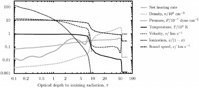
The net rate at which the gas gains energy from atomic processes (photoelectric heating minus radiative cooling; solid gray line) has two separate peaks in the front. The deeper peak occurs at $\tau\simeq 8$ and results in the heating of the gas from $100$ K to $9000$ K and its acceleration from $0.1\mathrm{\ km\ s^{-1}}$ to $3\mathrm{\ km\ s^{-1}}$, but leaves the gas still largely neutral ($x\simeq 0.01$). The shallower, broader peak occurs at $\tau\simeq 3$ and results in the complete ionization of the gas and its acceleration to $\simeq 10\mathrm{\ km\ s^{-1}}$, with very little change in temperature. The gas then passes through a sonic point at $\tau\simeq 1$, at which point $x\simeq 0.95$, and continues accelerating gradually up to $\simeq 30\mathrm{\ km\ s^{-1}}$ as it flows back past the star (not shown). Although the far downstream velocity of the ionized gas is supersonic, the front is still D-critical since there is no internal maximum in the sound speed. Instead, it is the divergence of the gas streamlines, as the geometry deviates from plane-parallel, that allow the gas to continue accelerating once it is fully ionized and isothermal.

The shock that precedes the ionization front is also visible, at depth of $\tau\simeq 50$. The shock is propagating into the neutral gas slightly faster than the ionization front velocity, so this part of the model is not exactly time-steady, but rather the column of shocked neutral material grows with time. This part of the structure is the least well-modeled in the simulation, since the physics of the photodissociation region is not treated adequately, but see Hosokawa & Inutsuka (2005b, a) for dynamical models that do treat this properly.

2.4 Photoablation flows

If the neutral density is similar in all directions from the ionizing star, then one would expect the radius to the ionization front to be also similar, which would lead to a global geometry for the front that is closed, or concave. Despite this, the opposite case is of great relevance to H  II region dynamics, in which the ionization front is convex; that is, it curves away from the ionizing star. This can arise, for example, if dense condensations exist in the neutral gas, which slow down the propagation of the ionization front, causing it to “wrap around” the obstacle. If this situation persists, then a steady flow of ionized gas will establish itself that accelerates away from the convex front. The density in this ionized photoablation flow increases sharply towards its base, where it may greatly exceed the mean density in the H  II region. Models for such flows were originally developed in the context of the photoevaporation of small, self-gravitating globules (Dyson 1968; Kahn 1969) but have a much wider range of application. By adopting a cylindrical, rather than spherical geometry, similar models can be applied to cases where the ionization front wraps around a dense filament, as in the Bright Bar in the Orion Nebula, and they can even be extended to cases where the ionization front is flat, or slightly concave, as in the case of champagne flows (see section 3.2 below). In all cases, the structure of the ionized flow is similar, provided only that the gas streamlines diverge and that any pressure imposed at the downstream boundary is low compared with the thermal pressure of the ionized gas at the ionization front. In order for a steady-state approach to be valid, it is also necessary that the timescale for significant changes in the configuration of the neutral gas be long compared with the dynamic timescale of the ionized flow. This condition is easily satisfied in some cases, such as the Orion proplyds, but only approximately satisfied in others, such as the radiation-driven implosion of a neutral globule (Bertoldi 1989).

The simplest models proceed by patching together the solution for a plane-parallel D-critical ionization front (see previous sections) with an isothermal wind solution for the fully ionized flow. This is valid so long as the width of the ionization front is very small compared with its radius of curvature, $r_{\mathrm{c}}$, which is almost invariably the case. The gas leaves the ionization front at the sound speed but accelerates rapidly (see Fig. 6 of Henney 2003), so that the ionized density falls off more quickly than it would in a constant velocity wind, approximately mimicking an exponential profile. As the Mach number of the flow increases, the acceleration gradually lessens and a terminal velocity is reached when the isothermal approximation breaks down, which occurs when the expansion and heating timescales becoming comparable. For a spherical flow with $\lambda_{\mathrm{ad}}=0.01$, this occurs at velocity of $\simeq 40\mathrm{\ km\ s^{-1}}$ and a radius of $\simeq 10r_{\mathrm{c}}$.

Unless the ionization parameter is rather low, $\lambda_{\mathrm{ad}}$ will be small and the flows are recombination dominated, which means that the ionized flow has a high optical depth to ionizing radiation and is in approximate static ionization balance. The effective recombination thickness of the flow is $h_{\mathrm{eff}}=0.12r_{\mathrm{c}}$ for a spherical geometry or $h_{\mathrm{eff}}=0.3r_{\mathrm{c}}$ for a cylindrical geometry, so long as the curvature is positive (convex) and $r_{\mathrm{c}}\ll r_{\star}$, where $r_{\star}$ is the distance of the front from the ionizing star. For the case where $r_{\mathrm{c}}>r_{\star}$, one instead finds $h_{\mathrm{eff}}\simeq 0.2$–$0.7r_{\star}$ (see Fig. 7 of Henney et al. 2005a). In either case, the entire flow structure is uniquely determined by the incident ionizing flux and the curvature of the front. If $r_{\mathrm{c}}\mathrel{\hbox{\footnotesize\hbox to0.0pt{\hbox{\lower 3.0pt\hbox{$\sim$}}\hss}\raise 1.5pt\hbox{$<$}}}0.2r_{\star}$, then the photoevaporation flow is not capable of evacuating the region all the way back to the ionizing star, so the incident flux may be reduced by recombinations in the interior of the H  II region.

2.5 Other ingredients

Stellar Winds

High mass stars invariably drive fast ($\simeq 1000\mathrm{\ km\ s^{-1}}$) stellar winds (Lamers & Cassinelli 1999), Wind mass loss rates are still very uncertain due to the poorly understood effects of clumping on observational diagnostics (Fullerton et al. 2006), but are probably in the range $10^{-9}$–$10^{-7}M_{\odot}\mathrm{\ yr^{-1}}$ for main-sequence O stars. The effect of a stellar wind on the dynamics of an H  II region depends crucially on whether or not a hot bubble of shocked stellar wind can persist, which determines whether the shell of shocked H  II region gas is energy-driven or momentum-driven (see the chapter by Arthur chapter in this volume). In the energy-driven case, Capriotti & Kozminski (2001) show that the shell swept up by the stellar wind can dominate the expansion energy of the region at early evolutionary times and when the ambient density is $>10^{4}\mathrm{\ cm^{-3}}$ (see also Dyson 1977; Garcia-Segura & Franco 1996). The wind-blown shell is also capable of trapping the ionization front in some instances. In the momentum-driven case, the wind never dominates the global energetics of the region but can nevertheless have an important local influence on the internal dynamics. One example is the bowshocks found around proplyds in the inner Orion Nebula (García-Arredondo et al. 2001). Various mechanisms may prevent the formation of the hot shocked bubble that is required for the energy-driven case, including thermal conduction (e.g., Dorland & Montmerle 1987) or dynamical instabilities (Breitschwerdt & Kahn 1988) at the contact discontinuity, or mass-loading of the wind due to embedded photoablating clumps or proplyds (Dyson et al. 1995; García-Arredondo et al. 2002). All these can cause enhanced cooling in the shocked wind, leading to the loss of its thermal pressure. Specific instances of the importance of winds in the evolution of H  II regions are described in section 3 below.

Radiation pressure

The transfer of momentum between the radiation field and the gas can sometimes affect the dynamics of H  II regions. This arises in three different ways: first, through trapped resonance line radiation (mainly Lyman $\ualpha$); second, through the momentum of stellar photons transferred during the photoionization process; and, third, indirectly through collisional coupling with dust grains that are accelerated by the absorption of stellar radiation.

Although the diffusion of resonance line photons can in principle introduce non-local couplings between disparate parts of an H  II region, this is severely hampered by the presence of dust absorption (Hummer & Kunasz 1980), which allows a purely local approach to be used if the medium is homogeneous on scales $<0.1/\kappa_{\mathrm{d}}$, where $\kappa_{\mathrm{d}}$ is the dust absorption coefficient. By this means, Henney & Arthur (1998) showed that the resonance line radiation pressure is proportional to the gas pressure, making a contribution of only $\simeq 5\%$ for a standard dust-gas-ratio.

The radiative acceleration due to absorption of ionizing photons of mean energy $\langle h\nu\rangle$ is $g_{\mathrm{rad}}\simeq(\langle h\nu\rangle/c)(f/\rho h_{\mathrm{abs}})$, where $h_{\mathrm{abs}}$ is the thickness over which the photons are absorbed. The acceleration due to pressure gradients in a photoablation flow (section 2.4) is $g_{\mathrm{flow}}\simeq a^{2}/h_{\mathrm{eff}}$. Comparing the two, and putting $h_{\mathrm{abs}}=h_{\mathrm{eff}}$, one finds $g_{\mathrm{rad}}/g_{\mathrm{flow}}\simeq\varUpsilon\langle h\nu\rangle/(2kT)\sim 10\varUpsilon$, so that the pressure of the ionizing radiation is of only secondary importance unless the ionization parameter is higher than is typically found in H  II regions. Assuming that the gas and grains are effectively coupled, one finds a similar result for the absorption of radiation by dust, although this can become more important for cooler stars, where the relative luminosity at non-ionizing wavelengths is higher. Radiation pressure on dust can also be important in the inner parts of H  II regions due to the increased flux close to the ionizing source, where it may be responsible for central cavities in some cases (Mathews 1967; Inoue 2002).

Magnetic fields

The magnetic field makes a significant, perhaps dominant, contribution to the pressure both in molecular clouds and in the diffuse ISM. H  II regions are generally over-pressured with respect to their undisturbed surroundings, but are within a factor of two of pressure equilibrium with the shocked neutral gas that surrounds them. The dynamic importance of magnetic fields inside the H  II region depends sensitively on how the field strength, $B$, responds to compression in the shock and rarefaction at the ionization front. This can be approximately characterized by an effective adiabatic index, $\gamma_{\mathrm{m}}$, such that $B^{2}\propto\rho^{\gamma_{\mathrm{m}}}$. Possible values of this index are bounded by $\gamma_{\mathrm{m}}=0$ for compression/rarefaction parallel to the field lines of an ordered field and $\gamma_{\mathrm{m}}=2$ for compression/rarefaction perpendicular to the field, whereas $\gamma_{\mathrm{m}}\mathrel{\hbox{\footnotesize\hbox to0.0pt{\hbox{\lower 3.0pt\hbox{$\sim$}}\hss}\raise 1.5pt\hbox{$<$}}}1$ seems to be indicated by observations. The order-of-magnitude increase in sound speed between the ionized and neutral gas means that the plasma $\beta$-parameter (ratio of gas pressure to magnetic pressure) will be between 5 times (if $\gamma_{\mathrm{m}}=0$) and 2000 times (if $\gamma_{\mathrm{m}}=2$) higher in the H  II region than in the undisturbed neutral gas, assuming the H  II region to be five times overpressured. Thus, it is plausible that the magnetic field should play a much lesser role in the ionized gas than in the neutral gas. Nevertheless, the magnetic fields can still have dramatic effects on H  II region dynamics, particularly for the ionization front, and magnetohydrodynamic models of these are presented in detail in the chapter by Williams chapter in this volume.

Instabilities

The dynamics of the photoionized gas will also be influenced by many different kinds of instabilities (see Williams 2003 for an overview), which may contribute to the detailed structure observed in H  II regions. Different modes of instability at the ionization front are found, depending on whether the shell of shocked neutral gas outside it is thick (Williams 2002) or thin (Giuliani 1979; Garcia-Segura & Franco 1996). Recombinations in the fully ionized gas are found to damp the instabilities in some (Axford 1964; Mizuta et al. 2005) but not all (Williams 2002) cases. The interaction between streams of gas inside the H  II region, such as stellar winds or photoablation flows, provides opportunities for further instabilities (e.g., Rayleigh-Taylor, Kelvin-Helmholtz) and these may interact with ionization front instabilities in complicated ways. An example is shown in the simulations of Arthur & Hoare (2005), where the fragmention of a wind-driven shell triggers shadowing instabilities of the type discussed by Williams (1999).

3 H  II region evolution

While the classical scenario for the expansion of an ionized Strömgren sphere in a constant density medium has clear didactic value, it not necessarily relevant to the evolution of real H  II regions. Massive stars form in dense and highly inhomogeneous molecular clouds and begin to emit ionizing photons while they are still accreting mass, possibly via a disk (see the chapter by Franco & Hoare chapter in this volume for an overview of high-mass star formation). Various mechanisms may act to prolong the duration of the early phases of evolution, either by physical confinement or by providing a reservoir of neutral gas. Eventually the H  II region may break out from the molecular cloud and become optically visible, but its evolution will still be strongly affected by the strong density gradients in its environment. Since high-mass star formation is strongly clustered, extended H  II regions will tend to be excited by multiple OB stars. As the region’s age begins to exceed the main-sequence lifetime of the highest mass stars, then the powerful winds from evolved stars and subsequent supernova explosions will have a dramatic effect on the dynamics.

3.1 Early phases: hypercompact and ultracompact regions

The smallest observed H  II regions are of size $\sim 10^{-3}$ parsec, and are classified as hypercompact regions (Carral et al. 1997; Sewilo et al. 2004). At these small sizes, the escape velocity at the ionization front is larger than the ionized sound speed, and so gravitational effects are important. If the central star is still accreting via a spherical Bondi-Hoyle flow, then the accretion velocity just outside the ionization front exceeds the R-critical velocity of $2c_{\mathrm{i}}$, so the gas suffers only a mild deceleration in the front and continues its accretion onto the star (Keto 2002). During this phase, the ionization front does not expand dynamically, but can only increase its radius if the ionizing luminosity of the central star increases (Keto 2003). This phase is therefore rather long-lived, with a duration given by the timescale for the nascent star to grow by accretion, of order $10^{5}$ years.

H  II regions with sizes $\sim 0.01$–$0.1$ parsec and densities $>10^{5}\mathrm{\ cm^{-3}}$ are classified as ultracompact and these are much more numerous and well-studied than the hypercompact regions (e.g., Wood & Churchwell 1989; Kurtz et al. 1994; de Pree et al. 2005). They show a diverse range of morphologies, such as cometary, shell-like, bipolar, or irregular, although roughly half are spherical or unresolved. The high number of observed ultracompact H  II regions in the galaxy has been taken to imply a lifetime for this phase of $\simeq 10^{6}$ years (Wood & Churchwell 1989), although it should be noted that other estimates are as short as $5\times 10^{4}$ years (Comeron & Torra 1996). A remarkable diversity of dynamical models have been proposed in order to explain this lifetime, which is longer than the time for a classical Strömgren sphere to expand past $0.1$ parsec. In some models, the ionized gas is physically confined to ultracompact sizes, either by the ram pressure of the ambient medium as the star moves through the molecular gas (van Buren et al. 1990), or by an accretion flow onto the star (Keto 2002; González-Avilés et al. 2005), or merely by the high static pressure (thermal plus magnetic plus turbulent) of the molecular cloud core (de Pree et al. 1995; Garcia-Segura & Franco 1996). Other models allow the ionized gas to expand freely but provide a reservoir of neutral gas, the photoablation of which sustains the brightness of the ultracompact core: either an accretion disk around the high-mass star (Hollenbach et al. 1994; Yorke & Welz 1996; Richling & Yorke 1997; Lugo et al. 2004), or dense neutral clumps (Dyson et al. 1995; Lizano et al. 1996; Redman et al. 1996). In many instances, ultracompact H  II regions are seen to be embedded in larger-scale, more diffuse emission (Kurtz et al. 1999), which would tend to favor the second class of models if the extended emission were physically connected with the ultracompact region. However, it is entirely possible that each of these models is applicable to some subclass of ultracompact regions.

3.2 Later phases: compact and extended regions

At least some ultracompact H  II regions eventually expand to larger sizes, forming the class of compact H  II regions (Mezger et al. 1967), with sizes $0.1$–$0.5$ parsec and densities $\simeq 10^{4}\mathrm{\ cm^{-3}}$. Most compact regions are embedded inside extended H  II regions, which are typically several parsecs in size, with densities $\simeq 100\mathrm{\ cm^{-3}}$. The distribution of morphological types is similar to that for ultracompact regions (Hunter 1992; Fich 1993), although most modeling effort has gone into explaining the cometary shaped regions. These are similar in appearance to many optically visible H  II regions, which are classified as blister-type (Israel 1978), and of which the best-known example is the Orion Nebula (O’Dell 2001). The low extinction to these optical regions proves that they must be on the near side of any accompanying molecular gas, and they generally show blueshifted velocities of order the ionized sound speed in optical emission lines, indicative of flow away from the molecular cloud (Zuckerman 1973). A broad class of models, commonly referred to as champagne flows, has been proposed to account for these objects. These models share the property that strong density gradients in the neutral/molecular gas allow the ionization front to break out in some directions, leading to a flow of high-pressure ionized gas in the same direction. The original model of Tenorio-Tagle (1979) considered the one-dimensional propagation of an ionization front inside a dense cloud with a sharp edge. Once the ionization front reaches the edge of the cloud, it rapidly propagates through the much rarer intercloud medium and is followed by a strong shock that is driven by the higher pressure ionized cloud material. A rarefaction wave simultaneously travels back into the ionized cloud, initiating the champagne flow that accelerates the ionized gas up to several times the ionized sound speed as it flows away from the cloud. Following studies extended this work to two dimensions (see references in Yorke 1986, section 3.3) and considered the effects of disk-shaped clouds and more gradual cloud boundaries.

Figure 2: Simulations of quasi-steady champagne flows, produced by the ionization of the interface of a dense molecular cloud (adapted from Henney et al. 2005a). Three different models (top to bottom) are shown with different lateral density profiles in the neutral gas. The left panels shows the ionized density, while the right panels show the total pressure with superimposed streamlines, the darkness of which indicates the gas velocity. The position of the ionizing star is shown by a black circle in each case.

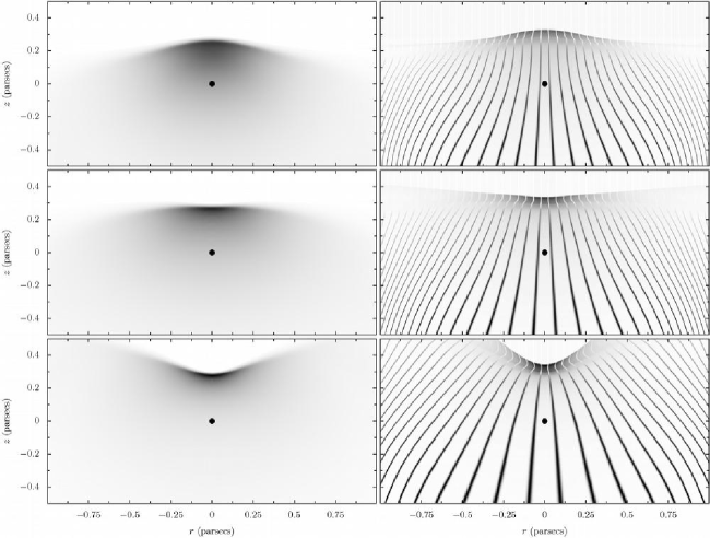
Early work on the dynamics of champagne flows considered scenarios that were intrinsically non-steady. However, it is also possible to construct quasi-stationary champagne flow models (Henney et al. 2005a) in which the structure of the ionized flow remains constant over several times its dynamical timescale. These models are valid so long as the density of the neutral gas that confines the ionization front on one side is high enough that the ionization front moves slowly and encounters constant upstream conditions during the evolution. It can be shown that in the steady-state limit a divergence of the ionized flow is necessary in order to produce significant acceleration. This is beacuse in a strictly plane-parallel geometry, and in the absence of body forces, the acceleration is proportional to the gradient of the sound speed, which is almost zero in the isothermal ionized gas. Examples of such flows with different degrees of divergence are shown in Fig. 2. The degree of divergence is controlled by the neutral density profile in the lateral direction (perpendicular to the sharp density gradient at the surface of the cloud). When this density profile is constant, as in the upper panels of Fig. 2, the ionization front is concave (negative curvature), leading to weak divergence of the flow and slow acceleration. For a steep lateral density profile, as in the lower panels of Fig. 2, the ionization front becomes convex (positive curvature), giving a strong, almost spherical, divergence to the flow, which now accelerates much more strongly. This configuration is similar to that seen in globule flows. Approximate analytic calculations suggest that the ionization front should be flat when the lateral density profile is proportional to $1/(1+r^{2})$, in which the distance, $r$, from the symmetry axis has been scaled by the axial offset between the star and the ionization front. Numerical simulations confirm that this is indeed the case, as shown in the central panels of Fig. 2.

Ginwidth=0.47

Figure 3: Simulations of the interaction of a champagne flow with a stellar wind (from Arthur & Hoare 2005). Grayscale shows log of ionized density and arrows show gas velocity on two different scales: the longest white arrow represents $30\mathrm{\ km\ s^{-1}}$ while the longest black arrow represents $2000\mathrm{\ km\ s^{-1}}$. The left panel shows a model with a weak wind (mass loss rate of $10^{-7}M_{\odot}\mathrm{\ yr^{-1}}$) and the right panel shows a model with a strong wind ($10^{-6}M_{\odot}\mathrm{\ yr^{-1}}$). Both models have a wind velocity of $2000\mathrm{\ km\ s^{-1}}$ and an ionizing photon luminosity of $2.2\times 10^{48}\mathrm{\ s}^{-1}$.

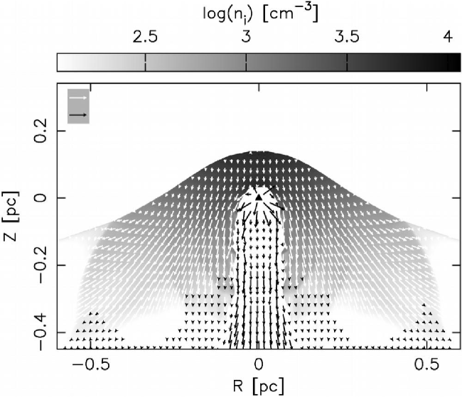
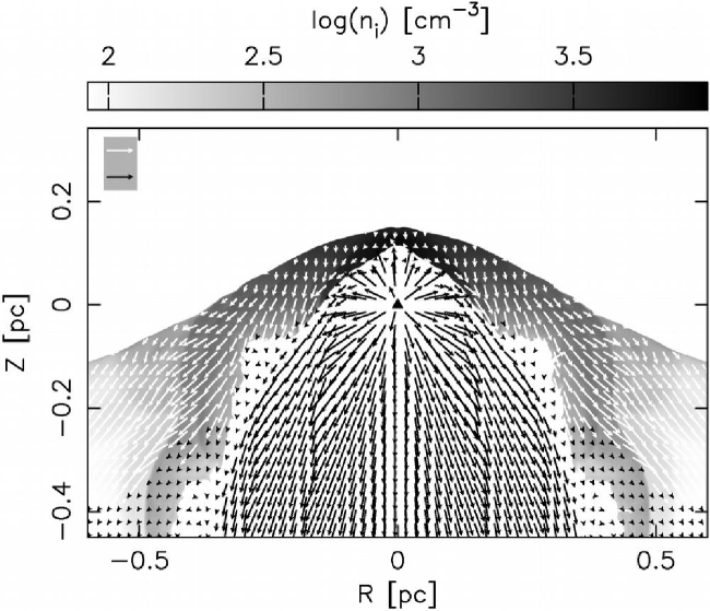
The stellar wind from the ionizing star may also be expected to have an effect on the dynamics of the champagne flow and this was first modelled by Comeron (1997). An alternative explanation for the cometary shapes shown by many regions is the bowshock model van Buren et al. (1990) previously discussed in the context of ultracompact regions. In this model, the ionizing star moves supersonically through the molecular gas and the ionization front is trapped in the dense shocked shell formed by the interaction between the stellar wind and the ambient gas. An extension of this scenario was studied by Franco et al. (2005), in which the ionizing star moves in and out of a high density molecular cloud core. An exhaustive study of the interplay between champagne flows, stellar winds, and stellar motion was carried out by Arthur & Hoare (2005), who found a great variation in the resultant morphology, depending on the strength of the stellar wind. All the Arthur & Hoare models have concave ionization fronts, as in the top row of Fig. 2. If the stellar wind is weak, as in the first panel of Fig. 3, then the champagne flow is hardly affected, except in a narrow region around the axis, where it forms a weak bowshock around the stellar wind. A stronger stellar wind, as in the second panel of Fig. 3 has a much more dramatic effect. The point of pressure balance along the axis between the stellar wind and the H  II region gas is pushed closer to the ionization front than where the sonic point would have been in the champagne flow. As a result, there is no champagne flow on the axis, although away from the axis a transonic champagne flow does develop, which then shocks against the stellar wind. The large obstacle provided by the wind means that the champagne flow acceleration is predominantly parallel to the ionization front in this case. The inclusion of a stellar velocity in the direction of increasing gradient produces only small changes in the results unless the stellar velocity is higher than the ionized sound speed. Such models always show a greater resemblance to champagne flow models than to classical bowshock models unless the density gradient in the neutral cloud is very shallow. Either cometary or shell-like morphologies can be produced, depending on the steepness of the neutral density distribution.

Another class of models considers the radial expansion of an H  II region in a spherical cloud with a density distribution steeper than $r^{-3/2}$ (Franco et al. 1990; Shu et al. 2002; Lizano et al. 2003), in which no static equilibrium solution exists for the position of the ionization front. When the star turns on, an R-type ionization front quickly propagates to large radii, and the ionized gas adopts a configuration in which a roughly uniform density core, bounded by a shock, expands slightly faster than the ionized sound speed. Such a region is doomed to rapidly decline in brightness after a few sound crossing times. Confusingly, these entirely density-bounded models are also referred to as champagne flows, although they are significantly different from the models considered in the previous paragraph. A classical champagne flow is ionization-bounded on at least one side and will maintain a high brightness indefinitely, as long as sufficient neutral gas exists to confine the ionization front close to the ionizing star on that side.

At even larger scales, any expansion of the H  II region will stop when it comes into pressure balance with the local interstellar medium. The mean pressure in spiral arms at radius of solar circle is $\simeq 5\times 10^{4}~{}\mathrm{K\ cm^{-3}}$, which is 90% non-thermal (Cox 2005). This would balance that of the ionized gas when its density has fallen to a few $\mathrm{cm^{-3}}$. The equivalent Strömgren radius is $\simeq 30$ parsec for a typical O star, but would be would be larger for regions ionized by a cluster of stars, in which case vertical density gradients in the disk may become important. However, the time required for an H  II region to expand to such sizes is comparable with the evolutionary timescales for high-mass stars, so that the powerful winds from the later stages of stellar evolution and the expansion of supernova remnants will have a profound effect on the dynamics of the region. Similar considerations apply to H  II regions seen in external galaxies (Shields 1990), although the largest H  II regions ($>500$ parsec) show highly supersonic velocities (e.g., Terlevich & Melnick 1981; Gallagher & Hunter 1983; Relaño et al. 2005), which correlate with the luminosity of the region and may be indicative of virial equilibrium of the ionized gas in the gravitational potential of the star cluster.

3.3 Clumps and turbulence

One shortcoming of the models mentioned in the previous section is that they consider only smooth density distributions for the neutral gas into which the H  II region propagates. In reality, this is unlikely to be the case, since the molecular clouds in which high-mass stars form are known to be highly structured, which is probably the result of supersonic turbulence (Elmegreen & Scalo 2004). Dynamic models that attempt to take into account the clumpy nature of the neutral gas were first proposed by John Dyson and collaborators (Dyson et al. 1995; Williams et al. 1996; Redman et al. 1996, 1998) in order to explain the morphology and lifetimes of ultracompact H  II regions. In these models dense neutral clumps are assumed to be distributed throughout the ionized volume and to act as mass-loading sites for a stellar wind from the ionizing star. The models are agnostic with respect to the physics of the mass injection process, which is not modeled directly, but which may be ablation by photoionization or hydrodynamic processes. Instead, the flow is treated statistically under the assumption of prompt and complete mixing of the ablated gas with the stellar wind. Similar models have also been presented that treat the ablation process in more detail and explicitly allow for the finite lifetime of the clumps (Lizano et al. 1996; Arthur & Lizano 1997). Both sets of models result in a shell-like morphology for the H  II region (if the clumps are distributed uniformly), bounded by a recombination front through which the ionized wind flows.

Figure 4: Three-dimensional simulation of the photoevaporation of a clumpy self-gravitating globule (adapted from Kessel-Deynet & Burkert 2003). Left: Phase of maximum compression, $1.6\times 10^{5}$ years. Center: Equilibrium cometary phase, $2.8\times 10^{5}$ years. Right: Fragmentaion phase, $4.2\times 10^{5}$ years. The grayscale measures the absolute value of the difference between the column density of the ionized and neutral gas (white corresponds to the ionization front). Box size is 0.85 parsec in the left panel and 1.8 parsec in the other panels.

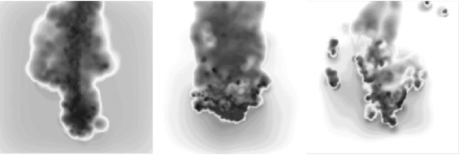
A more detailed treatment of the interaction of ionizing photons with a clumpy medium is possible only with three-dimensional numerical simulations. The first such simulation to be carried out studied the response of a static equilibrium self-gravitating spherical globule to an external ionizing flux (Kessel-Deynet & Burkert 2003). The density distribution of the initial globule (of mass 40 $M_{\odot}$ and radius $1$ parsec, on the margin of Jeans instability) is perturbed by Gaussian fluctuations of amplitude $\simeq 50\%$. It is found that the turbulence generated behind the shock driven into the globule by the ionization front is sufficient to prevent gravitational collapse of the globule at its point of maximum compression, despite collapse having occurred at this point in a companion simulation of a globule without density perturbations. After $\simeq 5\times 10^{5}$ years, the neutral gas that has survived photoablation has broken up into smaller sub-globules (Fig. 4). Similiar simulations have also been carried out of the photoevaporation of much smaller, non-self-gravitating, clumpy globules (González et al. 2005). In this case, although some fragmentation of the globule occurs, the fragments remain physically attached to one another until the globule is completely evaporated.

Figure 5: Dynamical evolution of an H 

II

region in a turbulent molecular cloud, adapted from Mellema et al. (2005). For each of two evolutionary times, 100,000 and 300,000 years, five $yz$ slices through the $(4~{}\mathrm{parsec})^{3}$ computational box are shown, with offsets from the ionizing star as shown on the bottom axis. Density is shown on a negative logarithmic scale between 10 (white) and $10^{5}~{}\mathrm{cm}^{−3}$ (black). Temperature is shown on a positive linear scale between 0 (black) and $10^{4}$ K (white).

Simulations of hydrodynamical and magnetohydrodynamical turbulence in molecular clouds (e.g., Mac Low 1999; Vázquez-Semadeni et al. 2005) have now reached a level of refinement that makes them suitable to use as initial conditions for the evolution of H  II regions. Li et al. (2004) carried out a preliminary investigation of this problem by studying only the initial R-type propagation of the ionization front, before the dynamics of the ionized gas becomes important. This approach was extended by Mellema et al. (2005), who carried out a full radiation-hydrodynamic simulation of the evolution of an H  II region in a turbulent medium, following the birth of an $\simeq 25~{}M_{\odot}$ star inside the densest molecular clump ($\simeq 10^{6}~{}\mathrm{cm}^{-3}$) that formed in the Vázquez-Semadeni et al. (2005) turbulence simulation.

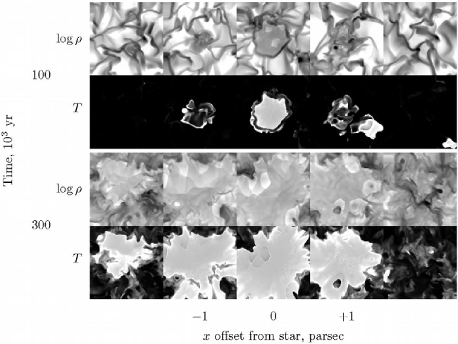
The results of this simulation are shown in Fig. 5 for two evolutionary times. At the earlier time, the H  II region is mainly confined to a compact core of radius $\simeq 1$ parsec, although the ionization front has already broken out to the boundary of the grid through a corridor of low-density neutral gas in one direction, as can be seen in the lower-right corner of the rightmost temperature image. The density variations in the ionized gas are rather mild compared with those in the neutral gas and are of a different nature. Instead of dense sheets and filaments, one finds an almost constant density gas filling roughly half of the ionized region, with the remainder occupied by low-density cavities carved out by transonic photoablation flows, as described in section 2.4 (see also Williams et al. 2001; Henney 2003). This structure of the ionized gas can be better appreciated at the later evolutionary time, where multiple photoablation flows are seen, streaming off dense neutral condensations. The highest ionized densities are found at the ionization fronts of these flows and their mutual collisions produce many weak shocks, which generate density structure in the interior of the H  II region. Some of these structures become compressed sufficiently to significantly absorb the ionizing photons, causing the ionized gas beyond them to temporarily recombine. Regions where this has occured can be seen as intermediate-temperature gas in the bottom row of Fig. 5. The photoablation flows help maintain a high velocity dispersion of the ionized gas, which remains roughly equal to the ionized sound speed during the entire evolution, even though the net radial expansion velocity falls to much lower values (Mellema et al. 2005, Fig. 4). This mechanism is similar to that proposed by Dyson (1968) to explain the velocity dispersion observed in the Orion Nebula.

Figure 6: Fake emission line images from the simulation shown in Fig. 5 at an evolutionary time of 400,000 years. Top row: [$\mathrm{N\,\scriptstyle II}$] 6584 Å. Bottom row: [$\mathrm{O\,\scriptstyle III}$] 5007 Å. Views along the $x$, $y$, and $z$ axes are shown from left to right, respectively.

Figure 7: The Lagoon Nebula (M8). Combination of red and infrared continuum images from the Second Epoch Sky Survey of the UK Schmidt Telescope, operated by the Anglo-Australian Observatory, digitized by the Space Telescope Science Institute. A highly non-linear grayscale mapping has been used to show both bright and faint structures at the same time. The field of view is $\simeq 27\times 21$ parsec, assuming a distance of 1500 parsec.

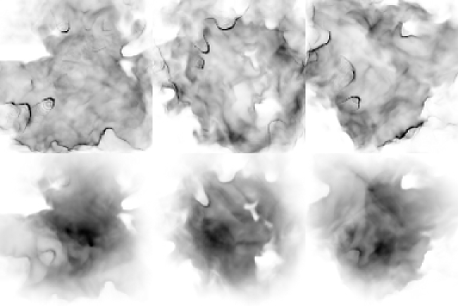
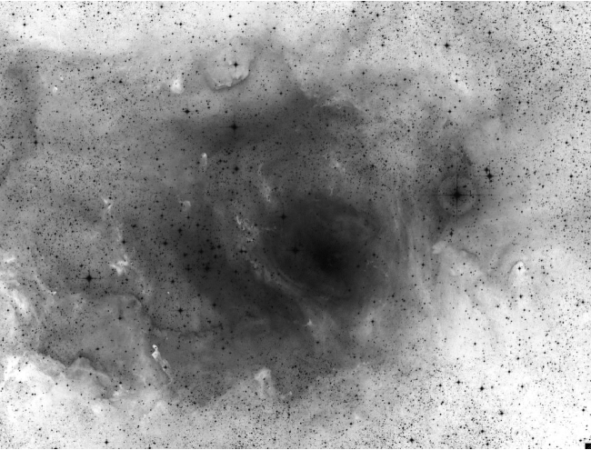
The predicted appearance of these simulations in optical emission lines is shown in Fig. 6. The [$\mathrm{N\,\scriptstyle II}$] line traces the low-ionization gas close to the ionization front, and these images are dominated by the bright rims of photoablation flows, while the [$\mathrm{O\,\scriptstyle III}$] line traces the higher ionization gas in the interior of the nebula, which shows a more diffuse aspect in the images. The predicted emission line structure is very similar to that observed in real nebulae, such as the Lagoon Nebula shown in Fig. 7. The broad-band filters used in that image include optical emission lines of both low and high ionization, so it should be compared with the superposition of the [$\mathrm{N\,\scriptstyle II}$] and [$\mathrm{O\,\scriptstyle III}$] images (see Fig. 1 of Dufour 1994 for pure emission line images of the inner regions of this nebula). As in the simulations, one sees sharply bounded bright arcs and dark extinction features in the low-ionization periphery of the nebula, together with more diffuse emission in the higher ionization core. It should be noted that the Lagoon Nebula is several times larger than the simulation and is ionized by several massive stars, but a similar morphology is seen in more compact nebulae, such as M16, M20, and M42.

Such sculpted structures at the boundary of the nebula can also be produced via instabilities, even if the ambient neutral gas is initially smoothly distributed (e.g., Garcia-Segura & Franco 1996). A clear example of this is seen in Fig. 3 of Williams (2003), where large-scale density gradients lead to a thin-shell instability and the formation of multiple photoablation flows from the now clumpy shocked neutral layer. Whether ionization front instabilities or pre-exisiting structures in the neutral gas are more important in a given region is still an open question. However, the density contrasts found in molecular clouds on parsec scales are much more extreme than those seen in H  II regions, due to the highly supersonic nature of the turbulence and the effects of self-gravity. Thus, it seems likely that the structure of the neutral gas is dominant in shaping H  II regions at these scales. At smaller scales, the turbulent velocity dispersion, and hence the density contrast, is much reduced, so that ionization front instabilities may play a more important role, although these tend to saturate at amplitudes of order the recombination length (Williams 2002), which is approximately ten times the ionization front thickness, or $\simeq n^{-1}$ parsec, where $n$ is measured in $\mathrm{cm^{-3}}$.

Summary

H  II regions, particularly the extended, optically visible variety have the reputation of being “messy” objects, ill-suited to the austere theoretical prejudice of perfect symmetry. However, as I have tried to illustrate in this review, even their messiest aspects are beginning to fall under the purview of dynamic modelling. We are still some way from a totally satisfactory model of any particular object, let alone H  II regions as a class, but a large amount of progress has been made.

References

- Arthur & Hoare (2005) Arthur, S. J. & Hoare, M. G. 2005, arXiv:astro-ph/0511035
- Arthur et al. (2004) Arthur, S. J., Kurtz, S. E., Franco, J., & Albarrán, M. Y. 2004, ApJ, 608, 282
- Arthur & Lizano (1997) Arthur, S. J. & Lizano, S. 1997, ApJ, 484, 810
- Axford (1964) Axford, W. I. 1964, ApJ, 140, 112
- Bertoldi (1989) Bertoldi, F. 1989, ApJ, 346, 735
- Breitschwerdt & Kahn (1988) Breitschwerdt, D. & Kahn, F. D. 1988, MNRAS, 235, 1011
- Capriotti & Kozminski (2001) Capriotti, E. R. & Kozminski, J. F. 2001, PASP, 113, 677
- Carral et al. (1997) Carral, P., Kurtz, S. E., Rodriguez, L. F., de Pree, C., & Hofner, P. 1997, ApJ, 486, L103+
- Comeron (1997) Comeron, F. 1997, A&A, 326, 1195
- Comeron & Torra (1996) Comeron, F. & Torra, J. 1996, A&A, 314, 776
- Cox (2005) Cox, D. P. 2005, ARA&A, 43, 337
- de Pree et al. (1995) de Pree, C. G., Rodriguez, L. F., & Goss, W. M. 1995, Revista Mexicana de Astronomia y Astrofisica, 31, 39
- de Pree et al. (2005) de Pree, C. G., Wilner, D. J., Deblasio, J., Mercer, A. J., & Davis, L. E. 2005, ApJ, 624, L101
- Dorland & Montmerle (1987) Dorland, H. & Montmerle, T. 1987, A&A, 177, 243
- Dufour (1994) Dufour, R. J. 1994, Revista Mexicana de Astronomia y Astrofisica, 29, 88
- Dyson (1968) Dyson, J. E. 1968, Ap&SS, 1, 388
- Dyson (1977) —. 1977, A&A, 59, 161
- Dyson & Williams (1997) Dyson, J. E. & Williams, D. A. 1997, The physics of the interstellar medium (Bristol: Institute of Physics Publishing)
- Dyson et al. (1995) Dyson, J. E., Williams, R. J. R., & Redman, M. P. 1995, MNRAS, 277, 700
- Elmegreen & Scalo (2004) Elmegreen, B. G. & Scalo, J. 2004, ARA&A, 42, 211
- Ercolano et al. (2005) Ercolano, B., Barlow, M. J., & Storey, P. J. 2005, MNRAS, 362, 1038
- Fich (1993) Fich, M. 1993, ApJS, 86, 475
- Franco et al. (2005) Franco, J., Garcia-Segura, G., & Kurtz, S. 2005, arXiv:astro-ph/0508467
- Franco et al. (1990) Franco, J., Tenorio-Tagle, G., & Bodenheimer, P. 1990, ApJ, 349, 126
- Fullerton et al. (2006) Fullerton, A. W., Massa, D. L., & Prinja, R. K. 2006, ApJ, 637, 1025
- Gail & Sedlmayr (1979a) Gail, H.-P. & Sedlmayr, E. 1979a, A&A, 77, 165
- Gail & Sedlmayr (1979b) —. 1979b, A&A, 76, 158
- Gallagher & Hunter (1983) Gallagher, J. S. & Hunter, D. A. 1983, ApJ, 274, 141
- García-Arredondo et al. (2002) García-Arredondo, F., Arthur, S. J., & Henney, W. J. 2002, Revista Mexicana de Astronomia y Astrofisica, 38, 51
- García-Arredondo et al. (2001) García-Arredondo, F., Henney, W. J., & Arthur, S. J. 2001, ApJ, 561, 830
- Garcia-Segura & Franco (1996) Garcia-Segura, G. & Franco, J. 1996, ApJ, 469, 171
- Giuliani (1979) Giuliani, J. L. 1979, ApJ, 233, 280
- González et al. (2005) González, R. F., Raga, A. C., & Steffen, W. 2005, Revista Mexicana de Astronomia y Astrofisica, 41, 443
- González-Avilés et al. (2005) González-Avilés, M., Lizano, S., & Raga, A. C. 2005, ApJ, 621, 359
- Henney (2001) Henney, W. J. 2001, in The Seventh Texas-Mexico Conference on Astrophysics: Flows, Blows and Glows (Eds. William H. Lee and Silvia Torres-Peimbert) Revista Mexicana de Astronomía y Astrofísica (Serie de Conferencias) Vol. 10, 57–60
- Henney (2003) Henney, W. J. 2003, in Winds, bubbles, and explosions: a conference to honor John Dyson (Eds. S. J. Arthur and W. J. Henney) Revista Mexicana de Astronomia y Astrofisica Conference Series Vol. 15, 175–180
- Henney & Arthur (1998) Henney, W. J. & Arthur, S. J. 1998, AJ, 116, 322
- Henney et al. (2005a) Henney, W. J., Arthur, S. J., & García-Díaz, M. T. 2005a, ApJ, 627, 813
- Henney et al. (2005b) Henney, W. J., Arthur, S. J., Williams, R. J. R., & Ferland, G. J. 2005b, ApJ, 621, 328
- Hollenbach et al. (1994) Hollenbach, D., Johnstone, D., Lizano, S., & Shu, F. 1994, ApJ, 428, 654
- Hosokawa & Inutsuka (2005a) Hosokawa, T. & Inutsuka, S.-i. 2005a, arXiv:astro-ph/0511165
- Hosokawa & Inutsuka (2005b) —. 2005b, ApJ, 623, 917
- Hummer & Kunasz (1980) Hummer, D. G. & Kunasz, P. B. 1980, ApJ, 236, 609
- Hunter (1992) Hunter, D. A. 1992, ApJS, 79, 469
- Inoue (2002) Inoue, A. K. 2002, ApJ, 570, 688
- Israel (1978) Israel, F. P. 1978, A&A, 70, 769
- Kahn (1954) Kahn, F. D. 1954, Bull. Astron. Inst. Netherlands, 12, 187
- Kahn (1969) Kahn, F. D. 1969, Physica, 41, 172
- Kessel-Deynet & Burkert (2003) Kessel-Deynet, O. & Burkert, A. 2003, MNRAS, 338, 545
- Keto (2002) Keto, E. 2002, ApJ, 580, 980
- Keto (2003) —. 2003, ApJ, 599, 1196
- Kurtz et al. (1994) Kurtz, S., Churchwell, E., & Wood, D. O. S. 1994, ApJS, 91, 659
- Kurtz et al. (1999) Kurtz, S. E., Watson, A. M., Hofner, P., & Otte, B. 1999, ApJ, 514, 232
- López-Martín et al. (2001) López-Martín, L., Raga, A. C., Mellema, G., Henney, W. J., & Cantó, J. 2001, ApJ, 548, 288
- Lamers & Cassinelli (1999) Lamers, H. J. G. L. M. & Cassinelli, J. P. 1999, Introduction to Stellar Winds (UK: Cambridge University Press)
- Li et al. (2004) Li, Y., Mac Low, M.-M., & Abel, T. 2004, ApJ, 610, 339
- Lizano et al. (1996) Lizano, S., Canto, J., Garay, G., & Hollenbach, D. 1996, ApJ, 468, 739
- Lizano et al. (2003) Lizano, S., Galli, D., Shu, F., & Cantó, J. 2003, in Winds, bubbles, and explosions: a conference to honor John Dyson (Eds. S. J. Arthur and W. J. Henney) Revista Mexicana de Astronomia y Astrofisica Conference Series Vol. 15, 166–171
- Lugo et al. (2004) Lugo, J., Lizano, S., & Garay, G. 2004, ApJ, 614, 807
- Mac Low (1999) Mac Low, M.-M. 1999, ApJ, 524, 169
- Mathews (1967) Mathews, W. G. 1967, ApJ, 147, 965
- Mellema et al. (2005) Mellema, G., Arthur, S. J., Henney, W. J., Iliev, I. T., & Shapiro, P. R. 2005, arXiv:astro-ph/0512554
- Mezger et al. (1967) Mezger, P. G., Altenhoff, W., Schraml, J., Burke, B. F., Reifenstein, E. C., & Wilson, T. L. 1967, ApJ, 150, L157
- Mihalas (1978) Mihalas, D. 1978, Stellar atmospheres (San Francisco: W. H. Freeman and Co.)
- Mizuta et al. (2005) Mizuta, A., Kane, J. O., Pound, M. W., Remington, B. A., Ryutov, D. D., & Takabe, H. 2005, ApJ, 621, 803
- O’Dell (2001) O’Dell, C. R. 2001, ARA&A, 39, 99
- O’Dell et al. (2005) O’Dell, C. R., Henney, W. J., & Ferland, G. J. 2005, AJ, 130, 172
- Osterbrock & Ferland (2006) Osterbrock, D. E. & Ferland, G. J. 2006, Astrophysics of gaseous nebulae and active galactic nuclei (Sausalito, CA: University Science Books)
- Redman et al. (1996) Redman, M. P., Williams, R. J. R., & Dyson, J. E. 1996, MNRAS, 280, 661
- Redman et al. (1998) —. 1998, MNRAS, 298, 33
- Relaño et al. (2005) Relaño, M., Beckman, J. E., Zurita, A., Rozas, M., & Giammanco, C. 2005, A&A, 431, 235
- Richling & Yorke (1997) Richling, S. & Yorke, H. W. 1997, A&A, 327, 317
- Sewilo et al. (2004) Sewilo, M., Churchwell, E., Kurtz, S., Goss, W. M., & Hofner, P. 2004, ApJ, 605, 285
- Shapiro et al. (2005) Shapiro, P. R., Iliev, I. T., Alvarez, M. A., & Scannapieco, E. 2005, arXiv:astro-ph/0507677
- Shields (1990) Shields, G. A. 1990, ARA&A, 28, 525
- Shu (1992) Shu, F. H. 1992, Physics of Astrophysics, Vol. II (University Science Books)
- Shu et al. (2002) Shu, F. H., Lizano, S., Galli, D., Cantó, J., & Laughlin, G. 2002, ApJ, 580, 969
- Tenorio-Tagle (1979) Tenorio-Tagle, G. 1979, A&A, 71, 59
- Terlevich & Melnick (1981) Terlevich, R. & Melnick, J. 1981, MNRAS, 195, 839
- van Buren et al. (1990) van Buren, D., Mac Low, M.-M., Wood, D. O. S., & Churchwell, E. 1990, ApJ, 353, 570
- Vázquez-Semadeni et al. (2005) Vázquez-Semadeni, E., Kim, J., Shadmehri, M., & Ballesteros-Paredes, J. 2005, ApJ, 618, 344
- Williams (1999) Williams, R. J. R. 1999, MNRAS, 310, 789
- Williams (2002) —. 2002, MNRAS, 331, 693
- Williams (2003) Williams, R. J. R. 2003, in Winds, bubbles, and explosions: a conference to honor John Dyson (Eds. S. J. Arthur and W. J. Henney) Revista Mexicana de Astronomia y Astrofisica Conference Series Vol. 15, 184–189
- Williams et al. (1996) Williams, R. J. R., Dyson, J. E., & Redman, M. P. 1996, MNRAS, 280, 667
- Williams et al. (2001) Williams, R. J. R., Ward-Thompson, D., & Whitworth, A. P. 2001, MNRAS, 327, 788
- Wood & Churchwell (1989) Wood, D. O. S. & Churchwell, E. 1989, ApJS, 69, 831
- Yorke (1986) Yorke, H. W. 1986, ARA&A, 24, 49
- Yorke & Welz (1996) Yorke, H. W. & Welz, A. 1996, A&A, 315, 555
- Zuckerman (1973) Zuckerman, B. 1973, ApJ, 183, 863