The morphology of cosmological reionization by means of Minkowski Functionals

Abstract

The morphology of the total gas and the neutral hydrogen (H I) distributions during the cosmological epoch of reionization can be quantified with Minkowski Functionals (MFs) of isodensity surfaces. We compute the MFs from the output of a high-resolution numerical simulation which includes explicit treatment of transfer of UV ionizing radiation. “Galaxies” identified in the simulation using semi-analytic models of galaxy formation are assumed to be the sole sources of UV photons. The MFs of the total gas distribution are well described by the analytic expressions derived for lognormal random fields. The statistical properties of the diffuse H I depend on the gas distribution and on the way ionized regions propagate in the inter-galactic medium (IGM). The deviations of the MFs of the H I distribution from those of a lognormal random field are, therefore, caused by reionization. We use the MFs to discriminate between the various stages of reionization in the simulation. We suggest a simple model of reionization which reproduces the MFs derived from this simulation. Using random realizations of lognormal density fields, we also assess the ability of MFs to distinguish between different reionization scenarios. Our results are relevant to the analysis of future cosmological twenty-one centimeter maps.

1 Introduction

Current observations of the Universe probe many critical stages in its history. Snapshots of initial density fluctuations similar to those which have led to today’s observed structure are taken by cosmic microwave background (CMB) experiments. Galaxy redshift surveys, and QSO spectra probe the Universe from the present epoch back to high redshifts ($z~{}\hbox to0.0pt{\raise 1.72218pt\hbox{$<$}\hss}{\lower 3.01385pt\hbox{$\sim$}}~{}6$). These data have substantially tightened our grip on the cosmological model and its fundamental parameters (e.g. Spergel et al. 2003; Percival et al. 2002; Zehavi et al. 2002; McDonald et al. 2005; Croft et al. 2002; Nusser & Haehnelt 2000; Desjacques & Nusser 2005; Zaroubi et al. 2005; Tytler et al. 2004). But most data leave out two important consecutive epochs. The first is the Dark Ages starting after the formation of atomic hydrogen 380,000 years after the Big-Bang and ending with the onset of galaxy and, possibly, QSO formation. The second is the epoch of reionization (EoR) during which the diffuse hydrogen, the dominant primordial element in the Universe, is reionized by radiation emitted from the emergent luminous objects. The end of the EoR, defined when most of the diffuse hydrogen is ionized, must have occurred before the Universe is a Gyr old, as indicated by the amount of QSO light absorbed by neutral hydrogen (H I) (e.g. Gunn & Peterson 1965; Becker et al. 2001).

The EoR leaves several observational signatures. Thomson scattering of CMB photons off electrons released by reionization has two consequences. First, it damps primary anisotropies by a factor that depends on the optical depth for Thomson scattering. Second, it introduces secondary temperature and polarization anisotropies resulting from variations in the density and velocity fields of free electrons in the IGM. Secondary anisotropies, expected to be observed by ground based interferometers, will contain information on line-of-sight integrated quantities related to the ionized gas in the IGM. They are, however, insensitive to the details of the H I component and its temporal evolution. A probe of these details can be found in QSO spectra. Light emanating from QSOs active during the EoR is absorbed by the intervening H I. QSO spectra of the most distant QSOs are therefore a direct probe of the H I line-of-sight distribution. Currently, spectra of several QSOs at sufficiently high redshifts ($z\sim 6$) have been observed (e.g. Becker et al. 2001). However, bright QSOs are hard to detect at high redshifts, and are therefore mainly suitable for probing the late stages of reionization. The inference of constraints on the three-dimensional (3D) structure of reionization from QSO spectra can be very tricky (e.g. Nusser et al. 2002). Further, even mild H I densities can completely obscure QSO light at the relevant frequencies, preventing an accurate estimate of the local ionized fraction. A promising probe of reionization, especially of its initial stages, is maps of the redshifted 21-cm line. These maps will contain 3D information on the distribution of H I and the ionized fraction as a function of time. The 21-cm line is produced in the transition between the triplet and singlet sub-levels of the hyperfine structure of the ground level of neutral hydrogen atoms. This wavelength corresponds to a frequency of 1420 MHZ and a temperature of $T_{*}=0.068{\rm\;K}$. The spin temperature, $T_{\rm s}$, is defined according to the relative population of the triplet to the singlet sub-levels. An H I region would be visible against the CMB either in absorption if $T_{\rm s}<T_{{}_{\rm CBR}}$ or emission if $T_{\rm s}>T_{{}_{\rm CBR}}$, where $T_{{}_{\rm CBR}}\approx 2.73(1+z)\rm\;K$ is the CMB temperature. There are various mechanisms for raising $T_{\rm s}$ significantly above $T_{{}_{\rm CBR}}$ during the EoR and hence a significant cosmological 21-cm signal is expected. The prospects for measuring the 21-cm signal are excellent in view of the various radio telescopes designed for this purpose. Despite foreground contaminations (e.g. Oh & Mack 2003; Di Matteo, Ciardi & Miniati 2004), the collective data obtained by telescopes like the Low Frequency Array (LOFAR, e.g. Kassim et al. 2004), the Primeval Structure Telescope (PAST, e.g. Pen, Wu & Peterson 2004; Peterson, Pen & Wu 2006), the Square Kilometer Array (SKA, e.g. Carilli 2004a & 2004b), and the Mileura Widefield Array (MWA, Bowman, Morales & Hewitt 2005) should, at the very least, help us discriminate among distinct reionization scenarios.

The statistical properties of the H I distribution are dictated by the total gas density field and the propagation of ionizing radiation (whether UV or X-rays) emitted by galaxies and gas accreting black holes (e.g. Ricotti & Ostriker 2004). Therefore, 21-cm maps contain a wealth of cosmological information. However, extracting this information can be cumbersome. Correlation analysis of 21-cm maps measure the power of the signal as a function of scale and may constrain the underlying mass power spectrum. But correlations are sensitive neither to non-Gaussian features nor to the morphology of the large scale H I distribution. Minkowski functionals (hereafter MFs, Hadiwiger 1957), however, provide a complete set of measures of the topology of any structure. They have been used to study the topological and geometrical properties of isodensity surfaces of the galaxy distribution (e.g. Mecke et al. 1994; Schmalzing & Buchert 1997; Kerscher et al. 1997, 1998 & 2001). MFs have also been used in the analysis of CMB anisotropies, in particular for quantifying non-Gaussian features (Schmalzing & Gorski 1998; Novikov, Schmalzing & Mukhanov 2000; Schmalzing, Takada & Futamase 2000; Shandarin et al. 2002; Komatsu E. et al. 2003; Räth & Schuecker 2003; Eriksen et al. 2004). In this paper we propose the MFs of H I isodensity surfaces as measures of the morphology of reionization. We expect the MFs to be most suitable for the analysis of 21-cm maps which will provide a direct probe of H I. We focus on the ability of MFs to distinguish between the various stages of reionization and also between different reionization scenarios, e.g. by an X-ray background, by UV ionizing patches preferentially either in voids or dense regions. We use a high-resolution numerical simulation (Ciardi, Ferrara & White 2003) in which reionization is assumed to be driven by UV photons emitted by “galaxies” identified in the simulations using a semi-analytical model of galaxy formation. An explicit Monte-Carlo scheme has been used to trace the photons in the simulation box. The simulation has a relatively small box size and it assumes only stellar type sources for the ionizing radiation. To overcome these limitations, we use an analytical model of reionization which produces a morphology similar to the one obtained from the simulation. We then employ simple reionization recipes (e.g. Benson et al. 2001) in random realizations of lognormal density fields to explore the H I morphology in different reionization scenarios. Although this may seem simplistic, it allows us to assess the ability of MFs to discriminate among these scenarios.

The paper is organized as follows. In § 2 we review the definition of MFs. In § 3 we examine the morphology of the gas and of its neutral component in a high resolution simulation of the IGM. In § 4 we present MFs from different reionization scenarios. We conclude with a summary and a discussion of the results in § 5.

2 The Minkowski functionals

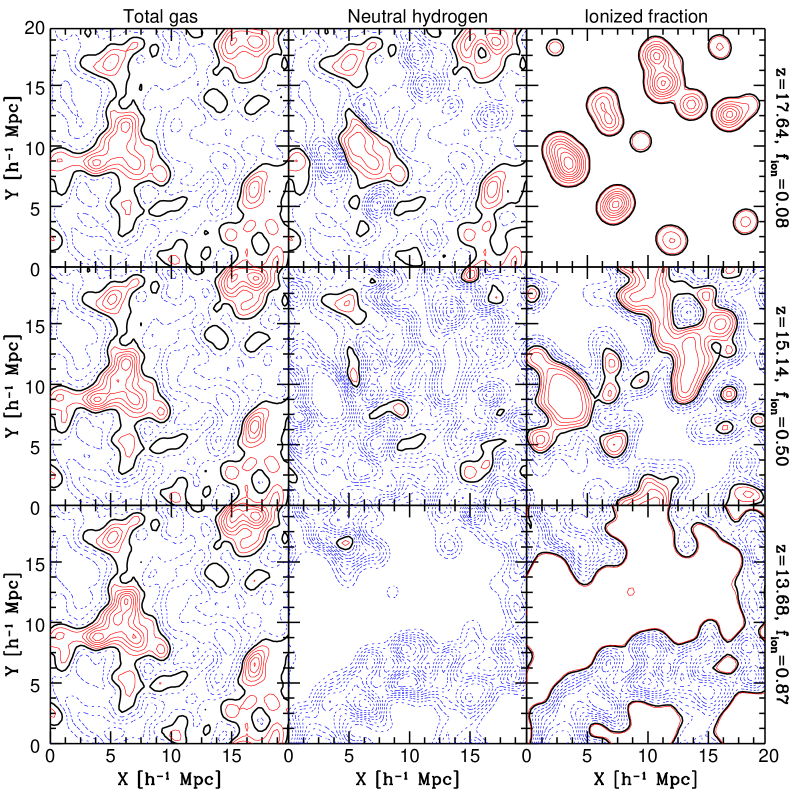
Figure 1: Fluctuations in the total gas density (left column), the H I density (middle column), and the ionized fraction $X_{{}_{\mbox{\scriptsize H\ {\tiny II}}}}=n_{{}_{\mbox{\scriptsize H\ {\tiny II}}}}/n_{{}_{\mbox{\scriptsize H}}}$ (right column) in a slice of the simulation box at $z=17.64$ (top), $z=15.14$ (middle row), and $z=13.68$ (bottom). The mean mass weighted ionized fractions, $f_{\rm ion}$, corresponding to these redshifts are indicated to the right of the figure. In the panels showing gas and H I fluctuations, the thick solid contour indicates the mean hydrogen density ${\bar{n}}_{{}_{H}}=2.66\times 10^{-7}\rm cm^{-3}$, while the thin solid and dotted contours, respectively, represent densities above and below ${\bar{n}}_{{}_{H}}$. The contour spacing in these panels is $0.1{\bar{n}}_{{}_{H}}$. In the panels showing $X_{{}_{\mbox{\scriptsize H\ {\tiny II}}}}$, the thick contour shows the value of $f_{\rm ion}$ and the thin solid and dotted contours, respectively, denote fractions above and below $f_{\rm ion}$. The contour spacing in the panels in the right column is 0.1.

Figure 2: MFs of excursions sets defined according to a threshold in the field $u=\ln(1+\delta_{{}_{\rm gas}})-\left<\ln(1+\delta_{{}_{\rm gas}})\right>$, where $\delta_{{}_{\rm gas}}$ is the gas density contrast smoothed with a Gaussian window of a width of $0.5\ {\rm h^{-1}Mpc}$. The squares are obtained from the gas distribution in the simulation at redshift $z=13.68$. The thick dotted lines represent the analytic expressions for Gaussian fields with $\lambda$ estimated from the field $u$. The thin solid lines are the MFs of ten Gaussian random fields realization with the power spectrum of the $\Lambda$CDM cosmology.

Figure 3: The MFs of gas (thick lines) and H I (thin lines) isodensity surfaces in the simulation. The gas and H I density fields are smoothed with a Gaussian window of $0.5\ {\rm h^{-1}Mpc}$ in width. Shown are results for redshifts, $z=17.64$ (solid lines), $15.14$ (dotted lines), and $13.68$ (dashed lines) corresponding to mass weighted mean ionized fraction of $f_{\rm ion}=0.08$, $0.5$, and $0.87$, respectively.

Let $u({\it\boldsymbol{x}})$ denote a scalar function of position, ${\it\boldsymbol{x}}$, defined in a 3D volume, $V$. Assume that $u$ has zero mean over the volume $V$ and let $\sigma$ be the r.m.s value given by $\sigma^{2}=\left<u^{2}\right>_{{}_{V}}$. Given a threshold value $u_{{}_{\rm thr}}$ we consider the excursion set $F_{\nu}$ formed by all points, ${\it\boldsymbol{x}}$, with $u({\it\boldsymbol{x}})\geq\nu\sigma$, where $\nu=u_{{}_{\rm thr}}/\sigma$. The global morphology of $u({\it\boldsymbol{x}})$ is then described by calculating the MFs as a function of $u_{{}_{\rm thr}}$. In 3D space there are four MFs, namely

$$V_{0}(\nu) = \frac{1}{V}\int_{V}{\rm d}^{3}x\Theta\left(\nu\sigma-u({\it\boldsymbol{x}})\right),$$ (1)

$$V_{1}(\nu) = \frac{1}{6V}\int_{\partial F_{\nu}}{\rm d}s,$$ (2)

$$V_{2}(\nu) = \frac{1}{6\pi V}\int_{\partial F_{\nu}}{\rm d}s\left[\kappa_{1}({\it\boldsymbol{x}})+\kappa_{2}({\it\boldsymbol{x}})\right],$$ (3)

$$V_{3}(\nu) = \frac{1}{4\pi V}\int_{\partial F_{\nu}}{\rm d}s\ \kappa_{1}({\it\boldsymbol{x}})\kappa_{2}({\it\boldsymbol{x}}),$$ (4)

where $\Theta$ is the Heaviside step function and, $\kappa_{1}$ and $\kappa_{2}$ are the principal curvatures (inverse of the principal radii) at a point ${\it\boldsymbol{x}}$ on the surface. The first MF, $V_{0}(\nu)$, is the total volume of the regions with $u$ above the threshold $u_{{}_{\rm thr}}=\nu\sigma$. The remaining three MFs are calculated by surface integration over the boundary, $\partial F$, of the excursion set, where ${\rm d}s$ denotes the surface element on $\partial F$. The MF $V_{1}$ is a measure of the surface area of the boundary, $V_{2}$ is the mean curvature over the surface, and $V_{3}$ is the Euler characteristic, $\chi$. Compared to a sphere, oblate (pancake-like) surfaces are characterized by a large surface area, $V_{1}$, and a small mean curvature, $V_{2}$. The Euler characteristic, $\chi$, can be expressed in terms of the genus, $g$, as $\chi=2(1-g)$, where a sphere has $g=0$ and a torus has $g=1$ (Coles, Davies & Pearson 1996; Gott, Weinberg & Melott 1987). The genus can also be viewed as the number of distinct ways an object can be sliced without being disconnected into disjoint parts. Hence, two separate spheres have $g=-1$ since they can be considered as an object already made of two disconnected parts. Note that, while the Euler characteristic, $\chi$, is additive, the genus is not so (e.g. Coles, Davies & Peterson 1996).

For a Gaussian random field in 3D, the average MFs per unit volume have the following analytic form (Schmalzing & Buchert 1997)

$$V_{0}(\nu)=\frac{1}{2}-\frac{1}{\sqrt{2\pi}}\int_{0}^{\nu}\exp\left(-\frac{x^{2}}{2}\right){\rm d}x,$$ (5a)

$$V_{1}(\nu)=\frac{2}{3}\frac{\lambda}{\sqrt{2\pi}}\exp\left(-\frac{1}{2}\nu^{2}\right),$$ (5b)

$$V_{2}(\nu)=\frac{2}{3}\frac{\lambda^{2}}{\sqrt{2\pi}}\nu\exp\left(-\frac{1}{2}\nu^{2}\right),$$ (5c)

$$V_{3}(\nu)=\frac{\lambda^{3}}{\sqrt{2\pi}}\left(\nu^{2}-1\right)\exp\left(-\frac{1}{2}\nu^{2}\right),$$ (5d)

where $\lambda=\sqrt{\sigma_{1}^{2}/6\pi\sigma^{2}}$, $\sigma\equiv\left<u^{2}\right>^{1/2}$, $\sigma_{1}\equiv\left<\left|\nabla u\right|^{2}\right>^{1/2}$.

Given a sampling of the field, $u({\it\boldsymbol{x}})$, on a discrete cubic lattice we use two methods to calculate the MFs (Schmalzing & Buchert 1997). The first method is based on Koenderink invariants (Schmalzing 1996; Koenderink 1984; ter Haar Romeny et al. 1991). In this method, the local curvatures are expressed in terms of geometric invariants formed from the first and second derivatives of the field. The second method is based on Crofton’s formula (Crofton 1868; Schmalzing & Buchert 1997), which requires counting of the number of grid points, edges, surfaces and cells within the excursion set. The appendix A contains a more detailed description of these methods. We have compared the MFs obtained from the application of the two methods on the gas and H I density fields in the simulations. When the fields are interpolated on a $128^{3}$ cubic grid using a simple cloud-in-cell algorithm, we find a difference of more than $50\%$ between the corresponding MFs. The difference between the results obtained with the two methods is reduced to $~{}\hbox to0.0pt{\raise 1.72218pt\hbox{$<$}\hss}{\lower 3.01385pt\hbox{$\sim$}}~{}10\%$ by smoothing the density fields with a Gaussian filter of $0.5\ {\rm h^{-1}Mpc}$ width. Therefore, we work with fields smoothed with a filter of $0.5\ {\rm h^{-1}Mpc}$. This filtering roughly corresponds to the instrumental resolution of LOFAR (Kassim et al. 2004). We have examined the difference between the methods using a finer grid of $256^{3}$ and obtained similar differences between the methods. The Koendernick invariants method, however, seems to be more robust and we only present results obtained with this method.

3 Simulations of IGM reionization

The simulation we adopt has been run by Ciardi, Ferrara & White (2003). This is a high-resolution numerical simulation that follows the evolution of the dark matter and diffuse gas distribution. It is combined to a semi-analytic model of galaxy formation which tracks the sources of ionization (Kauffmann et al. 1999), and to the Monte-Carlo radiative transfer code CRASH which follows the propagation of ionizing photons in the IGM (Ciardi et al. 2001; Maselli, Ferrara & Ciardi 2003). The simulation also assumes that the gas in the IGM consists only of hydrogen. The parameters are those of a $\Lambda$CDM “concordance” cosmology, with $\Omega_{m}=0.3$, $\Omega_{\Lambda}=0.7$, $h=0.7$, $\Omega_{b}=0.04$, $n=1$ and $\sigma_{8}=0.9$ (Spergel et al. 2003). The smallest resolved halos have a mass $M\simeq 10^{9}$ M_⊙, and start to form at $z\sim 20$. Each simulation output provides a mock catalogue of galaxies which are described, among others, by their position, star formation rate and UV emissivity. For the specific run considered here (labeled L20 in the original paper) reionization is completed by $z\sim 13$, and the associated Thomson scattering optical depth is $\tau_{\rm e}0.161$, consistent with the result from the first year WMAP data (Spergel et al. 2003). The total gas number density, $n_{{}_{\mbox{\scriptsize H}}}$, and the neutral gas number density, $n_{{}_{\mbox{\scriptsize H\ {\tiny I}}}}$, are provided on a cubic grid of $128^{3}$. Since we have found that MFs computed directly from the density fields sampled on a grid without any additional smoothing are rather noisy, we smooth the gas and H I density fields with a Gaussian filter of width of $0.5\ {\rm h^{-1}Mpc}$. All results will be presented for the smoothed fields. Using these fields, we compute the ionized fraction, $X_{{}_{\mbox{\scriptsize H\ {\tiny II}}}}=n_{{}_{\mbox{\scriptsize H\ {\tiny II}}}}/n_{{}_{\mbox{\scriptsize H}}}$ ($n_{{}_{\mbox{\scriptsize H\ {\tiny II}}}}=n_{{}_{\mbox{\scriptsize H}}}-n_{{}_{\mbox{\scriptsize H\ {\tiny I}}}}$), and the mass weighted mean ionized fraction, $f_{\rm ion}=\left<n_{{}_{\mbox{\scriptsize H}}}X_{{}_{\mbox{\scriptsize H\ {\tiny II}}}}\right>_{V}/\left<n_{{}_{\mbox{\scriptsize H}}}\right>_{V}$. Snapshots at redshift $z=17.64$, $z=15.14$, and $z=13.68$ will be used. These correspond to a mean ionized fraction $f_{\rm ion}=0.08$, $f_{\rm ion}=0.5$, and $f_{\rm ion}=0.87$, respectively.

Fig. 1 shows contour maps of the smoothed gas and H I density fluctuations (left and middle columns, respectively) at $z=17.64$ (top row), $z=15.14$ (middle row), and $z=13.68$ (bottom row). The figure also shows the ionized fraction, $X_{{}_{\mbox{\scriptsize H\ {\tiny II}}}}$ (right column). In the panels to the left, the increase in the contour levels as we go from the top to bottom is the result of the cosmological growth of fluctuations (e.g. Peebles 1980). Non-Gaussian features are already significant at those redshifts as indicated by the lack of symmetry between the distribution of regions with densities above and below the mean. A comparison between the left and middle columns shows significant differences between the morphology of the gas and H I distribution already at the initial stages of reionization when the mean ionized fraction is only $f_{\rm ion}=0.08$. At these stages, the maps of $X_{{}_{\mbox{\scriptsize H\ {\tiny II}}}}$ (right column) indicate that the ionized regions are mainly individual nearly spherical patches. Recombinations play an important role at $z=17.64$ and $15.14$ as inferred from the broad distribution of $X_{{}_{\mbox{\scriptsize H\ {\tiny II}}}}$ values (see also Ciardi & Madau 2003).

3.1 The morphology of the gas distribution

The evolved gas density field tends to have a lognormal probability distribution function (e.g. Theuns et al. 1998). Consequently, we expect the MFs of the log of the gas density field to be well approximated by the analytic expressions for Gaussian random fields (eqs. (5a), (5b), (5c) & (5d)). In Fig. 2, we present the MFs of $u=\ln(1+\delta_{{}_{\rm gas}})-\left<\ln(1+\delta_{{}_{\rm gas}})\right>$ where $\delta_{{}_{\rm gas}}$ is the smoothed gas density contrast obtained from the simulation output at $z=13.68$. There is an excellent match between the MFs in the simulation and the analytic expressions. For high density thresholds, the excursion sets are formed by individual density peaks each having an Euler characteristic equal to that of a sphere. In that regime, $V_{3}$ is therefore proportional to the number density of peaks above the threshold. Note that, in the case of a Gaussian field, the symmetric form of $V_{3}$ reflects the symmetry in the statistical properties of negative and positive peaks. Similar results were obtained at redshifts $z=17.64$ and $z=15.14$. As an estimate of the cosmic variance in the MFs measured from the L20 simulation, we compute the scatter around the mean MFs drawn from an ensemble of realizations of random fields with lognormal probability distribution function (PDF). Namely, Gaussian random realizations of the concordance $\Lambda$CDM power spectrum are generated in a periodic box of size $L=20\ {\rm h^{-1}Mpc}$. These Gaussian fields are mapped onto lognormal fields, which are then normalized to the r.m.s. value of smooth density fluctuations in the simulations. The MFs of 10 such lognormal realizations are plotted as the thin lines in Fig. 2. The deviations of these MFs from the analytic expressions (thick dotted lines) is the result of the finite size of the box. The deviations are most pronounced in $V_{3}$ which depends on $\sigma^{-3}$ (see eq. (5d)) and are smallest in $V_{0}$ which does not depends on $\sigma$ at all (see eq. (5a)).

3.2 The morphology of the H I distribution

Figure 4: The MFs of the neutral hydrogen density as a function of the mass weighted ionized fraction from the simulations. We present the results for four density thresholds: $n^{\rm thr}_{\mbox{\scriptsize H\ {\tiny I}}}=0.001\bar{n}_{\rm H}$ (solid lines), $n^{\rm thr}_{\mbox{\scriptsize H\ {\tiny I}}}=0.01\bar{n}_{\rm H}$ (dotted lines), $n^{\rm thr}_{\mbox{\scriptsize H\ {\tiny I}}}=0.1\bar{n}_{\rm H}$ (dashed lines),) and $n^{\rm thr}_{\mbox{\scriptsize H\ {\tiny I}}}=\bar{n}_{\rm H}$ (dot-dashed lines), where $\bar{n}_{\rm H}=2.66\times 10^{-7}\ {\rm cm^{-3}}$.

The reionization process in the simulation begins with the appearance of individual ionized patches generated by the propagation of UV ionization fronts originating from the earliest galaxies. During a later stage, when $f_{\rm ion}\sim 0.5$, the geometry of ionized regions transforms into a complex structure of tunnels and islands. Towards the end of the EoR, UV ionizing photons form a nearly uniform background which maintains most of the IGM at a local ionization level determined by the balance of photo-ionization with recombinations. In Fig. 3, we plot the MFs of the smoothed gas (thick lines) and H I (thin lines) number densities, for three redshifts. The deviations of the MFs of the H I distribution from those of the gas are already significant at $z=17.64$ when the ionized fraction is only $f_{\rm ion}=0.08$. Comparison between the thin (H I) and thick (gas) lines in the top-left panel shows that the highest density regions are all ionized. At $z=17.64$, all regions with density $~{}\hbox to0.0pt{\raise 1.72218pt\hbox{$>$}\hss}{\lower 3.01385pt\hbox{$\sim$}}~{}1.42{\bar{n}}_{{}_{\rm H}}$ are ionized together with some moderate density regions, whereas at $z=13.68$, all the regions with mean densities and above are ionized. Between $z=17.64$ and $z=15.14$ significant reionization occurs in regions of densities below the mean (compare solid and dotted thin lines). The MFs at the three redshifts are substantially different, making the MFs a good discriminator of the various stages of reionization. In Fig. 4, we examine the evolution of the MFs of the H I distribution as a function of the mass weighted ionized fraction, $f_{\rm ion}$, for the density thresholds: $n^{\rm thr}_{\mbox{\scriptsize H\ {\tiny I}}}=0.001\bar{n}_{\rm H}$ (solid lines), $n^{\rm thr}_{\mbox{\scriptsize H\ {\tiny I}}}=0.01\bar{n}_{\rm H}$ (dotted lines), $n^{\rm thr}_{\mbox{\scriptsize H\ {\tiny I}}}=0.1\bar{n}_{\rm H}$ (dashed lines), and $n^{\rm thr}_{\mbox{\scriptsize H\ {\tiny I}}}=\bar{n}_{\rm H}$ (dot-dashed lines), where the mean gas density is $\bar{n}_{\rm H}=2.66\times 10^{-7}\ {\rm cm^{-3}}$. As expected, the volume functional, $V_{0}(\nu)$, decreases with $f_{\rm ion}$. At the initial stages of reionization, the ionized volume of space is made of non-overlapping patches, so that the surface area, $V_{1}$, is an increasing function of $f_{\rm ion}$, and the integrated mean curvature functional, $V_{2}(\nu)$, is negative . When the ionized fraction $f_{\rm ion}$ becomes significant, the behaviour of $V_{1}$, $V_{2}$, and the Euler characteristic $V_{3}$, is reversed compared to their behaviour at low $f_{\rm ion}$. The reason is that both the ionized volume in the early phase of reionization, and the neutral volume in the late stages, are predominantly made of individual patches and, therefore, share similar topological properties.

4 Semi-analytic modeling of the morphology of reionization

Figure 5: Comparison of the MFs of the smoothed H I density field from the simulation with those obtained from the recipes A, B, C, D, E, & F. Left, middle and right columns correspond to $z=17.64$, $z=15.14$, and $z=13.68$, respectively. The thick solid lines represent the MFs from the H I distribution in the simulation. The thick dotted corresponds to recipe A, thick dashed to B, thin solid to C, thin dashed to D, thin long-dashed to E, and dash-dotted to F. The best match to the simulation is obtained with B (thick dashed).

Figure 6: The same as the previous figure, but with recipes A–F applied to a lognormal random density field in a cubic box of $50\ {\rm h^{-1}Mpc}$ on the side. Here also, recipe B (thick dashed) yields the best match to the MFs from H I field in the simulation (thick solid).

4.1 Modeling the morphology in the simulation

Our goal here is twofold. First, we will attempt to reproduce the MFs of the H I distribution in the simulation using simple recipes that do not require explicit treatment of radiative transfer. Second, given these recipes we will assess the extent to which MFs can discriminate between reionization scenarios other than those adopted in the particular simulation used here. In the recipes A, B, C, and D, that we describe below, the H I distribution is obtained by overlaying the gas distribution with spherical bubbles devoid of neutral gas, while the surrounding gas is kept neutral. In the recipes E and F the IGM in the simulation box is ionized cell by cell as explained below. All the models assume that a grid cell is either completely ionized or neutral. Clearly, this is an oversimplification especially in the early stages of reionization (see column to the right in Fig. 1). Yet we will see that one of these recipes indeed reproduces the MFs measured in the simulations. We now summarize the different recipes.

• A: spherical bubbles are placed randomly in the simulation. All bubbles have the same radius, $R$, independent of local gas density.

• B: the same as A, but with bubble radius, $r$, depending on the local density. We have tried several functional forms, and found that the following parametrization gives the best match to the MFs of the simulation,

  $$r({\it\boldsymbol{x}})=\left\{\begin{array}[]{ll}R+6R\left[1-\left(1+\delta({\it\boldsymbol{x}})\right)^{-1/3}\right]&1+\delta\geq\left(6/7\right)^{3}\\ 0&1+\delta<\left(6/7\right)^{3}\end{array}\right.,$$ (6)

  where $\delta({\it\boldsymbol{x}})$ is the smoothed density contrast at the position ${\it\boldsymbol{x}}$, and $R$ is a constant.

• C: bubbles of fixed radius $R$, are added one by one, where a newly added bubble is centered on the highest density grid point not encompassed by previous bubbles.

• D: the same as C but with new bubbles centered at lowest density point.

• E: grid cells are ionized according to their density, starting from the cell with the highest gas density.

• F: the same as E but starting from the lowest density cell.

We apply each of the recipes described above to the gas distribution in the L20 simulation. To facilitate the comparison with the MFs derived from the H I distribution in the simulation, the number of bubbles in A–D, and the number of ionized cells in E & F are tuned so that the mean mass weighted ionized fraction matches the value measured in the simulation at a given redshift. In Fig. 5, we compare the MFs obtained with these recipes to those of the actual H I distribution in the simulation. Left, middle, and right columns show, respectively, results for $z=17.64$, 15.14, and 13.88. In each of the models A–D, the parameter $R$ is tuned to the value giving the best match to the curve of $V_{0}$ obtained from the simulation. We have found that this value mainly depends on redshift: $R=0.94$, 1.56, and $2.03\ {\rm h^{-1}Mpc}$ comoving for $z=17.64$, 15.14, and 13.88, respectively. The figure shows results for these values of $R$ only. Recipe B (thick dashed lines) yields the best fit to the MFs of the actual H I distribution in simulation (think solid lines). In this model, the radius of bubbles in regions with overdensities $~{}\hbox to0.0pt{\raise 1.72218pt\hbox{$<$}\hss}{\lower 3.01385pt\hbox{$\sim$}}~{}0.63$ is practically zero. Therefore, these regions are only ionized by sources in nearby denser regions. This reflects the relative lack of ionizing sources (galaxies) in the voids of the simulation volume.

The numerical simulation we use has a relatively small box ($20\ {\rm h^{-1}Mpc}$) so that cosmic variance may introduce large uncertainties in the estimates of the MFs (see thin lines in Fig. 2). Furthermore, it is assumed in this simulation that reionization is caused solely by UV radiation. The amount of UV photons emitted by a “galaxy” in the simulation is sensitive to the adopted parameters of the semi-analytic galaxy formation model. The distribution of the “galaxies”, which greatly affects the development of the early stages, also depends on the galaxy formation model. Exploring the parameter space of the galaxy formation model and all possible scenarios with large volume simulations is currently unfeasible. Nonetheless, Figs. 5 demonstrate that the MFs can distinguish between the different reionization scenarios examined here.

To reduce the effect of cosmic variance in the MFs we apply the recipes A–F to lognormal random fields in a cubic box of $50\ {\rm h^{-1}Mpc}$ on the side (more than 15 times the volume of the L20 simulation). The corresponding MFs are shown in Fig. 6. The larger box size significantly reduces the noise in the MFs, especially for $V_{3}$. In general, there are only minor differences between Figs. 5 and 6, indicating that the lognormal approximation yields results in agreement with the simulation. This is expected since the morphology of the total gas density is well approximated by the MFs of a lognormal field. Therefore, the morphology of reionization can also be modeled using lognormal fields without resorting to detailed simulations.

4.2 Morphology in an X-ray pre-reionization scenario

Figure 7: MFs of excursions sets obtained from the H I distribution in an X-ray pre-reionization scenarios. Plotted are curves for three values of $X_{{}_{\mbox{\scriptsize H\ {\tiny I}}}}$ at mean gas density, as indicated in the figure. All curves are for $z=17.64$.

Figure 8: The MFs from the previous figure plotted against threshold in $\nu=\left[\ln(n_{{}_{\mbox{\scriptsize H\ {\tiny I}}}})-\left<\ln(n_{{}_{\mbox{\scriptsize H\ {\tiny I}}}})\right>\right]/\sigma$ where $\sigma^{2}=\left<\left[\ln(n_{{}_{\mbox{\scriptsize H\ {\tiny I}}}})-\left<\ln(n_{{}_{\mbox{\scriptsize H\ {\tiny I}}}})\right>\right]^{2}\right>$. The analytic MFs for Gaussian random field are shown as the dash-dotted lines.

Reionization by UV sources can be preceded by a pre-reionization epoch in which the gas is partially ionized by an X-ray background produced by accretion onto mini black holes (Ricotti & Ostriker 2004). The mean free path of X-ray photons is much larger than both the correlation length and the mean separation of the sources. Therefore, in this scenario, X-ray photons act as a uniform ionizing background and the H I fraction, $X_{{}_{\mbox{\scriptsize H\ {\tiny I}}}}=n_{{}_{\mbox{\scriptsize H\ {\tiny I}}}}/n_{{}_{\mbox{\scriptsize H}}}$, at a point with density contrast $\delta$, is determined by the equation for photo-ionization equilibrium,

$$\Gamma X_{{}_{\mbox{\scriptsize H\ {\tiny I}}}}=\alpha_{\mbox{\scriptsize H\ {\tiny I}}}^{(2)}{\bar{n}}(1+\delta)(1-X_{{}_{\mbox{\scriptsize H\ {\tiny I}}}})^{2}\;,$$ (7)

where $\Gamma$ is the X-ray photo-ionization rate per hydrogen atom, $\alpha_{\mbox{\scriptsize H\ {\tiny I}}}^{(2)}$ is the recombination cross section to the second excited atomic level, $\bar{n}$ is the mean density of total (ionized plus neutral) hydrogen, and $X_{{}_{\mbox{\scriptsize H\ {\tiny I}}}}$ is the H I fraction. According to Ricotti & Ostriker (2004), the mean H I fraction should be maintained at a level $X_{{}_{\mbox{\scriptsize H\ {\tiny I}}}}\sim 0.8-0.9$ in the redshift range $20~{}\hbox to0.0pt{\raise 1.72218pt\hbox{$<$}\hss}{\lower 3.01385pt\hbox{$\sim$}}~{}z~{}\hbox to0.0pt{\raise 1.72218pt\hbox{$<$}\hss}{\lower 3.01385pt\hbox{$\sim$}}~{}40$ in order to yield a large optical depth $\tau_{\rm e}\sim 0.1$. This level of reionization is ideal for producing a significant 21-cm signal (Nusser 2005a; Kuhlen, Madau & Montgomery 2006). In order to model the MFs of H I isodensity surfaces in this scenario, we use the lognormal gas density fields which have been computed from Gaussian random fields in a box of $50\ {\rm h^{-1}Mpc}$ on the side. We fix the ratio $\alpha_{\mbox{\scriptsize H\ {\tiny I}}}^{(2)}{\bar{n}}/\Gamma$ by assuming that $X_{{}_{\mbox{\scriptsize H\ {\tiny I}}}}$ is given at mean density, i.e. at $\delta=0$. Then, for any $\delta$, $X_{{}_{\mbox{\scriptsize H\ {\tiny I}}}}$ can be easily found using eq. (7). In Fig. 7 we present the MFs of excursions sets obtained from X-ray background H I fields at redshift $z=17.64$ for values of the H I fraction at mean density of $X_{{}_{\mbox{\scriptsize H\ {\tiny I}}}}=0.95$ (solid lines), 0.9 (dotted lines), and 0.8 (dashed lines). Changing the H I fraction shifts the MFs horizontally, but does not affect their overall shape. This is not surprising since all these models have similar topologies. In Fig. 8, we plot the MFs as functions of excursion sets obtained from the field $\ln(n_{{}_{\mbox{\scriptsize H\ {\tiny I}}}})$. Also plotted, as the dash-dotted lines, are the analytic expressions for Gaussian random field. The figure demonstrates that for the low levels of ionization obtained in X-ray pre-reionization, the MFs of the H I distribution are close to those of a lognormal field which also describes the morphology of the gas distribution in our case.

5 Discussion

Among all possible measures of global morphology, only Minkowski Functionals (MFs) are invariant under rotational and translational transformations (Hadwiger 1957). But can the MFs distinguish between various stages of EoR or between different reionization scenarios? We have assessed this question using a high-resolution numerical simulation in which reionization is driven by UV photons emitted from stellar type sources and by employing simple recipes to describe different reionization scenarios. We have found that the MFs of isodensity surfaces of the gas distribution in the simulation are well described by those of a field having a lognormal distribution function. In a UV reionization scenario, the deviations from the lognormal MFs are sensitive to the distribution of ionized regions. The MFs of the H I distribution depend on a multitude of factors among which are: the gas density field and its correlation with the distribution of ionizing sources, the abundance of sources, and the intensity and type (UV versus x-rays) of the emitted radiation. Reionization by UV begins with individual patches appearing around sources associated with the most massive and rarest haloes (e.g. Benson et al. 2005). The topology of reionization in these early stages is substantially different from that of later stages when ionized regions form a complex network of tunnels in addition to isolated patched. This difference in topology is reflected in the shapes of the MFs. X-rays have a substantially larger mean free path than UV photons. Therefore, x-rays generated by an early generation of black holes that tend to form a uniform background that may partially ionize the IGM. We have considered the MFs of the H I distribution in an epoch of pre-reionization caused by an x-ray background. Using a semi-analytic modeling of this epoch, we find similar H I and gas topologies. This is due to the low local ionized fractions obtained in these models.

Despite the complexity of the reionization process as given by the simulation (cf. Ciardi, Ferrara & White 2003), its topology can be described using simple semi-analytic recipes that do not involve a detailed treatment of radiative transfer. Application of some of these recipes on lognormal random fields yield a good match to the MFs obtained from the simulation. However, one may envisage a variety of alternative UV reionization scenarios (e.g. Miralda-Escudé, Haehnelt & Rees 2000), depending on the details of galaxy formation and the dark matter distribution. It therefore remains to be confirmed whether semi-analytic recipes can actually match the MFs obtained from detailed simulations of alternative scenarios corresponding to physical assumptions different from those adopted in the simulation we have used in this paper.

In the near future, the next generation of radio telescopes will provide maps of twenty-one centimeter (21-cm) line from neutral IGM and probe the three dimensional distribution of H I during the EoR. It will be then possible to use MFs to study the morphology of the reionization process as described in this work. However, the observed 21-cm maps will be affected by redshift distortions (e.g. Ali, Bharadawaj & Pandey 2005; Barkana & Loeb 2005; Nusser 2005b), instrumental noise, and foreground contamination. The usefulness of MFs derived from 21-cm maps which include all these effects has yet to be demonstrated. This will be the subject of future work in which the modified methodology of Benson et al. (2001, 2005) for studying reionization will be implemented in a high resolution N-body simulation of a large box ($\sim 140\ {\rm h^{-1}Mpc}$ on the side).

The background density parameters and the value of $\sigma_{8}$ of the simulation used in this paper are consistent with the first year WMAP data (Spergel et al. 2003). Although the third year WMAP data give similar values for the density parameters as the first year data, it yields $\sigma_{8}=0.74^{+0.05}_{-0.06}$ and $\tau_{\rm e}=0.09^{+0.03}_{-0.03}$ (Spergel et al. 2006). The difference in the values for $\sigma_{8}$ and $\tau_{\rm e}$ can amount to substantial changes in the reionization history (Benson et al. 2005). This work has been completed before the the third year data has been published and therefore simulations have been run with cosmological parameters inferred from the first year WMAP data. Nevertheless, our aim at this stage is to illustrate the use of MFs for studying the history of cosmic reionization. Implications of MFs of 21-cm maps generated from a suite of simulations will be presented elsewhere.

Auto-correlations estimated from 21-cm maps have also been proposed as a statistical measure of H I distribution. The advantage of auto-correlations is that redshift distortions, noise, and foreground contamination can probably be easily incorporated in or removed from them, while these effects might play a more important or ambiguous role in MFs of 21-cm maps. Nevertheless, as auto-correlations are insensitive to morphology (e.g. a Gaussian random field and another highly non-Gaussian one, can have identical auto-correlation functions), MFs are better discriminators between different reionization scenarios. Therefore, an exploration of MFs of 21-cm maps is worthwhile.

Appendix A Numerical calculation of the Minkowski functionals

Schmalzing & Buchert (1997) used an integral geometry approach and developed two numerical methods to investigate the morphology of a sampled density field on a cubic lattice grid. Using the techniques pioneered by Koenderink (Koenderink 1984; ter Haar Romeny et al. 1991) in two-dimensions, Schmalzing (1996) expressed the local curvatures in term of geometric invariants formed from first and second derivatives. These invariants are known as the Koenderink invariants.

$$\kappa_{1}+\kappa_{2}=\frac{\epsilon_{ijm}\epsilon_{klm}u_{,i}u_{,jk}u_{,l}}{(u_{,n}u_{,n})^{3/2}},$$ (8a)

$$\kappa_{1}\kappa_{2}=\frac{\epsilon_{ijk}\epsilon_{lmn}u_{,i}u_{,l}u_{,jm}u_{,kn}}{2(u_{,p}u_{,p})^{2}},$$ (8b)

where $\kappa_{1}$ and $\kappa_{2}$ are the principal curvatures, $u({\bf x})$ is a three-dimensional density field in a box of a volume $V$, $u_{,i}$ and $u_{,ij}$ are the first and second spatial derivatives of the field $u({\it\boldsymbol{x}})$ respectively in the $i$ and $j$ directions, and $\epsilon_{ijk}$ is the Levi-Civita tensor.

Since one can replace the surface integration in eqs. (2), (3) & (4) with a spatial mean over the whole volume, the MFs become

$$V_{1}(\nu)=\frac{1}{6V}\int_{V}{\rm d}^{3}x\delta(\nu\sigma-u({\it\boldsymbol{x}}))\left|\nabla u({\it\boldsymbol{x}})\right|,$$ (9a)

$$V_{2}(\nu)=\frac{1}{6\pi V}\int_{V}{\rm d}^{3}x\delta(\nu\sigma-u({\it\boldsymbol{x}}))\left|\nabla u({\it\boldsymbol{x}})\right|\left[\kappa_{1}({\it\boldsymbol{x}})+\kappa_{2}({\it\boldsymbol{x}})\right],$$ (9b)

$$V_{3}(\nu)=\frac{1}{4\pi V}\int_{V}{\rm d}^{3}x\delta(\nu\sigma-u({\it\boldsymbol{x}}))\left|\nabla u({\it\boldsymbol{x}})\right|\kappa_{1}({\it\boldsymbol{x}})\kappa_{2}({\it\boldsymbol{x}}),$$ (9c)

where $\nu$ is the density threshold divided by the field r.m.s. value, $\sigma$, and $\delta$ is a delta function.

The second method is based on Crofton’s formula (Crofton 1868) which requires counting of the number of grid points, edges, surfaces and cells within the excursion set. The MFs in three-dimensions are given by

$$V_{0}(K)=\frac{1}{L}N_{3}(K),$$ (10a)

$$V_{1}(K)=\frac{2}{9}\frac{1}{aL}\left[-3N_{3}(K)+N_{2}(K)\right],$$ (10b)

$$V_{2}(K)=\frac{2}{9}\frac{1}{a^{2}L}\left[3N_{3}(K)-2N_{2}(K)+N_{1}(K)\right],$$ (10c)

$$V_{3}(K)=\frac{1}{a^{3}L}\left[-N_{3}(K)+N_{2}(K)-N_{1}(K)+N_{0}(K)\right],$$ (10d)

where the body $K$ is the excursion set of a homogeneous and isotropic random field sampled at $L$ points of a cubic lattice of spacing $a$. $N_{3}(K)$ gives the number of cubes within the body, $N_{2}(K)$ is the number of faces and $N_{1}(K)$ is the number of edges of the lattice cubes which belong to the body, while $N_{0}(K)$ gives the number of lattice points contained in $K$.

In http://physics.technion.ac.il/~lirong/mfs.tar.gz one can find the MFs software package for MFs calculation. This package includes the Koenderink invariants method, the Crofton’s formula method and the analytical calculation for Gaussian random field.

References

- [1] Ali Sk. S., Bharadwaj S., Pandey B., 2005, MNRAS, 363, 251
- [2] Barkana R., Loeb A., 2005, ApJ, 626, 1
- [3] Becker R. H. et al. , 2001, AJ, 122, 2850
- [4] Benson A. J., Nusser A., Sugiyama N., Lacey, C.G., 2001, MNRAS, 320, 153
- [5] Benson, A. J., Sugiyama N., Nusser A., Lacey C. G., 2006, MNRAS, 369, 1055
- [6] Bowman J. D., Morales M. F., Hewitt J. N., 2006, ApJ, 638, 20
- [7] Carilli C. L., Furlanetto, S., Briggs F., Jarvis M., Rawlings S., Falcke H., 2004a, NewAR, 48, 1029
- [8] Carilli C. L., Gnedin N., Furlanetto S., Owen F., 2004b, NewAR, 48, 1053
- [9] Ciardi B., Ferrara A., Marri S., Raimondo G., 2001, MNRAS, 324, 381
- [10] Ciardi B., Madau P., 2003, ApJ, 596, 1
- [11] Ciardi B., Ferrara A., White S. D. M., 2003, MNRAS, 344, L7
- [12] Coles P., Davies A. G., Pearson R. C., 1996, MNRAS, 281, 1375
- [13] Croft R. A. C., Weinberg D. H., Bolte M., Burles S., Hernquist L., Katz N., Kirkman D., Tytler D., 2002, ApJ, 581, 20
- [14] Crofton M. W., 1868, Philos. Trans. R. Soc. London, A, 158, 181
- [15] Desjacques V., Nusser A., 2005, MNRAS, 361, 1257
- [16] Di Matteo T., Ciardi B., Miniati F., 2004, MNRAS, 355, 1053
- [17] Eriksen H. K., Novikov D. I., Lilje P. B., Banday A. J., G rski K. M., 2004, ApJ, 612, 64
- [18] Gott J. R. III, Weinberg D.H., Melott A. L., 1987, ApJ, 319, 1
- [19] Gunn J.E., Peterson B.A., 1965, ApJ, 142, 1633
- [20] Hadwiger H., 1957, Vorlesungen über Inhalt, Oberfläche und Isoperimeterie (Berlin: Springer)
- [21] Kassim N. E., Lazio T. J. W., Ray P. S., Crane P. C., Hicks B. C., Stewart K. P., Cohen A. S., Lane, W. M., 2004, P&SS, 52, 1343
- [22] Kauffmann G., Colberg J. M., Diaferio A., White S. D. M., 1999, MNRAS, 307, 529
- [23] Kerscher M., Schmalzing J., Retzlaff J., Borgani S., Buchert T.,Gottlöber S., Müller V., Plionis M., Wagner H., 1997, MNRAS, 284, 73
- [24] Kerscher M., Schmalzing J., Buchert T., Wagner H., 1998, A&A, 333, 1
- [25] Kerscher M., Mecke K., Schmalzing J., Beisbart C., Buchert T., Wagner H., 2001, A&A, 373, 1
- [26] Koenderink J. J., 1984, Biol. Cybern., 50, 363
- [27] Komatsu E. et al. , 2003, ApJS, 148, 119
- [28] Kuhlen M., Madau P., Montgomery R., 2006, ApJ, 637, 1
- [29] Maselli A., Ferrara A., Ciardi B., 2003, MNRAS, 345, 379
- [30] McDonald P. et al. , 2005, ApJ, 635, 761
- [31] Mecke K. R., Buchert T., Wagner H., 1994, A&A, 288, 697
- [32] Miralda-Escudé J., Haehnelt M., Rees M. J. 2000, ApJ, 530, 1
- [33] Novikov, D., Schmalzing, J., Mukhanov, V. F., 2000, A&A, 364, 17
- [34] Nusser A., Haehnelt M., 2000, MNRAS, 313, 364
- [35] Nusser A., Benson A. J., Sugiyama N., Lacey C., 2002, ApJ, 580, 93
- [36] Nusser A., 2005a, MNRAS, 359, 183
- [37] Nusser A., 2005b, MNRAS, 364, 743
- [38] Oh S. P., Mack K. J., 2003, MNRAS, 346, 8710
- [39] Peebles P. J. E., 1980, The Large-Scale Structure of the Universe, Princeton University Press
- [40] Pen U. L., Wu X. P., Peterson J., 2004, Chin. J. Astron. Astrophys.,submitted (astro-ph/0404083)
- [41] Percival, W. J. et al. , 2002, MNRAS, 337, 1068
- [42] Peterson J., Pen U. L., Wu X. P., 2006, in Kassim N., Perez M., Junor M., Henning P., eds, Astron. Soc. Pac. Conf. Ser. Vol 345, From Clark Lake to the Long Wavelength Array: Bill Erickson’s Radio Science, Astron. Soc. Pac., San Francisco, p. 441
- [43] Räth C., Schuecker P., 2003, MNRAS, 344, 115
- [44] Ricotti, M., Ostriker, J.P., 2004, MNRAS, 352, 547
- [45] Schmalzing J., 1996, Diplomarbeit, Ludwig-Maximilian-Universität, München
- [46] Schmalzing J., Buchert T., 1997, ApJ, 482, L1
- [47] Schmalzing J., Gorski K. M., 1998, MNRAS, 297, 355
- [48] Schmalzing J., Takada M., Futamase T., 2000, ApJ, 544, 83
- [49] Shandarin S. F., Feldman H. A., Xu Y., Tegmark M., 2002, ApJS, 141, 1
- [50] Spergel D. N. et al. , 2003, ApJS, 148, 175
- [51] Spergel D. N. et al. , 2006, ApJ, submitted (astro-ph/0603449)
- [52] ter Haar Romeny B. M., Florack L. M. J., Koenderink J. J., Viergever M. A., 1991, in Colchester A. C. F., Hawke D. J., eds, Lecture Notes of Computer Science, Vol. 511, Scale Space: Its Natural Operators and Differential Invariants. Springer-Verlag, Berlin, p. 239
- [53] Theuns T., Leonard A., Schaye J., Efstathiou G., 1998, MNRAS, 303, 58
- [54] Tytler T. et al. , 2004, ApJ, 617, 1
- [55] Zaroubi S., Viel M., Nusser A., Haehnelt M., Kim T. -S., 2006, MNRAS, 369, 734
- [56] Zehavi I., 2002, ApJ, 571, 172