The Absence of Adiabatic Contraction of the Radial Dark Matter
Profile in the Galaxy Cluster A2589

Abstract

We present an X-ray analysis of the radial mass profile of the radio-quiet galaxy cluster A2589 between $0.015-0.25\,\rm{r_{vir}}$ using an XMM-Newton observation. Except for a $\approx 16$ kpc shift of the X-ray center of the $R=45-60$ kpc annulus, A2589 possesses a remarkably symmetrical X-ray image and is therefore an exceptional candidate for precision studies of its mass profile by applying hydrostatic equilibrium. The total gravitating matter profile is well described by the NFW model (fractional residuals $\lesssim 10\%$) with $c_{\rm vir}=6.1\pm 0.3$ and $M_{\rm vir}=3.3\pm 0.3\times 10^{14}M_{\odot}$ ($r_{vir}=1.74\pm 0.05$ Mpc) in excellent agreement with $\Lambda$CDM. When the mass of the hot ICM is subtracted from the gravitating matter profile, the NFW model fitted to the resulting dark matter (DM) profile produces essentially the same result. However, if a component accounting for the stellar mass ($M_{*}$) of the cD galaxy is included, then the NFW fit to the DM profile is substantially degraded in the central $r\sim 50$ kpc for reasonable $M_{*}/L_{V}$. Modifying the NFW DM halo by adiabatic contraction arising from the early condensation of stellar baryons in the cD galaxy further degrades the fit. The fit is improved substantially with a Sersic-like model recently suggested by high resolution N-body simulations but with an inverse Sersic index, $\alpha\sim 0.5$, a factor of $\sim 3$ higher than predicted. We argue that neither random turbulent motions nor magnetic fields can provide sufficient non-thermal pressure support to reconcile the XMM mass profile with adiabatic contraction of a CDM halo assuming reasonable $M_{*}/L_{V}$. Our results support the scenario where, at least for galaxy clusters, processes during halo formation counteract adiabatic contraction so that the total gravitating mass in the core approximately follows the NFW profile.

1. Introduction

The properties of dark matter (DM) halos are a powerful discriminator between different cosmological models. Of particular importance is the distribution of halo concentration ($c_{\rm vir}$) with virial mass ($M_{\rm vir}$). For the concordance cold dark matter ($\Lambda$CDM) cosmology the mean $c_{\rm vir}$ varies slowly over a factor of 100 in $M_{\rm vir}$, whereas the scatter remains very nearly constant (e.g., Bullock et al., 2001; Kuhlen et al., 2005). At fixed halo mass, the distribution of concentrations is expected to vary significantly as a function of the cosmological parameters, including $\sigma_{8}$, $n$, and $w$, the dark energy equation of state (e.g. Dolag et al., 2004; Kuhlen et al., 2005).

The radial density profiles of CDM halos are fairly well described between approximately $0.01-1\,{\hbox{$r_{\rm vir}$}}$ (where $r_{\rm vir}$ is the virial radius) by the 2-parameter “NFW” model suggested by Navarro et al. (1997). More recent numerical simulations with higher resolution show that CDM halos deviate slightly from this average NFW profile because the density slope changes continuously with radius (e.g., Navarro et al., 2004; Diemand et al., 2004; Graham & et al., 2005). However, there is not yet a general consensus on whether the central density slope is shallower or steeper than the NFW profile.

The central regions of DM halos also reveal vital information about the interaction between the stellar baryons and the DM during halo formation. If the stellar baryons condense much earlier than the dissipationless DM, it is expected that the baryons will adiabatically compress the DM halo away from its pure NFW form (e.g., Blumenthal et al., 1986; Gnedin et al., 2004). It has also been argued that heating of the dark matter by dynamical friction with member galaxies counteracts adiabatic compression and leads to a total gravitating mass profile consistent with the pure NFW profile (e.g., El-Zant et al. 2004; see also Loeb & Peebles 2003).

In theory, galaxy clusters are excellent sites to study DM profiles, particularly in their cores, because they are DM-dominated deep down to a small fraction of the virial radius($\approx 0.007{\hbox{$r_{\rm vir}$}}$; e.g., Dubinski, 1998; Lewis et al., 2003) and several powerful techniques exist to probe cluster mass profiles. In practice, however, it has proven quite difficult to obtain precise, reliable measurements of the DM profiles in cluster cores. Stellar dynamical studies suffer from the long-standing and well-known problem of velocity dispersion anisotropy, and despite occasional claims to the contrary (e.g., Sand et al., 2004), cannot obtain precise constraints without restrictive assumptions on the form of the velocity dispersion tensor, and therefore of the mass profile. Since the weak lensing approximation breaks down within the central $\approx 100$ kpc of clusters, only those clusters with giant arcs produced by strong lensing can be used to map the core mass distribution. Unfortunately, giant arcs are preferentially produced in clusters with significant substructure in the core, making them much less suitable for comparison to the average relaxed cluster profile predicted by simulations.

X-ray observations of the hot intracluster medium (ICM) are a powerful probe of the DM in galaxy clusters (e.g., see recent reviews by Buote, 2004; Arnaud, 2005). Since the pressure tensor of the hot ICM is isotropic, and the gas traces the three-dimensional cluster potential well within the virial radius, X-ray observations are a vital complement to gravitational lensing techniques that probe only the projected potential. However, the X-ray method requires the ICM to be in approximate hydrostatic equilibrium. Morphological studies of X-ray images have shown that a large fraction of nearby clusters ($z<0.2$) do have regular image morphologies and appear to be nearly relaxed on 0.5-1 Mpc scales (e.g., Mohr et al., 1995; Buote & Tsai, 1996; Jones & Forman, 1999), though no cluster is observed to be (or is expected to be) devoid of evidence of disturbance.

Precisely how departures from hydrostatic equilibrium translate to errors in mass estimates is as yet not well understood in terms of quantifiable measures of the X-ray image morphology, projected temperature, or projected metallicity maps. What is clear is that errors in mass estimates should be minimized for clusters without obvious substructure (Tsai et al., 1994; Buote & Tsai, 1995; Evrard et al., 1996, though see Hallman et al. 2005). That is, clusters with regular X-ray isophotes, centrally peaked cores and no central AGN-induced disturbance. Further evidence for a relaxed hot ICM is suggested by a temperature profile that rises with radius from a minimum in the cluster core (e.g., De Grandi & Molendi, 2002) and by metallicity profile that is peaked at the center and declines monotonically with increasing radius (e.g., De Grandi et al., 2004; Böhringer et al., 2004).

Unfortunately, it has proven difficult to find cluster candidates that are relaxed both on large ($\approx 0.5-1$ Mpc) scales and within their cores because evolved, cool-core clusters typically have X-ray and radio disturbances within their cores believed to arise from AGN feedback (e.g., Bîrzan et al., 2004). A small number of radio-quiet clusters, previously classified as cooling flows, have been observed with Chandra; A2589 (Buote & Lewis, 2004), A644 (Buote et al., 2005), A1650 and A2244 (Donahue et al., 2005). None of these clusters displays the central minimum in the temperature profile characteristic of cool-core clusters or has any evidence for AGN feedback. The lack of AGN evidence for current feedback in these systems may arise from heating due to merging (Buote et al., 2005) or unusually powerful AGN feedback events in the distant past (Donahue et al., 2005).

The cluster A2589 ($z=0.0414$) is observed to be one of the most morphologically regular clusters in terms of its X-ray emission on a scale of $\approx 0.5$ Mpc (Buote & Tsai, 1996). The high-resolution Chandra image confirmed a highly symmetrical X-ray image morphology down to the center, although with some evidence for a small isophotal center shift of $\sim 10$ kpc. The highly regular X-ray image morphology combined with no evidence for AGN feedback make this cluster an excellent candidate for studies of its mass profile by making the approximation that the hot gas is in hydrostatic equilibrium. Because of the low photon statistics of our shallow Chandra observation we were unable to place strong constraints on the mass profile, though an NFW profile was found to be consistent with the data within $r\sim 150$ kpc.

In this paper we improve upon our previous study by using a higher quality XMM-Newton observation to extend our analysis to $\sim 400\,\rm{kpc}$ corresponding roughly to $\sim 1/4\,\rm{r_{vir}}$. The higher quality data will allow us to test different mass profiles proposed so far in the literature to account for the dark matter and the influence of the central bright dominant galaxy.

Our assumed virial radius is defined as the radius of a sphere whose mean density is 104.7 times the critical density of the universe. This value is estimated at the redshift of the cluster and for an $(\Omega_{m},\Omega_{\Lambda})=(0.3,0.7)$ universe (Bryan & Norman, 1998). (The redshift of A2589 corresponds to an angular diameter distance of 171 Mpc and $1\arcsec=0.82$ kpc assuming $\hbox{{$\Omega_{\rm m}$}}=0.3$ and $\hbox{{$\Omega_{\Lambda}$}}=0.7$.)

2. Observation and Data Preparation

A2589 was observed by XMM-Newton for $\sim 46$ ks during revolution 822. The observation was performed in full window mode with the three EPIC cameras equipped with the thin filter. For the data reduction we used SAS 6.0, and for the spectral analysis we used XSPEC 11.3.1.

The observation suffered from several periods of background flaring. First, we excluded point sources that were identified by visual inspection. Then we isolated affected time intervals from visual inspection of light curves extracted in both high-energy (10-12 keV for the EPIC-MOS and 10-13 keV for the EPIC-PN) and low-energy (0.5-2.0 keV) bands. The light curves were extracted from regions far from the center of A2589. After excising the flaring time intervals we arrived at cleaned exposures times of $\sim 16.6\,\rm{ks}$ (MOS1), $\sim 17.6\,\rm{ks}$ (MOS2), and $\sim 12.8\,\rm{ks}$ (PN). (Note only single events were used for the PN.)

Since the cluster emission covers all the EPIC field of view it is not possible to obtain a local background estimate without accounting for source contamination. The standard procedure in this case is to use background templates obtained from nominally blank fields (Read & Ponman, 2003). But these standard templates are not appropriate in regions at large radii where the source emission is comparable to the background because of CXB spatial variations and, possibly, residual flaring particular to a given exposure. Consequently, we estimate the background by simultaneously fitting a model consisting of source and background components to spectra as far away from the source center as possible.

Our procedure to subtract the background is an small update of the approach summarized in Buote et al. (2004) that is explained fully in Buote et al. (2006); Gastaldello et al. (2006). In sum, the model consists of components for (1) the cluster emission, (2) the Cosmic X-ray Background (CXB) represented by two components for the soft thermal foreground emission and one power-law model for the extragalactic non-thermal background, and (3) the quiescent instrumental background consisting of a continuous spectral component represented by a broken power-law (whose parameters were determined from fitting the out-of-field of view events) and several gaussians to account for the instrumental fluorescent lines. We model the non-thermal extragalactic CXB component due to unresolved AGNs using a power-law with a slope $\Gamma=1.41$. For galaxy clusters, because of their high gas temperatures, the contribution of the hot gas emission is partially degenerate with this high-energy power law component. Therefore, we required that the normalization of the CXB power-law component was initially set to that obtained by De Luca & Molendi (2004) and left free to vary only within the cosmic variance (Barcons et al., 2000). All the cosmic components are absorbed by the Galactic column density value measured in the cluster region $\rm{N_{H}}=4.15\times 10^{20}\,\rm{cm^{-2}}$ (Dickey & Lockman, 1990). Finally, we noticed that the broken power-law that we use to approximate the instrumental background of the PN detector does not fit well the high-energy portions of the spectra in all of the annuli simultaneously. (See §4 for annuli definitions.) This may be ascribed to a residual flaring component of soft protons not completely removed that appears only in the inner regions as it is focused and vignetted by the satellite optics (Read & Ponman, 2003). We were able to obtain an acceptable fit if we allowed the shape of the broken power-law in the outermost annulus to vary separately from the other annuli.

Response matrices were generated for each region using standard SAS tasks, which enable the generation of photon-weighted ancillary response (ARF) files. However, these tools only enable redistribution matrix files (RMFs) to be generated appropriate for individual chips of the PN. Since we desire to analyze circular annuli that, in general, cover multiple chips, we created a photon-weighted RMF for each annulus combining the RMFs generated for appropriate ranges of CCD rows, between which the response is known to vary appreciably. This weighting was not performed for the MOS since the SAS-produced MOS RMFs do not vary over the field of view.

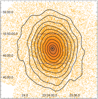
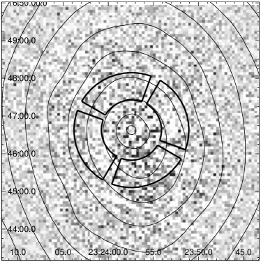
Figure 1.— (Left) MOS1 image in the 0.5-8.0 keV band displayed with logarithmic intensity scaling. This image has not been exposure corrected due to the inaccurate exposure maps available from the standard processing. No additional smoothing has been applied to this image. However, smoothed intensity contours are overlaid to guide the eye. (Right) Residual image of MOS1, displayed with linear intensity scaling, obtained by subtracting from the raw image a model constructed by fitting perfect elliptical isophotes (see text). The region displayed corresponds to the boxed area of the image on the left. The sectors indicate regions analyzed to assess non-ellipsoidal fluctuations as discussed in the text.

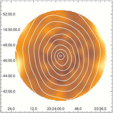
Figure 2.— Hardness ratio image of A2589, displayed with logarithmic intensity scaling, generated using the 0.5-1.3 keV and 1.3-5.0 keV combined MOS1 and MOS2 images (see text for details). Contours represent the X-ray isophotes.

3. Imaging analysis

We display the MOS1 image in Figure 1. The image is not exposure corrected because the standard processing does not provided accurate exposure maps. Since the MOS2 and pn images have more chip gaps and bad columns, we only display the MOS1 image. The diffuse emission is remarkably regularly shaped, being moderately elliptical, and fills the entire field of view. We measure the centroid and the ellipticity of the X-ray surface brightness using the moment method described by Carter & Metcalfe (1980) and implemented in our previous X-ray studies of galaxies and clusters (e.g., Buote & Canizares, 1994). This iterative method is equivalent to computing the (two-dimensional) principal moments of inertia within an elliptical region. The ellipticity is defined by the square root of the ratio of the principal moments, and the position angle is defined by the orientation of the larger principal moment. Following our previous study of the ellipticity of the Chandra data of NGC 720 (Buote et al., 2002) we removed point sources and replaced them with smoothly distributed diffuse emission using the CIAO task dmfilth. Because this method for computing ellipticity cannot account for chip artifacts we restricted the analysis to the central chip on the MOS1.

We defined the following annuli with outer semi-major axes $(a)$ expressed in units of kpc (15, 30, 45, 60, 75, 100, 150, 225). The ellipticity is rather uncertain within $a\sim 30$ kpc because of the small number of pixels (and resolution elements). For $a\gtrsim 60$ kpc the ellipticity falls from near 0.30 to 0.25 at the outer radius with a position angle near $10\arcdeg$ N-E over this entire range.

The intensity weighted center shift, defined similarly to that in Mohr et al. (1995), is $5.4\pm 0.5$ kpc for these annuli. However, the maximum difference between annuli centers is observed between the annulus 45-60 kpc and the central circle (0-15 kpc) where we obtain a difference of 16 kpc in center positions with negligible statistical error. This 45-60 kpc annulus appears to be slightly offset from all of the other annuli. Note that the X-ray peak (R.A.: 23h23h57.4m, DEC: 16d46m38s) coincides precisely with the optical position of the cD galaxy NGC 7647.

The most general non-rotating, self-gravitating equilibrium configuration is the triaxial ellipsoid. The equipotentials of a triaxial ellipsoid are concentric surfaces that themselves are nearly ellipsoids. Since in hydrostatic equilibrium the hot gas traces exactly the same shape as the gravitational potential regardless of the radial temperature profile (Buote & Canizares, 1994, 1996), we expect a relaxed cluster to have concentric isophotes that are nearly elliptical in shape, though the ellipticity may vary with radius. (The position angle of the X-ray isophotes also need not be constant with radius.)

The small center shift we measured above represents a deviation from equilibrium, particularly near the isophotes with $a=45-60$ kpc. We searched for higher order deviations from elliptical symmetry in the following manner. Using the ellipse package within iraf-stsdas we fitted elliptical isophotes to the MOS1 image; we restricted this analysis to the central CCD to avoid complications associated with the chip gaps. Then we constructed a model image from the fitted isophotes and subtracted it from the raw image. The resulting residual image is also displayed in Figure  1. We compared the model image and raw image in 4 sectors defined near the 45-60 kpc annulus; i.e., inner radius 40 kpc, outer radius 75 kpc. For each sector we obtain the following ratios of counts between the raw and model images: North $1.01\pm 0.02$, South $1.04\pm 0.02$, East $0.92\pm 0.02$, West $0.94\pm 0.02$. These values represent quite reasonable scatter about unity considering uncorrected exposure variations. We conclude the image does not show significant deviations from elliptical symmetry apart from the modest center shift noted above.

We also searched for evidence of asymmetry in the temperature (and metallicity) structure using a hardness ratio map. Using the combined MOS1 and MOS2 images we constructed the map as an (S-H)/(S+H) image, where S and H are respectively images in soft (0.5-1.3 keV) and hard (1.3-8.0 keV) bands; the image was then smoothed with a gaussian kernel with width of 1 pixel. We display the hardness-ratio map in Fig. 2. It is quite regular and shows no evidence for significant deviations from elliptical symmetry.

As first reported by David et al. (1996) there is a strong alignment between the optical isophotes of the cD, the X-ray isophotes, and the galaxy isopleths of the host (super-) cluster. It is also worth noting that the average ellipticity of the cluster galaxy isopleths is $\sim 0.3$ (Plionis et al., 1991), consistent with the X-ray isophotes. Beers et al. (1991) reported an offset of the cD velocity ($\sim 250$ km s^-1) from the other member galaxies. However, these sparse data were deemed insufficient to obtain a robust result, and, consequently, this system was not included in the systematic study of cD offsets by Bird (1994). Indeed, the kinematical study by Gebhardt & Beers (1991) using the data of Beers et al. (1991) obtains only weak evidence for substructure.

Evidently, A2589 is nearly in hydrostatic equilibrium. This is indicated by the strong similarity in the distributions of galaxies and ICM, and because A2589 has one of the most regular X-ray images on the $\approx 0.5$ Mpc scale (Buote & Tsai, 1996). The only significant asymmetry we detect is the small center offset associated with the 45-60 kpc annulus mentioned above. We will consider whether this region displays anomalous behavior in our analysis of the azimuthally averaged spectral (and mass) properties below.

Table 1Spectral fit parameters for each annulus

Annulus	$\rm{R_{in}}$	$\rm{R_{out}}$	T	$\rm{Z_{Fe}}$	$\rm{Z_{S}}$	$\rm{Z_{Si}}$	norm	$\rm{\chi^{2}/dof}$	Null Hyp.
	(kpc/arcmin)	(kpc/arcmin)	(keV)	(solar)	(solar)	(solar)	($10^{-3}\rm{cm^{-5}}$)		prob. (%)
1	0/0.00	32/0.65	$3.26\pm 0.08$	$1.33\pm 0.11$	$0.55\pm 0.25$	$1.01\pm 0.20$	$1.38\pm 0.04$	535.3/487	6.39
2	32/0.65	57/1.16	$3.45\pm 0.08$	$0.95\pm 0.07$	$0.17\pm 0.16$	$0.47\pm 0.19$	$2.10\pm 0.04$	654.6/606	8.38
3	57/1.16	93/1.89	$3.61\pm 0.07$	$0.78\pm 0.06$	$<0.22$	$0.30\pm 0.16$	$3.42\pm 0.08$	752.0/730	27.8
4	93/1.89	136/2.76	$3.40\pm 0.05$	$0.77\pm 0.06$	$0.14\pm 0.09$	$0.16\pm 0.08$	$3.72\pm 0.07$	772.9/716	6.91
5	136/2.76	193/3.92	$3.36\pm 0.06$	$0.54\pm 0.05$	$0.22\pm 0.12$	$0.52\pm 0.09$	$3.99\pm 0.06$	653.6/688	82.0
6	193/3.92	289/5.87	$3.52\pm 0.07$	$0.57\pm 0.07$	$<0.12$	$<0.14$	$4.56\pm 0.09$	726.4/676	8.53
7	289/5.87	489/9.93	$3.04\pm 0.15$	$0.43\pm 0.07$	$0.30\pm 0.15$	$0.28\pm 0.19$	$5.40\pm 0.16$	493.5/450	7.12

Note. — Parameters derived by fitting an absorbed apec plasma model to the spectra extracted in each annulus. Columns $Z_{Fe}$, $Z_{S}$, $Z_{Si}$ show the abundance values obtained leaving free to vary Fe, S and Si. The “norm” parameter is the emission measure for the apec code as defined in XSPEC. The last column report the Null Hypothesis Probability for the fit. The total 0.5-8.0 keV luminosity of these annuli is $1.47^{+0.18}_{-0.16}\,10^{43}$ erg s^-1 (90% conf.).

4. Spectral analysis

Since the X-ray image and hardness-ratio map do not display substantial azimuthal variations, we focus our analysis on the X-ray spectral properties derived from circular annuli. We neglect the ellipticity of the X-ray isophotes since determining the flattening of the mass distribution is beyond the scope of this paper. (In any event, using elliptical annuli does not produce qualitatively different profiles of the gas density, temperature, or metallicity when the results are expressed in terms of the mean radius $R=a\sqrt{q}$, where $a$ is the semi-major axis and $q$ is the axial ratio.)

We extracted spectra in the 0.5-8.0 keV energy band from all of the EPIC CCDs in a series of concentric circular annuli centered on the X-ray peak. These annuli were originally constructed to have at least 8000 background-subtracted counts in the MOS1 and were defined to be larger than the XMM PSF and provide temperature constraints of similar precision. Since the central radial bin has the highest S/N, we further divided it into two annuli (each still being larger than the XMM PSF). This allows us to probe the spectral properties down to $\sim 0.015{\hbox{$r_{\rm vir}$}}$. The annuli definitions are listed in Table 1. We do not list results obtained for the outermost annulus ($R>9.93\arcmin$ out to the edge of the fields) that were used in the background determination summarized in §2. At these large radii the source emission contributes little to the EPIC spectra, and thus small changes in our adopted background model translate to relatively large changes in the derived source parameters. (We assess the systematic error resulting from the background level on our mass results in §8.) We also restricted the upper energy limit to 5.0 keV in the penultimate annulus (i.e., the last annulus listed in Table 1) because of excess hard emission that we could not remove with our background model.

In each annulus we fitted a model consisting of an optically thin hot plasma (apec) modified by Galactic absorption. The free parameters are the normalization, temperature, iron, silicon, and sulfur abundances. All other elemental abundances are fixed so that their ratio with respect to iron is solar assuming the abundance standard of Grevesse & Sauval (1998). Error estimates are obtained by simulating spectra based on our best-fitting models. From 20 Monte Carlo simulations we compute the standard deviation of each parameter which we report as the $1\sigma$ error. (All quoted errors are $1\sigma$ unless stated otherwise.)

The results are listed in Table 1 for the model parameters, and we display the MOS1 spectra and best-fitting models for two annuli in Figure 3. The quantities we derive for the hot gas in each annulus are average values weighted by cluster emission projected along the line-of-sight. Below we will obtain the gas density and temperature as a function of three-dimensional radius by projecting models along the line-of-sight and fitting them to the results obtained as a function of projected radius listed in Table 1. We found this procedure to be appropriate given the small number of radial bins and quality of our data. In §8 we also consider the effects on the derived mass profile of first deprojecting the data using the well-known onion-peeling method.

We mention that the generally sub-solar ratios of Si/Fe and S/Fe abundances imply that most of the iron ($\sim 80\%-95\%$) in the hot ICM has been provided by Type Ia supernova, with convective deflagration explosion models favored over delayed-detonation models. These results are consistent with those we have obtained for galaxies and groups (e.g., Buote et al., 2003b; Humphrey & Buote, 2006).

Figure 3.— MOS1 spectra accumulated within (Left Panel) annulus #1 and (Right Panel) annulus #7. Each spectrum is fitted with an apec plasma model modified by Galactic absorption as discussed in §4. Note that these models were fitted simultaneously with the MOS2 and pn data, but we display only the MOS1 for clarity.

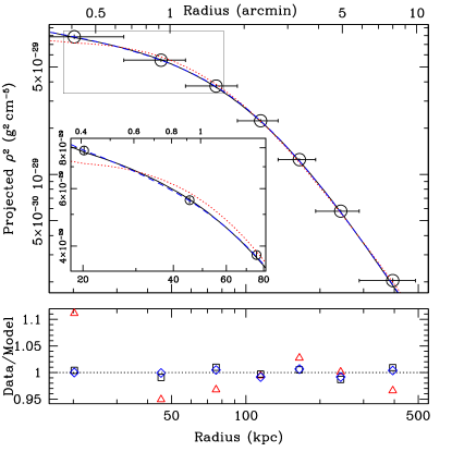
Figure 4.— The radial profile of the projection of $\rho_{g}^{2}$. The data points are proportional to $norm/A$, where $norm$ is listed in Table 1 and $A$ is the area of the annulus. The models have been fitted by weighting the projection integral by the plasma emissivity (see §5). However, for display purposes we do not bin the models in the plot. Because the statistical error bars are very small, we enclose the data points with open circles. Each data point represents a radial bin as defined in Table 1. The horizontal bars represent the width of the annuli. The solid line is the best fit cusp $\beta$ model, the dotted red line is the single $\beta$ model and the dashed blue line is the double $\beta$ model. The cusp $\beta$ model and double $\beta$ model almost entirely overlap. The inset shows an enlarged view of the inner region. In the ratio (data/model) plot, red triangles, blue diamonds and black squares refer respectively to $\beta$ model, double $\beta$ model and cusped $\beta$ model.

5. Gas Density Profile

Table 2Gas Density and Temperature Models

Projected Density			Projected Temperature
$\beta$ model	double $\beta$ model	cusp $\beta$ model	Power-law model	$T(r)^{*}$ model
$\beta\!=\!0.54\pm 0.01$	$\beta\!=0.57\pm 0.02$	$\beta\!=\!0.59\pm 0.02$	$T_{100}\!=\!3.42\pm 0.03\,\rm{keV}$	$A_{1}\!=\!3.6\pm 1.5$
$r_{c}\!=\!76.5\pm 2.4$ kpc	$r_{c1}\!=\!21.9\pm 14.5$ kpc	$r_{c}\!=\!119.2\pm 12.5$ kpc	$\alpha_{p}\!=\!0.0\pm 0.02$	$A_{2}\!=\!3.5\pm 0.9$
$\rho_{g0}=1.40\pm 0.03^{\ast}$	$r_{c2}\!=\!95.2\pm 14.0$ kpc	$\alpha_{c}\!=\!0.38\pm 0.06$	$\cdots$	$r_{p}=100$(fixed)
$\cdots$	$\rho_{g0,1}=2.1\pm 8.0^{\ast}$	$\rho_{g,c}=0.82\pm 0.10^{\ast}$	$\cdots$	$\alpha_{1}=0.21\pm 0.21$
$\cdots$	$\rho_{g0,2}=1.1\pm 0.1^{\ast}$	$\cdots$	$\cdots$	$\alpha_{2}=-0.09\pm 0.15$
$\cdots$	$\cdots$	$\cdots$	$\cdots$	$\gamma=0.45$ (fixed)
$\chi^{2}/dof=27.6/4$	$\chi^{2}/dof=0.67/2$	$\chi^{2}/dof=1.08/3$	$\chi^{2}/dof=21.3/5$	$\chi^{2}/dof=15.0/3$

Note. — Models of the gas density and temperature as a function of three-dimensional radius. The functions and parameters are defined in §5 and §6. The gas density normalizations (^∗) are expressed in units of $10^{-26}$ g cm^-3.

Our analysis of the gravitating mass and dark matter requires that we evaluate derivatives of the gas density and temperature with respect to the three-dimensional radius (§7.1 and §7.3). To reduce the noise in the derivative calculations we fit simple analytic functions to the entire radial range of the gas density and temperature data. For the gas density ($\rho_{g}(r)$) we integrate the quantity, $\rho_{g}^{2}\Lambda(T,\hbox{{$Z_{\rm Fe}$}})$, along the line-of-sight, where $\Lambda(T,\hbox{{$Z_{\rm Fe}$}})$ is just the apec model with $norm=1$. The temperature profile model is fixed to the best-fitting result obtained in the following section. (The iron abundance profile is also fitted with a simple model and extrapolated as a power-law outside the last data point. It also remains fixed during the fit.) The limits of integration are projected radius $R$ and a maximum value, the latter of which we set near 2 Mpc corresponding to the inferred virial radius of the cluster below. (The results are not sensitive to this choice.) Consequently, the integral is obtained as a function of projected radius $R$ which we then evaluate over the radial width of each circular annulus defined in Table 1. The result for each annulus is divided by $\Lambda(T,\hbox{{$Z_{\rm Fe}$}})$, where now $T$ and $Z_{\rm Fe}$ are the emission-weighted results quoted in Table 1 for the annulus in question.

As is standard for such studies, we begin by fitting the gas density profile with the well-known $\beta$ model (Cavaliere & Fusco-Femiano, 1978),

$$\rho_{g}=\rho_{g0}\Big{[}1+\Big{(}\frac{r}{r_{c}}\Big{)}^{2}\Big{]}^{-\frac{3}{2}\beta},$$ (1)

where $\rho_{g0}$ is the central gas density, $r_{c}$ the core radius, and the asymptotic slope is $-3\beta$. The result of fitting this model to the data is shown in Figure 4 and the parameters are listed in Table 2. Although the single $\beta$-model is not formally an acceptable fit, it provides a good representation of the radial profile. The fractional residuals are $<5\%$ in all annuli except the center where a $\sim 10\%$ deviation is observed.

Formally acceptable fits can be obtained by employing conventional modifications of the single $\beta$ model. First, we examine the “cusped $\beta$ model” (Pratt & Arnaud, 2002; Lewis et al., 2003),

$$\rho_{g}=\rho_{g,c}2^{3\beta/2-\alpha_{c}/2}\left(\frac{r}{r_{c}}\right)^{-\alpha_{c}}\left[1+\left(\frac{r}{r_{c}}\right)^{2}\right]^{-\frac{3}{2}\beta+\frac{\alpha_{c}}{2}},$$ (2)

where the exponent $\alpha_{c}$ is the slope of the power-law cusp at small radii and $\rho_{g,c}=\rho_{g}(r_{c})$. Although this model introduces only one additional free parameter over the single $\beta$ model, as is seen in Figure 4 and Table 2 the fit is excellent: residuals at all radii are reduced to $\lesssim 1\%$.

Second, we also investigated adding a second $\beta$ model; i.e., a “double-$\beta$” model (e.g., Xu et al., 1998; Mohr et al., 1999). Even if we require the $\beta$ values of both components to be the same, the fit is excellent – just as good as the cusped $\beta$ model (see Figure 4 and Table 2). Since this model does not improve the fit over the that achieved by cusped $\beta$ model, but it introduces another free parameter, we will use the cusped $\beta$ model as the default profile in the mass analysis below.

The values we obtained for $\beta$ are larger than we obtained previously for A2589 with Chandra data (Buote & Lewis, 2004). Using a single $\beta$ model, which was all that was required by the low-quality ACIS-S observation, we obtained $\beta=0.39\pm 0.04$; i.e., $\approx 4\sigma$ smaller than the result obtained for the single $\beta$ model with the EPIC data. This difference is not surprising since the Chandra data were only fitted out to $\approx 150$ kpc compared to $\approx 500$ kpc in this paper. The $\beta$ values obtained from XMM agree well with the value of 0.57 quoted by David et al. (1996) obtained from ROSAT data.

6. Gas Temperature profile

We display the temperature profile in Figure 5 corresponding to the values in Table 1. The approximately isothermal profile is similar to that measured by Chandra in Buote & Lewis (2004) and does not show the evidence for a cool core indicated by ROSAT (David et al., 1996). The lack of a cool core is unusual for a cluster having such a regular X-ray morphology, though the centrally peaked iron abundance profile is similar to those found in cool core clusters (e.g., De Grandi et al., 2004; Böhringer et al., 2004).

Starting with a model for $T(r)$ we projected the quantities $T\rho_{g}^{2}\Lambda(T,\hbox{{$Z_{\rm Fe}$}})$ and $\rho_{g}^{2}\Lambda(T,\hbox{{$Z_{\rm Fe}$}})$ along the line of sight. (Here we use the best-fitting model for $\rho_{g}(r)$ obtained above, and the $Z_{\rm Fe}$ profile is fixed as before.) These quantities were evaluated within annuli in the same manner as done for the gas density. The projected emission-weighted temperature is obtained by dividing the first term by the second term.

Since the temperature data are nearly isothermal, we initially fitted a single power-law,

$$T(r)=T_{100}\Big{(}\frac{r}{100\,\rm{kpc}}\Big{)}^{\alpha_{p}},$$ (3)

where $T_{100}$ is the temperature at 100 kpc. We show the best-fitting model in Figure 5 and list the parameters in Table 2. The power-law exponent is $\alpha_{p}=0.00\pm 0.02$, indicating an isothermal profile. This result is also consistent with that obtained for the Chandra data by Buote & Lewis (2004); the normalization of the temperature profile obtained from the XMM data is also within $1.2\sigma$ of that obtained from Chandra.

Unlike the low-quality Chandra temperature profile, the XMM temperature data are not formally consistent with the isothermal / power-law model. A better fit can be achieved by adding another degree of freedom to account for the curvature of the profile in the log-log plot. We experimented with several models and adopted a model consisting of two power-laws joined by an exponential cut-off term,

$$T(r)^{*}=T_{1}\,e^{-(\frac{r}{r_{p}})^{\gamma}}+T_{2}\,(1-e^{-(\frac{r}{r_{p}})^{\gamma}}),$$ (4)

where $T_{i=1,2}=A_{i}\Big{(}\frac{r}{r_{p}}\Big{)}^{\alpha_{i}}$ and $A_{i}$, $r_{p}$, $\alpha_{i}$ and $\gamma$ are respectively the normalization, scale radius and slope for the power-laws and the exponent of the power-law functions in the exponentials. This model provides a better fit (Figure 5 and Table 2), though only the fractional residuals of the innermost and outermost data points are affected substantially.

We adopt this profile as our default in our subsequent analysis. In § 8 we assess how different choices of temperature profiles affect our mass measurements. There we also assess the importance of the last data point for determining the best model.

Figure 5.— Projected temperature profile. Open circles represent our XMM observation. The models are emission-weighted projections averaged over each annulus (see §6). However, for display purposes we do not bin the models in the plot. The solid line is the emission weighted $T(r)^{*}$ model. The dashed line is the emission weighted power-law. In the ratio plot the triangles represent the power-law and squares are the $T(r)^{*}$ model.

7. Mass analysis

7.1. Gravitating mass

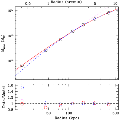
Figure 6.— Gravitating mass profile obtained using the cusp $\beta$ model for the gas density and the $T(r)^{*}$ model for the temperature. The gravitating mass is evaluated at radii corresponding to the annuli used for spectral analysis (§4). We display the best-fitting NFW (solid line), N04 (dashed line) and power-law (only for the three inner data points; dotted line) models.

Table 3Mass profile fit parameters

Profile	$\chi^{2}_{c}\pm\sigma_{\chi^{2}}/dof$	$r_{s}\rm{(kpc)}$	c	$\alpha$	$r_{vir}\rm{(Mpc)}$	$M_{vir}(10^{14}\rm{M_{\odot}})$	$c_{200}$	$M_{200}(10^{14}\rm{M_{\odot}})$
NFW	$12.7\pm 7.3/5$	$286\pm 27$	$6.1\pm 0.3$	$\cdots$	$1.74\pm 0.05$	$3.25\pm 0.29$	$4.6\pm 0.3$	$2.65\pm 0.20$
N04	$\;\;2.4\pm 1.9/4$	$206\pm 21$	$7.0\pm 0.3$	$0.40\pm 0.05$	$1.44\pm 0.08$	$1.84\pm 0.33$	$5.5\pm 0.3$	$1.70\pm 0.24$
Power-law	$\;\;0.2\pm 0.2/1$	$\cdots$	$\cdots$	$1.84\pm 0.18$	$\cdots$	$0.12\pm 0.01$	$\cdots$	$\cdots$

Note. — For the N04 model $r_{s}$ corresponds to $r_{-2}$. For the power-law model $\alpha$ corresponds to $\alpha_{p}$ and the $M_{vir}$ value is the normalization of the model at $100\,\rm{kpc}$. The Power-law model is fitted only to the inner three points.

When hydrostatic equilibrium is a suitable approximation for the hot ICM the gravitating mass ($M_{\rm grav}$) enclosed within a certain radius $r$ can be inferred from the density and temperature of the emitting plasma (Mathews, 1978; Fabricant et al., 1980):

$$M_{\rm grav}(<\!r)=\frac{k_{B}}{G\mu m_{p}}\,rT\left(-\frac{d\ln\rho}{d\ln r}-\frac{d\ln T}{d\ln r}\right),$$ (5)

where $k_{B}$ is the Boltzmann’s constant, $G$ is the constant of gravitation, $\mu$ is the mean atomic weight of the gas (taken to be 0.62), $m_{p}$ is the atomic mass unit. We adopt the cusp $\beta$ model for the gas density and the $T(r)^{*}$ model for the temperature for our fiducial analysis. Using these parameterizations we evaluate the gravitating mass at weighted radii, $r\equiv[(r_{\rm out}^{3/2}+r_{\rm in}^{3/2})/2]^{2/3}$ (see Lewis et al., 2003) within the annuli used for spectral analysis (§4). The resulting mass data points are displayed in Figure 6. The error bars on the data points are the standard deviations derived from the gas density and temperature profiles obtained from each of the 20 Monte Carlo error simulations (§4). Because the mass data points are correlated, it is inappropriate to use the $\chi^{2}$ null-hypothesis probability assuming uncorrelated errors to assess goodness-of-fit. Instead for each mass model we provide the standard deviation of $\chi^{2}$ obtained from fitting a particular mass model (e.g., NFW) to the mass profile obtained for each of the 20 Monte Carlo simulations. This allows one to assess the relative goodness-of-fit between different mass models.

First we examined whether the NFW profile (Navarro et al., 1997) could provide a good description of the mass data. The NFW density profile is given by:

$$\rho(r)=\frac{\rho_{c}(z)\delta_{c}}{(r/r_{s})(1+r/r_{s})^{2}},$$ (6)

where $\rho_{c}(z)$ is the critical density of the universe at redshift $z$, $\delta_{c}$ is a characteristic dimensionless density defined as:

$$\delta_{c}=\frac{1}{3}\frac{\rho_{vir}}{\rho_{c}(z)}\frac{c^{3}}{\ln(1+c)-c/(1+c)},$$ (7)

where $r_{s}$ is the scale radius (the point where the logarithmic slope reaches a value of -2), $\rho_{vir}$ is the mean density of a sphere enclosed in $r_{vir}=cr_{s}$ (where $c$ is the concentration parameter) that is $104.7\rho_{c}(z)$ (see Bryan & Norman, 1998). By integrating equation 6 we obtain the expression of the total mass enclosed within a radius $r$:

$$M_{NFW}(<r)=A_{NFW}\left[\ln(1+r/r_{s})-\frac{r/r_{s}}{1+r/r_{s}}\right],$$ (8)

where $A_{NFW}=4\pi\rho_{c}(z)\delta_{c}r_{s}^{3}$. A distinctive feature of the NFW profile is that the logarithmic slope of the density profile asymptotes to -1 at small radius corresponding to a logarithmic slope in the mass of 2.

We plot the best-fitting NFW model in Fig. 6 (solid line) and list the derived parameters in Table 3. This fit is very good in the sense that the fractional residuals are $<5\%$ for the central radial bin and for $r>100$ kpc. The largest deviation is observed for $r\sim 50$ kpc where the fractional residual is $\sim 13\%$. It is interesting that this radius corresponds to the largest center shift in the X-ray isophotes (§3). The values of $c$ and $M_{\rm vir}$ obtained for the NFW fit are very consistent with those obtained from recent observations of relaxed clusters with Chandra and XMM (e.g., Lewis et al., 2003; Pointecouteau et al., 2005; Vikhlinin et al., 2006). (These results are also consistent with those we obtained previously from the low-quality Chandra AO-3 data.) These $c$ and $M_{\rm vir}$ values agree extremely well with the mean relation predicted by the $\Lambda$CDM simulations of Bullock et al. (2001), where we have extended their toy model up to virial masses appropriate for A2589.

To obtain an estimate of the slope of the inner density profile without reference to the NFW model we fitted the three inner mass data points with a power-law (see Eq. 3; thin dotted line in the plot). The value we obtain is $1.84\pm 0.18$ for the mass which corresponds to $-0.84\pm 0.18$ for the density. This value is consistent with the inner logarithmic slope given by an NFW profile within the $1\sigma$ error. The inner slope of -0.8 is also consistent with a direct solution of the radial Jeans equation for DM assuming an isotropic velocity dispersion tensor and a CDM phase-space density (Hansen & Stadel, 2005).

Finally, we also examined the Sersic-like profile (Navarro et al., 2004, hereafter N04) that was recently suggested as a better parametrization for CDM halos, particularly within the very inner regions (less then few percent of the virial radius) where it is typically shallower than NFW (see also Graham & et al., 2005). The N04 density profile is defined as follows,

$$\rho(r)=\rho_{-2}\,\rm{exp\left({\frac{2}{\alpha}}\right)exp\left[{-\frac{2}{\alpha}x^{\alpha}}\right]},$$ (9)

where $x=r/r_{\rm{-2}}$, and the quantities flagged with -2 refer to the point where the profile reaches a logarithmic slope of -2 ($r_{\rm{-2}}$ is the analog of $r_{s}$ in the NFW profile). The $\alpha$ exponent determines the bend of the profile about $r_{\rm{-2}}$. The enclosed mass obtained by integrating this expression is:

$$M_{N04}(<r)=A_{N04}\,\frac{1}{\alpha}\,\rm{exp\bigg{(}\frac{2}{\alpha}\bigg{)}}\bigg{(}\frac{\alpha}{2}\bigg{)}^{3/\alpha}\gamma\bigg{(}\frac{3}{\alpha},\frac{2}{\alpha}x^{\alpha}\bigg{)},$$ (10)

where $A_{N04}=4\pi\rho_{-2}r_{-2}^{3}$ and $\gamma(\eta,\lambda)=\int_{0}^{\lambda}t^{\eta-1}e^{-t}dt$ is the lower incomplete gamma function.

We display the best-fitting N04 profile in Figure 6 represented by a dashed line. The fractional residuals are smaller than the NFW profile at all radii except the central data point where the residual is about 50%. The smaller $\chi^{2}$ value obtained for the N04 arises primarily from the better fit of the data point $r\sim 50$ kpc. The inferred value of $\alpha=0.40\pm 0.05$ is quite large and incompatible with the mean value of $0.172\pm 0.032$ for CDM halos (Navarro et al., 2004). Consequently, the result we obtain for the concentration and virial mass using the N04 model must be interpreted with caution; i.e., the large $\alpha$ implies a density profile that is shallower in the center and steeper at large radii than CDM.

Using our measurement of the gravitating mass obtained from the NFW model and the gas mass obtained by integrating the cusp $\beta$ model we compute the gas fraction as a function of radius. For the central data point we obtain $f_{gas}=0.014\pm 0.004$ while it rises to $0.083\pm 0.002$ for our outermost mass data point. This value is consistent with values obtained by Sanderson et al. (2003) and Vikhlinin et al. (2005) for clusters of similar temperature. If we extrapolate our fits to the virial radius we obtain a total gas fraction $f_{gas}=0.168\pm 0.009$, consistent with the value of the baryon fraction $\Omega_{b}/\Omega_{m}\sim 0.17$ measured by WMAP (Spergel et al., 2003).

7.2. The Ratio of Gravitating Mass to cD Stellar Light

The radial profile of the ratio of gravitating mass to stellar light in the cluster provides a useful diagnostic for the radius where dark matter dominates the cluster mass budget. We shall only consider the optical light of the cD galaxy NGC 7647 since only sparse information in the literature exists for a small number of other member galaxies. Fortunately, the $V$-band surface brightness profile of the cD galaxy has been analyzed by Malumuth & Kirshner (1985) out to a radius of $\sim 130\,\rm{kpc}$. They find that a King model is a good fit to the optical data with a core radius, $r_{c}=0.98\,\rm{h_{70}^{-1}kpc}$, and a total $V$-band luminosity $L_{V}=2.3\times 10^{11}\,\rm{L_{V,\odot}}$ within the region analyzed. They find that a de Vaucouleurs model with $r_{e}=32.6$ kpc fits the optical data nearly as well. Therefore, we represent $L_{V}(r)$ by a Hernquist model (Hernquist, 1990) with scale radius $a=r_{e}/1.8153=18.0$ kpc and total luminosity quoted above, since the projected Hernquist profile is a good approximation to a de Vaucouleurs profile.

In Fig. 7 we plot $M_{grav}(<\!r)/L_{V}(<\!r)$: the ratio of gravitating mass, computed using the NFW model, to the integrated V-band luminosity of the cD, using the Hernquist model, as a function of radius. The $M_{grav}/L_{V}$ profile increases from $9.0\pm 2.3\,\rm{M_{\odot}/L_{V,\odot}}$ for the inner data point to $93.5\pm 2.3\,\rm{M_{\odot}/L_{V,\odot}}$ at the radius representing the outer extent of the optical data. If we extrapolate the Hernquist model of the cD out to the extent of the X-ray measurements, $M_{grav}/L_{V}$ increases to $433\pm 9\,\rm{M_{\odot}/L_{V,\odot}}$ (gray area in Fig. 7). This latter value is an upper limit to the cluster mass to light ratio because we have not considered additional contributions from other member galaxies.

There is no evidence that the $M_{\rm grav}/L_{V}$ profile flattens at small radius such as we have observed for A2029 (Lewis et al., 2003) and for a sample of early-type galaxies (Humphrey et al., 2006). Since the flattening in the profiles in other systems occurs for $r\lesssim 10$ kpc, yet our central bin has outer radius $r=32$ kpc, we do not expect to detect this effect. High quality Chandra data would allow $M_{\rm grav}/L_{V}$ to be probed on the small scales necessary for an interesting comparison to other systems.

We mention that Malumuth & Kirshner (1985) used their fit of the King model and a measurement of the central velocity dispersion to estimate $M_{\rm grav}/L_{V}$ at the very center; i.e., within the King core radius ($<1$ kpc). They obtain $M_{grav}/L_{V}\approx 15$ in solar units, converting their value to our redshift and cosmology. This value is a factor of 1.7 larger than we have measured at $r\sim 20$ kpc, although the discrepancy is not highly significant ($2.6\sigma$). For a single burst stellar population with age ranging from 10-13 Gyr and metallicity ranging from 0.5-2 solar the $V$-band stellar mass-to-light ratio is only expected to take values from 5-10 in solar units, with values at the upper end assuming a Salpeter IMF. (We have used the results of Maraston 1998 from updated model grids provided by the author.) The gravitating mass we measure for $r\sim 20$ kpc is similar to that we have measured at that radius in the cluster A2029 and a sample of elliptical galaxies (Lewis et al., 2003; Humphrey et al., 2006). If the difference in masses estimated from the X-ray and optical methods is real, it likely implies the stellar mass-to-light ratio in the cD varies with radius.

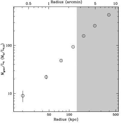
Figure 7.— Ratio of the total gravitating mass to the optical light of the cD galaxy. The data in the gray area are estimated from an extrapolation of the Hernquist profile approximation of the De Vaucouleurs profile obtained by Malumuth & Kirshner (1985) to map the V-band light profile out to $\sim 130\,\rm{kpc}$.

7.3. Dark matter

We desire to extract the radial profile of the DM from the gravitating matter by removing the contributions of the known luminous mass components. Since the X-ray data provide a direct measurement of the hot gas density, it is straightforward to compute the radial profile of $M_{\rm grav}-M_{\rm gas}$. Consequently, as a first step we fitted single-component models to this “DM” profile analogously to our procedure in the previous section.

The fitted parameters for the NFW, N04, and power-law models are listed in Table 4. Since the hot gas contributes $<10\%$ to the total mass over the radial range fitted, it is not surprising that the parameters we infer are very consistent with those obtained when fitting the total gravitating matter (Table 3). However, we emphasize that $r_{\rm vir}$ and $M_{\rm vir}$ (and hence $c$) obtained in this way refer only to the DM component. To obtain the true values that include the mass of the hot gas we add $M_{\rm gas}$ to $M_{\rm DM}$, compute a new $r_{\rm vir}$, and iterate. For the NFW model this yields ${\hbox{$r_{\rm vir}$}}=1.77\pm 0.04$ Mpc, ${\hbox{$M_{\rm vir}$}}=3.46\pm 0.26\,\times 10^{14}\hbox{{$M_{\odot}$}}$, $c=6.8\pm 0.4$, and a total gas fraction, $f_{g}=0.16\pm 0.01$. It should be remembered that these re-scaled values depend on the extrapolation of our model for $\rho_{g}$ out to $r_{\rm vir}$.

Next we attempted to better isolate the DM profile by removing the contribution of the mass from the stars in the cD. To model the cD stars we employed the Hernquist parameterization of the $V$-band luminosity described in the previous section, which we now refer to as the H90 model. We fitted two-component models, DM + stars, to the radial profile of $M_{\rm grav}-M_{\rm gas}$, where the total mass in the stars is specified by the stellar mass-to-light ratio, ${M_{*}/L_{V}}$.

The results of the fits are listed in Table 4. If ${M_{*}/L_{V}}$ is allowed to be a free parameter in the NFW+H90 fit, then an unphysically small value ${M_{*}/L_{V}}\sim 0.15$ (solar units) is obtained. The NFW model itself is all that is required to describe the mass profile; adding in a separate stellar component only degrades the fit.

We desired to explore the importance of adiabatic contraction of the DM halo arising from the early condensation of baryons in the central galaxy (e.g., Blumenthal et al., 1986; Gnedin et al., 2004). We refer to the modified NFW fit as “NFW*AC+H90”, indicating that adiabatic contraction only applies to the DM component. Because the fitted ${M_{*}/L_{V}}$ is so small, the AC model does not have a substantial effect when ${M_{*}/L_{V}}$ is allowed to be a free parameter. Consequently, we also tried fixing ${M_{*}/L_{V}}=9.0$ (solar units) corresponding to the gravitating mass-to-light ratio obtained for our inner data point, as well as being a reasonable estimate from stellar population synthesis models, as discussed in the previous section. With this ${M_{*}/L_{V}}$ the NFW+H90 and NFW*AC+H90 fits are quite poor within $r\sim 50$ kpc, and the effect of adiabatic contraction on the derived parameters for the DM is roughly equal to that arising from adding the stellar component; e.g., $c$ changes from 6.3 (NFW) to 5.2 (NFW+H90) and from 5.2 (NFW+H90) to 4.3 (NFW*AC+H90). The adiabatic contraction of the dark matter produces a more centrally concentrated halo that deviates even more strongly with the data within $r\sim 50$ kpc (see Figure  8).

Since the N04 model fitted to the total gravitating matter in §7.1 underestimates the mass at the center, it is expected that, unlike the NFW profile, it will allow for a substantial contribution from a central stellar mass component. Indeed, the N04+H90 fit yields a stellar mass-to-light ratio, ${M_{*}/L_{V}}=4.8\pm 1.9$, which is consistent with expectations of single-burst stellar populations synthesis models. Applying adiabatic contraction (i.e., N04*AC+H90) yields a smaller, though still reasonable, value, ${M_{*}/L_{V}}=3.1\pm 0.7$. However, the values of $\alpha\sim 0.5$ obtained for these models, even larger than obtained for the fit to the gravitating matter, are even more inconsistent with the values of $\sim 0.20$ required to represent CDM halos (Navarro et al., 2004). Also, exactly as for the total gravitating matter, it is the data point near $r\sim 50$ kpc that is largely responsible for the better fit of the high-$\alpha$ N04 model with respect to NFW (see Figure  8).

Table 4Model Fits to $M_{\rm grav}-M_{\rm gas}$

Single-Component Models: Dark Matter Only
Model	$M_{*}/L_{V}$	$\chi^{2}_{c}\pm\sigma_{\chi^{2}}/dof$	$r_{s}\rm{(kpc)}$	c	$\alpha$	$r_{vir}\rm{(Mpc)}$	$M_{vir}(10^{14}\rm{M_{\odot}})$
NFW	$\cdots$	$12.4\pm 7.1/5$	$264\pm 26$	$6.3\pm 0.4$	$\cdots$	$1.65\pm 0.05$	$2.78\pm 0.25$
N04	$\cdots$	$\;\;2.4\pm 1.9/4$	$193\pm 19$	$7.1\pm 0.3$	$0.41\pm 0.07$	$1.37\pm 0.08$	$1.58\pm 0.28$
Power-Law	$\cdots$	$\;\;0.2\pm 0.2/1$	$\cdots$	$\cdots$	$1.82\pm 0.18$	$\cdots$	$0.11\pm 0.01$
Two-Component Models: Dark Matter + cD Stars
Model	$M_{*}/L_{V}$	$\chi^{2}_{c}\pm\sigma_{\chi^{2}}/dof$	$r_{s}\rm{(kpc)}$	c	$\alpha$	$r_{vir}\rm{(Mpc)}$	$M_{vir}(10^{14}\rm{M_{\odot}})$
NFW+H90	$(9)$	$42.0\pm 18.0/5$	$338\pm 21$	$5.2\pm 0.3$	$\cdots$	$1.74\pm 0.05$	$3.26\pm 0.29$
NFW+H90	$0.15\pm 0.02$	$12.7\pm 7.1/5$	$263\pm 16$	$6.2\pm 0.3$	$\cdots$	$1.65\pm 0.05$	$2.78\pm 0.25$
NFW*AC+H90	$(9)$	$76.9\pm 25.2/5$	$428\pm 32$	$4.3\pm 0.3$	$\cdots$	$1.84\pm 0.07$	$3.84\pm 0.45$
NFW*AC+H90	$0.055\pm 0.001$	$12.6\pm 7.2/4$	$264\pm 18$	$6.2\pm 0.4$	$\cdots$	$1.65\pm 0.05$	$2.78\pm 0.25$
N04+H90	$(9)$	$\;\;2.0\pm 4.2/4$	$\!\!190\pm\;6$	$6.6\pm 0.1$	$0.61\pm 0.05$	$1.25\pm 0.03$	$1.20\pm 0.09$
N04+H90	$4.8\pm 1.9$	$\;\;0.7\pm 0.7/3$	$\!\!190\pm\;9$	$6.8\pm 0.2$	$0.51\pm 0.05$	$1.30\pm 0.04$	$1.34\pm 0.12$
N04*AC+H90	$(9)$	$\;8.2\pm 7.1/4$	$\!\!195\pm\;6$	$6.1\pm 0.1$	$0.81\pm 0.08$	$1.20\pm 0.03$	$1.04\pm 0.07$
N04*AC+H90	$3.1\pm 0.7$	$\;0.8\pm 1.1/3$	$\!\!191\pm\;7$	$6.8\pm 0.1$	$0.53\pm 0.06$	$1.29\pm 0.04$	$1.32\pm 0.13$

Note. — For the power-law model $M_{vir}$ is the value of the normalization at $100\,\rm{kpc}$. Fixed parameters are enclosed in parenthesis. “*AC” indicates the dark matter component is compressed adiabatically following the prescription of Gnedin et al. (2004). Note that the virial radii and mass refer only to the dark matter component.

Figure 8.— Models fitted to $M_{\rm grav}-M_{\rm gas}$. (left panel) The solid line represents the pure NFW profile, the dashed line adds the stellar component (NFW+H90) with $M_{*}/L_{V}=9.0$ in solar units, and the dotted line applies adiabatic contraction to the NFW profile (NFW*AC+H90) with $M_{*}/L_{V}=9.0$. (right panel) Same as left panel except the NFW profile is replaced with the N04 profile.

Table 5Estimation of the systematic errors

NFW*AC+H90
Parameter	$\rm{Bestfit}$	$\Delta_{stat}$	$\Delta_{bkgmod}$	$\Delta_{bndwidt}$	$\Delta_{mod}(T/\rho)$	$\Delta_{exclpts}($1 - 6$/$2 - 7$)$	$\Delta_{cen}$	$\Delta_{deproj}$
c	$6.2$	$\pm 0.4$	$+0.4\pm 0.4$	$-0.7$	$+0.6\pm 0.6/-1.0$	$-0.6/+0.6$	$\cdots$	$-2.4$
$M_{vir}$	$2.78$	$\pm 0.25$	$\cdots$	$+0.71$	$-0.30/+1.22$	$+0.92/-0.36$	$\cdots$	$+4.11$
$M_{*}/L_{V}$	$0.055$	$\pm 0.001$	$-0.054$	$-0.051$	$-0.044/-0.041$	$-0.045/-0.043$	$-0.044$	$-0.025$
N04*AC+H90
Parameter	$\rm{Bestfit}$	$\Delta_{stat}$	$\Delta_{bkgmod}$	$\Delta_{bndwidt}$	$\Delta_{mod}(T/\rho)$	$\Delta_{exclpts}($1 - 6$/$2 - 7$)$	$\Delta_{cen}$	$\Delta_{deproj}$
c	$6.8$	$\pm 0.1$	$+0.5$	$\cdots$	$\pm 0.6/-0.4$	$+0.3/+0.5$	$-0.3$	$-1.0$
$M_{vir}$	$1.32$	$\pm 0.13$	$-0.21$	$\cdots$	$+0.16/-0.10$	$-0.50/+0.16\pm 0.38$	$\cdots$	$\cdots$
$\alpha$	$0.53$	$\pm 0.06$	$+0.07\pm 0.05$	$\cdots$	$-0.14/+0.34$	$+0.26/-0.13$	$\cdots$	$+0.33$
$M_{*}/L_{V}$	$3.1$	$\pm 0.7$	$-2.4$	$-0.8\pm 1.1$	$(-3.1,+4.0)/+2.5$	$+1.5\pm 1.2/-3.1$	$+2.1$	$+3.3\pm 2.2$

Note. — $\Delta_{stat}$ is the $1\sigma$ statistical error estimate. $M_{vir}$ is expressed in units of $10^{14}\,\rm{M_{\odot}}$.

8. Assessment of systematic errors in the mass profile derivation

In this section we provide estimates of the magnitude of systematic errors on the parameters parameters we have deduced for the dark matter. We illustrate the effects of systematic errors on two fiducial two-component models consisting of a stellar component and adiabatically compressed dark matter: NFW*AC+H90 and N04*AC+H90. The results are summarized in Table 5. The statistical error of the default model ($\Delta_{stat}$) is also listed in the table. For each variant model involved in the systematic checks, we also obtain a corresponding statistical error ($\Delta_{sys}$). If $\Delta_{sys}>=\Delta_{stat}$ we also quote its magnitude with the associated best-fitting parameter shift in the table. For example, the concentration parameter for the NFW*AC+H90 model has a shift of $0.4\pm 0.4$ in the $\Delta_{bkgmod}$ column; i.e., $\Delta_{sys}=\Delta_{stat}$ in this case. We emphasize that none of the systematic checks that we explored can increase the inferred $M_{*}/L_{V}$ for the NFW*AC+H90 model to values 5-10 expected from the stellar population.

In the following we describe the different checks performed:

1. PSF: As stated in §4 we defined our annuli to have at least a width of $1\arcmin$; in particular the central radial bin is a circle of radius $30\arcsec$. With this choice the central circle encloses about 90% of the energy of a point source. Furthermore, since the radial temperature profile is observed to be nearly isothermal we expect that our measured “spectroscopic” temperature should differ negligibly from the emission-weighted temperature within the bin (e.g., Mazzotta et al., 2004). The consistency of our results with those obtained from the lower S/N, but higher resolution, Chandra data (§5 and 6), and with XMM and Chandra observations of other clusters (see below in §10), suggests that the larger XMM PSF has not biased our derived density and temperature parameters by amounts more than the estimated statistical errors.

2. Background modeling ($\Delta_{bkgmod}$ in Table 5): the major sources of uncertainty in the background modeling are the shape of the broken power-law that takes into account the instrumental background at high energies and the level of the CXB component. We assess the influence of these contributions by a variation of $\pm 20\%$ in the slope of the high energy part of the broken power-law and in the normalization of the CXB component. We also set the parameters of the broken power-law to the values obtained fitting the spectrum of the out of field of view events. This last check almost always produced the major source of uncertainty, especially because it caused the outermost data point to vary appreciably. However, this check does not produce results that differ appreciably from the best fit value except for the mass to light ratio inferred for the N04*AC+H90 profile.

3. We varied the band-width in which the spectrum in each annulus has been fitted ($\Delta_{bndwidt}$ in Table 5). We choose to restrict our analysis to the 0.5-5 keV and 1-5 keV bands. Only the NFW profile is affected by this check.

4. We tried different models for the temperature and density profiles (that are shown separately in $\Delta_{mod}$ in Table 5). The models we used are three for the temperature (the first three presented below) and one for the density. They are:

   1. the power-law presented in Eq. 3;

   2. a lognormal profile;

   3. a profile that joins smoothly two power-laws: $T(r)=(P_{1}^{\beta_{1}}+P_{2}^{\beta_{2}})^{-1/\sigma}$, where $P_{1}$ and $P_{2}$ are the power-laws (Eq. 3);

   4. a double $\beta$ model with the $\beta$’s tied.

   It is worth noting that for both the DM parameterizations the lognormal profile gives results very similar to the best fit. For the N04*AC+H90 parametrization the third profile does not allow for the presence of any central stellar component and the power-law temperature model predict a very high M/L. The different density parametrization has a noticeable impact on the NFW profile.

5. We tried to exclude from the analysis either the first or the last annulus ($\Delta_{exclpts}$ in Table 5). We excluded them either only during the fitting of the dark matter profile or also in the temperature and density fitting. We show them separately in Table 5 as 1-6 (last point excluded) and 2-7 (first point excluded). These points influence critically either the form of the dark matter profile (case 1-6) or the dominance of the central stellar component (case 2-7).

6. We repeated the analysis using annuli centered on the X-ray centroid of the cluster ($\Delta_{cent}$ in Table 5). The parameters did not change much and their differences from the best fit values are smaller than the statistical errors.

7. We analyzed the effect of the deprojection on the data ($\Delta_{deproj}$ in Table 5) using the “onion-peeling” technique (e.g. Buote, 2000; Buote et al., 2003a). The quality of the current data does not allow good constraints with this technique.

9. Non-Thermal Pressure Support

Our analysis of the mass profile of A2589 inferred from the XMM data indicates that the NFW model provides a good description of the total gravitating mass profile. However, it is widely thought that the central dark matter profile will be compressed adiabatically because the stellar baryons would have collapsed at early times (e.g., Blumenthal et al., 1986; Gnedin et al., 2004). As we have shown in §7.3 the adiabatic contraction model assuming a reasonable stellar mass-to-light ratio for the cD galaxy exceeds the mass data in the central $r\lesssim 50$ kpc.

We investigate whether plausible additional pressure support from non-thermal processes could reconcile the XMM mass profile with the adiabatic contraction scenario. Since the most important non-thermal pressure should arise from turbulent motions and magnetic fields in the hot ICM, we shall focus our attention on them. We do not consider possible pressure support from cosmic rays which, in principle, could be of the same magnitude as that arising from magnetic fields. As pointed out by Loeb & Mao (1994), the fact that S-Z measurements of clusters are not dominated by a synchrotron signal, the pressure from cosmic ray electrons should be much less than the thermal pressure in clusters. However, the pressure from cosmic ray protons may still be important.

For simplicity we follow Loeb & Mao (1994) and assume,

$$P_{\rm nontherm}=\alpha P_{\rm therm},$$ (11)

where $\alpha$ is a constant. This expression cannot be strictly valid since we expect little contribution from non-thermal pressure for $r\gtrsim 100$ kpc. For our purposes we require only that $d\alpha/dr$ can be neglected at the radii of interest. If we also assume that the equation of hydrostatic equilibrium remains a good approximation but with the thermal gas pressure, $P_{\rm therm}$, replaced by the total pressure, $P_{\rm nontherm}+P_{\rm therm}$, then we have at any radius $r$,

$$\alpha=\frac{M(<r)_{\rm NFW*AC+H90}}{M(<r)_{\rm NFW}}-1,$$ (12)

where $M(<r)_{\rm NFW}$ is the mass determined from fitting the NFW model to the total gravitating matter (Table 3), and $M(<r)_{\rm NFW*AC+H90}$ is the mass obtained from the adiabatically contracted NFW model assuming ${M_{*}/L_{V}}=9.0$ in solar units for the cD galaxy (Table 4).

For our inner mass data point ($r=20.2$ kpc), where the discrepancy is largest (see Figure 8), we obtain $\alpha=0.93$ using our best-fitting models. Note that the NFW*AC+H90 value is $\approx 4\sigma$ larger than the mass data point. For the second mass data point, $r=45.3$ kpc, we obtain a smaller value, $\alpha=0.27$, though the NFW*AC+H90 mass value remains $\approx 4\sigma$ larger than the mass data point. (Note that the NFW mass value is only $1.5\sigma$ larger than the second mass data point.)

9.1. Turbulence

If we assume that the only source of non-thermal pressure arises from random (isotropic) turbulent motions, $P_{\rm turb}=\frac{1}{3}\rho_{g}\langle v^{2}_{\rm turb}\rangle$, then equations (11) and (12) imply,

$$v_{\rm turb}=\sqrt{\alpha}\left(\frac{k_{B}T}{3.26\,\rm keV}\right)^{0.5}\,\rm 1233\,km\,s^{-1},$$ (13)

where the gas temperature corresponding to the inner radial bin (Table 1) has been used. For our inner mass data point ($r=20.2$ kpc) this gives, $v_{\rm turb}\approx 1.3c_{s}$, where $c_{s}=919$ km/s is the adiabatic thermal sound speed of the gas. The generally undisturbed appearance of this cluster (§3) argues strongly against a turbulent velocity this large. For the second mass data point, $r=45.3$ kpc, we also have a very large velocity, $v_{\rm turb}\approx 0.7c_{s}$, where $c_{s}=945$ km/s corresponding to $k_{B}T=3.45$ keV. Cosmological simulations generally find much smaller levels of turbulence in cluster cores, $v_{\rm turb}=0.1-0.3\,c_{s}$ (e.g., Nagai et al., 2003; Faltenbacher et al., 2005). In fact, for lower mass clusters like A2589, Dolag et al. (2005) conclude that only $\approx 5\%$ of the total pressure can be ascribed to turbulent motions.

A further check on the viability of turbulent pressure support is to verify whether, $l$, the eddy size corresponding to $v_{\rm turb}$, is smaller than the length scale under consideration. In an approximate steady state the energy produced by turbulent motions must be dissipated on appropriate viscous length scales or else the gas will be rapidly heated. After setting the rate of turbulent energy generation equal to the rate of radiation energy loss, we solve for the eddy size,

$$l = \alpha^{1.5}\left(\frac{k_{B}T}{3.26\,\rm keV}\right)^{1.5}\left(\frac{\rho_{g}}{2.6\times 10^{-26}\,\rm g\,cm^{-3}}\right)^{-1}\times$$ (14)

$$\left(\frac{\Lambda(T,Z)}{1.7\times 10^{-23}\,\rm erg\,cm^{3}\,s^{-1}}\right)^{-1}\,\rm 3.2\,Mpc,$$

where $\rho_{g}$ is the gas density at $r=20.2$ kpc and $\Lambda(T,Z)$ is the plasma emissivity evaluated for the conditions of the inner annulus (Table 1). The eddy size is vastly larger than the $r\sim 20$ kpc scale of the central region under consideration – and is even larger than the virial radius of $\sim 1.7$ Mpc. We conclude that pressure arising from random turbulent motions in the core cannot reconcile our measurement with the NFW*AC+H90 model.

9.2. Magnetic Fields

Now taking magnetic fields to supply all of the necessary non-thermal pressure ($B^{2}/8\pi$), we obtain from equations (11) and (12),

$$B=\sqrt{\alpha}\left(\frac{k_{B}T}{3.26\,\rm keV}\,\frac{\rho_{g}}{2.6\times 10^{-26}\,\rm g\,cm^{-3}}\right)^{0.5}\,\rm 58\,\mu G,$$ (15)

where, as above, we have taken $T$ and $\rho_{g}$ appropriate for our inner mass data point, $r=20.2$ kpc. For $\alpha=0.93$ the required magnetic field for the inner mass data point is, $B=56\mu$G. Fields of similar magnitude have been suggested previously to explain X-ray mass discrepancies using ROSAT and Einstein data within the central $<1$ kpc of the disturbed elliptical galaxy NGC 4636 (Brighenti & Mathews, 1997). A field strength of $53\mu$G was also suggested previously by Loeb & Mao (1994) to explain the discrepancy between X-ray and lensing mass estimates in the core of the cluster A2218.

But the typical magnetic fields in galaxy clusters range from $1-10\mu$G, much lower than required for interesting pressure support (e.g., for a review see Govoni & Feretti, 2004). Larger fields have been measured in some clusters with strong radio sources. A particularly interesting case is A2029, which, though more massive, appears to be very relaxed both within the core and on larger scales like A2589 (Lewis et al., 2002). Unlike the radio-quiet A2589, the cluster A2029 possesses a Wide-Angle-Tail radio source from which Eilek & Owen (2002) estimate a field of $16\mu$G within 8 kpc of the center of A2029. This field does not provide interesting pressure support, and the strength likely declines rapidly with increasing radius (Govoni et al., 2001).

Although we recognize that there remain outstanding issues in the determinations of magnetic fields in clusters, current evidence clearly does not favor field strengths of $\approx 56\mu$G in galaxy clusters. Therefore, we believe that magnetic pressure support is an unlikely explanation to reconcile the NFW*AC+H90 model with the XMM mass data we have presented for A2589.

10. Conclusions

Using a new XMM observation we have presented an analysis of the radial mass profile inferred from the properties of the hot ICM of the radio-quiet galaxy cluster A2589. We have confirmed the highly regular X-ray image morphology indicated by previous X-ray observations possessing lower resolution and/or lower S/N (David et al., 1996; Buote & Lewis, 2004). The only notable deviation of the X-ray image from concentric ellipses is a $\approx 16$ kpc shift of the X-ray center of the $R=45-60$ kpc annulus. The radial temperature profile is nearly isothermal unlike most X-ray regular clusters which display cool cores (e.g., De Grandi & Molendi, 2002). However, the metallicity does peak at a value near solar at the center and falls off with increasing radius similar to that in cool-core clusters (e.g., De Grandi et al., 2004; Böhringer et al., 2004). Overall, given the highly regular nature of the X-ray image and spectral properties, and the fact it is bright, nearby, and possess no significant radio emission from the central galaxy, A2589 is an especially good target for X-ray studies of its mass distribution.

We find that the NFW profile fits the total gravitating matter ($M_{\rm grav}$) very well over the region studied ($r=0.015-0.25\,\rm{r_{vir}}$, fractional residuals $\lesssim 10\%$) with $c_{\rm vir}=6.1\pm 0.3$ and $M_{\rm vir}=3.3\pm 0.3\times 10^{14}M_{\odot}$ ($r_{vir}=1.74\pm 0.05$ Mpc) in excellent agreement with the $\Lambda$CDM prediction (Bullock et al., 2001). However, if we attempt to add a component to the mass profile representing the stellar mass of the cD galaxy with a reasonable stellar mass-to-light ratio, the fit is degraded substantially in the central $\sim 50$ kpc. Modifying the dark matter halo as the result of adiabatic contraction arising from the early condensation of stellar baryons in the cD (e.g., Blumenthal et al., 1986; Gnedin et al., 2004) further degrades the fit.

If instead we use the Sersic-like profile proposed by Navarro et al. (2004) to represent CDM halos, then sizable stellar mass-to-light ratios are implied that are reasonably consistent with predictions from single burst stellar population models. However, the inverse Sersic index, $\alpha\sim 0.5$, obtained from the fits is a factor of $\sim 3$ higher than predicted; the dark matter profile in the core is inferred to be shallower than CDM. Hence, we are unable to obtain a good fit with a model consisting of CDM halo and a separate contribution from the stars in the cD galaxy with a reasonable stellar mass-to-light ratio.

The good fit of the NFW profile to the total gravitating matter of regular galaxy clusters appears to be a common feature of X-ray studies. The bright, highly relaxed cluster A2029 follows the NFW profile all the way down to $\approx 0.001{\hbox{$r_{\rm vir}$}}$ (Lewis et al., 2003). Dedicated studies of small samples of other mostly relaxed clusters with Chandra and XMM (Pointecouteau et al., 2005; Vikhlinin et al., 2006) also do not report significant deviations from the NFW profile arising from central stellar mass, except for some lower mass, group-scale objects (Vikhlinin et al., 2006; Gastaldello et al., 2006).

Since it seems unlikely that deviations from hydrostatic equilibrium in the hot ICM have conspired in the same way in all of these (regular) clusters to produce a mass profile consistent with NFW in the center, we conclude that the adiabatic contraction scenario does not appear to describe the formation of X-ray clusters. In particular, for A2589 we have estimated the amount of non-thermal pressure support in the hot ICM from random turbulent motions and magnetic fields and conclude that neither source, especially turbulence, can reconcile the XMM mass profile with the adiabatic contraction scenario assuming a reasonable stellar mass-to-light ratio in the cD. We suggest that X-ray observations of A2589 and other relaxed clusters favor the scenario where processes during halo formation, such as the heating of the dark matter by dynamical friction with member galaxies, counteracts adiabatic compression and leads to a total gravitating mass profile consistent with the pure NFW profile (e.g., El-Zant et al. 2004; see also Loeb & Peebles 2003).

References

- Arnaud (2005) Arnaud, M. 2005, astro-ph/0508159
- Bîrzan et al. (2004) Bîrzan, L., Rafferty, D. A., McNamara, B. R., Wise, M. W., & Nulsen, P. E. J. 2004, ApJ, 607, 800
- Böhringer et al. (2004) Böhringer, H., Matsushita, K., Churazov, E., Finoguenov, A., & Ikebe, Y. 2004, A&A, 416, L21
- Barcons et al. (2000) Barcons, X., Mateos, S., & Ceballos, M. T. 2000, MNRAS, 316, L13
- Beers et al. (1991) Beers, T. C., Gebhardt, K., Forman, W., Huchra, J. P., & Jones, C. 1991, AJ, 102, 1581
- Bird (1994) Bird, C. M. 1994, AJ, 107, 1637
- Blumenthal et al. (1986) Blumenthal, G. R., Faber, S. M., Flores, R., & Primack, J. R. 1986, ApJ, 301, 27
- Böhringer et al. (2004) Böhringer, H., Matsushita, K., Churazov, E., Finoguenov, A., & Ikebe, Y. 2004, A&A, 416, L21
- Brighenti & Mathews (1997) Brighenti, F. & Mathews, W. G. 1997, ApJ, 486, L83
- Bryan & Norman (1998) Bryan, G. L. & Norman, M. L. 1998, ApJ, 495, 80
- Bullock et al. (2001) Bullock, J. S., Kolatt, T. S., Sigad, Y., Somerville, R. S., Kravtsov, A. V., Klypin, A. A., Primack, J. R., & Dekel, A. 2001, MNRAS, 321, 559
- Buote (2000) Buote, D. A. 2000, ApJ, 539, 172
- Buote (2004) Buote, D. A. 2004, in IAU Symposium, 149
- Buote et al. (2004) Buote, D. A., Brighenti, F., & Mathews, W. G. 2004, ApJ, 607, L91
- Buote & Canizares (1994) Buote, D. A. & Canizares, C. R. 1994, ApJ, 427, 86
- Buote & Canizares (1996) —. 1996, ApJ, 457, 177
- Buote et al. (2006) Buote, D. A., Gastaldello, F., Humphrey, P. J., Zappacosta, L., Bullock, J., Brighenti, F., & Mathews, W. 2006, ApJ, in preparation
- Buote et al. (2005) Buote, D. A., Humphrey, P. J., & Stocke, J. T. 2005, ApJ, 630, 750
- Buote et al. (2002) Buote, D. A., Jeltema, T. E., Canizares, C. R., & Garmire, G. P. 2002, ApJ, 577, 183
- Buote & Lewis (2004) Buote, D. A. & Lewis, A. D. 2004, ApJ, 604, 116
- Buote et al. (2003a) Buote, D. A., Lewis, A. D., Brighenti, F., & Mathews, W. G. 2003a, ApJ, 594, 741
- Buote et al. (2003b) —. 2003b, ApJ, 595, 151
- Buote & Tsai (1995) Buote, D. A. & Tsai, J. C. 1995, ApJ, 439, 29
- Buote & Tsai (1996) —. 1996, ApJ, 458, 27
- Carter & Metcalfe (1980) Carter, D. & Metcalfe, N. 1980, MNRAS, 191, 325
- Cavaliere & Fusco-Femiano (1978) Cavaliere, A. & Fusco-Femiano, R. 1978, A&A, 70, 677
- David et al. (1996) David, L. P., Jones, C., & Forman, W. 1996, ApJ, 473, 692
- De Grandi et al. (2004) De Grandi, S., Ettori, S., Longhetti, M., & Molendi, S. 2004, A&A, 419, 7
- De Grandi & Molendi (2002) De Grandi, S. & Molendi, S. 2002, ApJ, 567, 163
- De Luca & Molendi (2004) De Luca, A. & Molendi, S. 2004, A&A, 419, 837
- Dickey & Lockman (1990) Dickey, J. M. & Lockman, F. J. 1990, ARA&A, 28, 215
- Diemand et al. (2004) Diemand, J., Moore, B., & Stadel, J. 2004, MNRAS, 353, 624
- Dolag et al. (2004) Dolag, K., Bartelmann, M., Perrotta, F., Baccigalupi, C., Moscardini, L., Meneghetti, M., & Tormen, G. 2004, A&A, 416, 853
- Dolag et al. (2005) Dolag, K., Vazza, F., Brunetti, G., & Tormen, G. 2005, MNRAS, 364, 753
- Donahue et al. (2005) Donahue, M., Voit, G. M., O’Dea, C. P., Baum, S. A., & Sparks, W. B. 2005, ApJ, 630, L13
- Dubinski (1998) Dubinski, J. 1998, ApJ, 502, 141
- Eilek & Owen (2002) Eilek, J. A. & Owen, F. N. 2002, ApJ, 567, 202
- El-Zant et al. (2004) El-Zant, A. A., Hoffman, Y., Primack, J., Combes, F., & Shlosman, I. 2004, ApJ, 607, L75
- Evrard et al. (1996) Evrard, A. E., Metzler, C. A., & Navarro, J. F. 1996, ApJ, 469, 494
- Fabricant et al. (1980) Fabricant, D., Lecar, M., & Gorenstein, P. 1980, ApJ, 241, 552
- Faltenbacher et al. (2005) Faltenbacher, A., Kravtsov, A. V., Nagai, D., & Gottlöber, S. 2005, MNRAS, 358, 139
- Gastaldello et al. (2006) Gastaldello, F., Buote, D. A., Humphrey, P. J., Zappacosta, L., Bullock, J., Brighenti, F., & Mathews, W. 2006, ApJ, in preparation
- Gebhardt & Beers (1991) Gebhardt, K. & Beers, T. C. 1991, ApJ, 383, 72
- Gnedin et al. (2004) Gnedin, O. Y., Kravtsov, A. V., Klypin, A. A., & Nagai, D. 2004, ApJ, 616, 16
- Govoni & Feretti (2004) Govoni, F. & Feretti, L. 2004, International Journal of Modern Physics D, 13, 1549
- Govoni et al. (2001) Govoni, F., Feretti, L., Giovannini, G., Böhringer, H., Reiprich, T. H., & Murgia, M. 2001, A&A, 376, 803
- Graham & et al. (2005) Graham, A. W. & et al. 2005, astro-ph/0509417
- Grevesse & Sauval (1998) Grevesse, N. & Sauval, A. J. 1998, Space Science Reviews, 85, 161
- Hallman et al. (2005) Hallman, E. J., Motl, P. M., Burns, J. O., & Norman, M. 2005, astro-ph/0509460
- Hansen & Stadel (2005) Hansen, S. H. & Stadel, J. 2005, astro-ph/0510656
- Hernquist (1990) Hernquist, L. 1990, ApJ, 356, 359
- Humphrey & Buote (2006) Humphrey, P. J. & Buote, D. A. 2006, ApJ, 639, 136
- Humphrey et al. (2006) Humphrey, P. J., Buote, D. A., Gastaldello, F., Zappacosta, L., Bullock, J. S., Brighenti, F., & Mathews, W. G. 2006, ApJ, accepted (astro-ph/0601301)
- Jones & Forman (1999) Jones, C. & Forman, W. 1999, ApJ, 511, 65
- Kuhlen et al. (2005) Kuhlen, M., Strigari, L. E., Zentner, A. R., Bullock, J. S., & Primack, J. R. 2005, MNRAS, 357, 387
- Lewis et al. (2003) Lewis, A. D., Buote, D. A., & Stocke, J. T. 2003, ApJ, 586, 135
- Lewis et al. (2002) Lewis, A. D., Stocke, J. T., & Buote, D. A. 2002, ApJ, 573, L13
- Loeb & Mao (1994) Loeb, A. & Mao, S. 1994, ApJ, 435, L109
- Loeb & Peebles (2003) Loeb, A. & Peebles, P. J. E. 2003, ApJ, 589, 29
- Malumuth & Kirshner (1985) Malumuth, E. M. & Kirshner, R. P. 1985, ApJ, 291, 8
- Maraston (1998) Maraston, C. 1998, MNRAS, 300, 872
- Mathews (1978) Mathews, W. G. 1978, ApJ, 219, 413
- Mazzotta et al. (2004) Mazzotta, P., Rasia, E., Moscardini, L., & Tormen, G. 2004, MNRAS, 354, 10
- Mohr et al. (1995) Mohr, J. J., Evrard, A. E., Fabricant, D. G., & Geller, M. J. 1995, ApJ, 447, 8
- Mohr et al. (1999) Mohr, J. J., Mathiesen, B., & Evrard, A. E. 1999, ApJ, 517, 627
- Nagai et al. (2003) Nagai, D., Kravtsov, A. V., & Kosowsky, A. 2003, ApJ, 587, 524
- Navarro et al. (1997) Navarro, J. F., Frenk, C. S., & White, S. D. M. 1997, ApJ, 490, 493
- Navarro et al. (2004) Navarro, J. F., Hayashi, E., Power, C., Jenkins, A. R., Frenk, C. S., White, S. D. M., Springel, V., Stadel, J., & Quinn, T. R. 2004, MNRAS, 349, 1039
- Plionis et al. (1991) Plionis, M., Barrow, J. D., & Frenk, C. S. 1991, MNRAS, 249, 662
- Pointecouteau et al. (2005) Pointecouteau, E., Arnaud, M., & Pratt, G. W. 2005, A&A, 435, 1
- Pratt & Arnaud (2002) Pratt, G. W. & Arnaud, M. 2002, A&A, 394, 375
- Read & Ponman (2003) Read, A. M. & Ponman, T. J. 2003, A&A, 409, 395
- Sand et al. (2004) Sand, D. J., Treu, T., Smith, G. P., & Ellis, R. S. 2004, ApJ, 604, 88
- Sanderson et al. (2003) Sanderson, A. J. R., Ponman, T. J., Finoguenov, A., Lloyd-Davies, E. J., & Markevitch, M. 2003, MNRAS, 340, 989
- Spergel et al. (2003) Spergel, D. N., Verde, L., Peiris, H. V., Komatsu, E., Nolta, M. R., Bennett, C. L., Halpern, M., Hinshaw, G., Jarosik, N., Kogut, A., Limon, M., Meyer, S. S., Page, L., Tucker, G. S., Weiland, J. L., Wollack, E., & Wright, E. L. 2003, ApJS, 148, 175
- Tsai et al. (1994) Tsai, J. C., Katz, N., & Bertschinger, E. 1994, ApJ, 423, 553
- Vikhlinin et al. (2006) Vikhlinin, A., Kravtsov, A., Forman, W., Jones, C., Markevitch, M., Murray, S. S., & Van Speybroeck, L. 2006, ApJ, 640, 691
- Vikhlinin et al. (2005) Vikhlinin, A., Markevitch, M., Murray, S. S., Jones, C., Forman, W., & Van Speybroeck, L. 2005, ApJ, 628, 655
- Xu et al. (1998) Xu, H., Makishima, K., Fukazawa, Y., Ikebe, Y., Kikuchi, K., Ohashi, T., & Tamura, T. 1998, ApJ, 500, 738