Adapting and expanding interferometric arrays

Abstract

We outline here a simple yet efficient method for finding optimized configurations of the elements of radio-astronomical interferometers with fixed pad locations. The method can be successfully applied, as we demonstrate, to define new configurations when changes to the array take place. This may include the addition of new pads or new antennas, or the loss of pads or antennas. Our method is based on identifying which placement of elements provides the most appropriate $uv$ plane sampling for astronomical imaging.

1 Introduction

The imaging qualities of an interferometric telescope are determined by the characteristics of the synthesized beam, which depend mostly on the location of the elements of the telescope and the coordinates of the astronomical source during an observation. These two parameters define the positions of a set of observed Fourier samples (visibilities) on the $uv$ plane. Various considerations in positioning the antennas of an array are presented in a number of articles (e.g. Cornwell, 1986, 1988; Thompson et al., 1991; Cornwell et al., 1993; Kogan, 1997; Woody, 1999; Conway, 2000a, b). In this paper, we mainly drew inspiration from the works of Keto (1997) and Boone (2001, 2002). An important aspect of the discussion revolves around the most appropriate distribution of the visibilities within the $uv$ plane. The benefits of uniform $uv$ sampling for sparse interferometers are clearly pointed out in Keto (1997). On the other hand, Boone (2002) tackles the problem in a dense interferometer, where visibilities with a Gaussian radial distribution achieve a more desirable Gaussian beam. In general, a refinement of the methods of designing an interferometric radio-telescope involves weighting the $uv$ samples according to their contribution to the overall noise.

The problem addressed in this paper is different from the general problem of the design of an interferometric array, although the solution is based on the same principles. Let us assume that the interferometer in question consists of $N_{A}$ antennas. The antennas are firmly positioned on $N_{A}$ of $N_{p}$ fixed pads during an observation, and each set of $N_{A}$ predefined antenna positions used for observations is referred to hereafter as a configuration. For instance, there may be a compact configuration, which results in a large synthesized beam, an extended configuration with a narrow beam and a number of intermediate configurations that can be combined to fulfill the imaging requirements. In such an interferometer, $N_{p}$ is greater than $N_{A}$. The problem we address is how to find an appropriate set of configurations, given the positions of the pads. This question may appear slightly paradoxical at first, because it is reasonable to assume that the pads were built in an optimal way from the start, such that the original configurations remain appropriate. However, as we discuss throughout this paper, there are a number of reasons for which we may like to adapt our configurations to a change at a later stage.

Our solution to the problem stated above is based on the principle described in the first paragraph, that the properties of the synthesized beam of an interferometer generally depend on the positions of the elements of the array. In Section 2 we describe the problem and detail the steps of our method. As applications, we present two examples in Section 3. The first demonstrates the case where new pads are available, as it happened at the IRAM Plateau de Bure Interferometer (Guilloteau et al., 1992). The second is related to the Submillimeter Array (SMA, Ho et al., 2004), to which we have applied our method in finding good configurations with a variable number of antennas. A summary and concluding remarks are given in Section 4.

2 The method

2.1 The principle

The imaging quality of an interferometric array during a particular observation depends on the array configuration and the position of the source in the sky. This implies that the optimal configuration is different for different sources. A grouping of the target sources by declination may lead to the consideration of a number of configurations optimized for each group. However, the smallest number of total configurations of the array is generally desired, since configuration changes are difficult and expensive tasks.

The principle in the method of Boone for positioning antennas on a real landscape with no other constraints, is to first choose a desired distribution of $uv$ samples, and use this to generate pressure forces which move antennas in a quasi-continuous way on the terrain, such that the desired $uv$ distribution is approximated to within some small limits. The movements are restricted only by real-life obstacles. In our method, freedom is restricted, since antennas can only be placed on the pads. For this reason, a direct application of the Boone method is not possible, even though we adopt the strategy of optimizing the configuration in the Fourier domain. Our approach is to examine all the possible configurations, of which there is a large but finite number, and see which one results in the most desirable $uv$ distribution.

2.2 The $uv$ density problem

In order to rate each $uv$ distribution, one must first consider the density of $uv$ samples in the plane. Boone (2002) presents detailed arguments about the effects of the density of $uv$ samples on the optimal $uv$ distribution. Generally, the desired $uv$ sample distribution is Gaussian in the radial direction and uniform in the azimuthal direction; this obviously results in a Gaussian shaped beam. However, in the general case where there is no a priori knowledge on the structure of the astronomical target, the conclusion of Boone (2002) is that when the density of $uv$ samples is low, the standard deviation of the desired radial $uv$ distribution should be large, to guarantee that all regions of the $uv$ plane are sampled. This suggests, that in low density interferometers where the length of the baselines is large and the number of antennas small, sampling as many regions of the $uv$ plane as possible takes precedence over Gaussian radial sampling. Typical baseline sizes for obtaining Gaussian $uv$ coverage at various interferometric telescopes are given in Table 1 of Boone (2002), from which it is apparent that arrays such as the IRAM interferometer and the SMA operate in a low $uv$ density regime.

If the $uv$ sampling aimed for is radially Gaussian, then the method suggested by Boone (2001), to evaluate how “Gaussian” the $uv$ sample distribution is, applies well. In short, one divides the $uv$ plane into regions by a number of equally spaced azimuthal cuts and a number of circles at radii such that there is equal probability of having a constant number of samples in each sector if the samples are 2-d Gaussian distributed. A complete presentation of this evaluation method can be found in Boone (2001).

2.3 The low density solution

In the case where the $uv$ samples are sparsely distributed in the Fourier plane, the above method cannot differentiate adequately between two configurations that lead to substantially different $uv$ distributions. Dividing the $uv$ plane into more sectors does not solve the problem, but only results in many sectors void of $uv$ samples.

We have devised a solution to this problem that characterizes each configuration by a single quantity $F$, related to the quality of the resulting $uv$ distribution and according to which a ranking is possible. During a typical observation using Earth-rotation synthesis, an array of $N_{A}$ elements observes a number of visibilities $N_{V}$, given by $N_{A}*(N_{A}-1)$ multiplied by the number of time integration intervals. Then $F$ is given by the simple equation:

$$F=R^{2}\sum_{i=1}^{N_{V}-1}\sum_{j=i+1}^{N_{V}}\frac{1}{|\mbox{\boldmath$V_{i}$}-\mbox{\boldmath$V_{j}$}|^{2}}.$$ (1)

$V_{i}$ denotes the position $[u,v]$ of a particular sample, and $R$ the size of the longest baseline. The rationale of this equation is based on the simple analogy between the $uv$ plane and a closed, two dimensional surface, in which the samples resemble charged particles. The charged particles under such conditions would attempt to distribute themselves such that the energy of the system would be minimal, achieving more or less equal density all over the surface. According to this analogy, we search for the distribution that results in the lowest value of $F$. The normalisation factor $R^{2}$ is applied to permit the comparison between more compact and more extended configurations. The “forces” in the above analogy are applied on the $uv$ samples as opposed to Boone’s “forces” which are applied directly to the antenna stations. Cornwell (1988) proposed a similar method to design interferometric arrays from scratch, which is an altogether different problem to the one we address here, as we have already stressed in the introduction. A brief discussion on that method can be found in Keto (1997). There, its main weakness is pointed out, i.e. that the “forces” tend to place antennas on the boundary of their domain, which does not result in an optimal uniform $uv$ coverage. As we demonstrate in this work, our own method is used to identify the most appropriate set of fixed pads of an already existing interferometer, which eliminates the aforementioned possibility of antenna placement.

The code we have developed to identify the best configurations according to the above criterion in the low density case, goes through the following steps:

1. Three input files are read into the program. The first contains the geocentric coordinates of all the available pads, in an $xyz$ list. The second input file contains one line for each antenna we would like to place on the array. Each line consists of pairs of indices, defining ranges of pads where the antenna may be positioned. The indices originate from the first input file. The third file contains the parameters of the planned observations, such as the declination of the source and the duration of the observations for synthesis imaging.

2. Having read in the input files, the number of antennas is now known. Each antenna is placed on the first pad of the allowed ranges and the baselines are calculated. For a given pair of antennas, two baselines are computed, as the difference in antenna position in both directions.

3. According to the observation parameters, the $uv$ samples due to Earth rotation are calculated for the source of a particular declination.

4. The parameter $F$ is computed for the sum of the $uv$ samples, which are $N_{V}$ (as defined above), in total.

5. The first antenna of the list is moved to the next pad, within the desired range. The new baselines are computed and rotated due to the Earth’s motion. The new $uv$ samples then replace those relating to the antenna which was moved, and step 4 is repeated. If the parameter $F$ has decreased compared to its previous value, the current configuration is stored as the temporary solution.

6. When the first antenna is moved beyond the last possible position in its range, it is moved back to the first position and at the same time the second antenna is moved to the second position. While the number of computations is larger when more than one antenna is moved to a different pad at once, this occurs only a small fraction of the time. Mostly the changes involve one antenna and therefore only $N_{A}-1$ baselines.

7. When all antenna ranges have been considered, the configuration stored is the one with the lowest $F$ value. Only the current solution is kept in the computer memory every time, and not all the computed $F$ values. This generally precludes the possibility to compare the solution with the neighbouring values of $F$, as well as with other local minima. However, to include this in our code requires an unfeasible amount of computer memory, or writing out the solutions to the hard-disk, which slows up the procedure very much.

In applying the above procedure, one or more of the antennas may be fixed to particular positions. Such constraints may stem from the desire to include particular stations or baselines to the array, for practical purposes or purposes of calibration. In the case where a number of configurations are optimized, as discussed in the following section, a smooth change in the synthesized beam size may also lead to constraints in the antenna positioning. Also, the function given above implies equal weighting for all visibilities. We have experimented with weighting that accounts in a crude manner for the atmospheric thermal noise at different elevations, by simulating standard and non-standard observations. Higher weights were given to the Fourier samples collected around the transit of the simulated source, when the atmospheric thermal noise is normally lowest. We have found no examples were this process alters the preferred solution.

In the high $uv$ density case, the same process can be applied, only the evaluation criterion will be different, as already mentioned.

The number of iterations $N_{i}$ depends on the number of antennas $N_{A}$ which move, the number of pads that can host these antennas $N_{P}$ and the number of visibilities in the simulated observation $N_{V}$ as

$$N_{i}\approx N_{V}^{2}*\frac{N_{P}!}{(N_{P}-N_{A})!}$$ (2)

This equation is approximative and assumes that each of the antennas that are moved has an equal number of possible host stations, which is not necessarily always true. The large number of possibilities the software has to loop through suggests a large execution time. However, having optimized the code to perform the bare minimum calculations per step of the loop to increase overall performance, we have obtained results for the problems presented here within minutes. Considering the fact that an optimization of the configurations of an interferometric array is not a task that will be necessarily repeated very often, the time requirements of our method are well within acceptable limits.

2.4 Optimizing multiple configurations

In low density interferometers a combination of configurations of different size is often used to better sample the $uv$ plane. The observations are carried out in two or more configurations in succession and the resulting visibilities are combined in the imaging process. In such cases, the imaging qualities of the interferometer must be good for the combinations of configurations used. The possibility for such optimization can be easily added to the procedure described above: to optimizing a pair of configurations to match each other, one configuration is optimized alone first, and then the resulting visibilities are injected in the $uv$ plane for the optimization of the second configuration. In calculating $F$, there are then twice the number of visibilities, half of which remain constant throughout the process as they refer to the already optimized configuration. The second configuration is then optimized to complement the first. Constraints on the second configuration can be placed in terms of the available stations for positioning the antennas.

3 Example applications

3.1 Optimizing new configurations for the IRAM interferometer

Figure 1: The station positions of the IRAM interferometer. The two new stations at the far north and far east of the tracks are emphasized, and the arrows denote the track extensions. The latitude and longitude refer to the phase center of the array.

The IRAM interferometer is located in the South of the French Alps, at an altitude of $\approx 2550$ m. Currently the IRAM interferometer comprises $N_{A}=6$ identical antennas of 15-m diameter, that can be positioned on $N_{p}=30$ pads along a T-shaped track. Until recently, the north-south arm was 232 m long, and the almost east-west oriented arm extended 216 m west and 192 m east of the intersection. The angle between the arms is $75\arcdeg$. In order to better sample the $uv$ plane, the IRAM interferometer operates in four different configurations, ranging between compact and extended baselines. The choice of the total number of configurations and the design of each of them has been heavily influenced in the past, by the very demanding requirements of antenna movement in winter conditions. This currently takes place two to three times in each of the 6-month observing terms.

At the end of the summer of 2005, the northern track was extended to 368 m and one new pad has been constructed at the end of this track. Also, the east-west track was extended from 408 m to 760 m, with one new pad at the far eastern end of the extension, bringing the total number of pads to $N_{p}=32$. A diagram showing the positions of the current and new stations is shown in Figure 1. The new stations can be clearly identified at the easternmost and northernmost positions of the tracks. Despite the track extensions, the total number of configurations will remain constant, due to the practical difficulties of moving antennas on a plateau at the top of a snowy mountain. However, the 4 new configurations and combinations of consecutive configurations have been designed with an emphasis on the quality of the synthesized beams. The first constraint for designing the new configurations, therefore, is to preserve the total number of 4, and optimize consecutive configurations to match each-other well.

The strategy we followed to optimize all 4 configurations consists of these steps:

• Optimize the most extended configuration (A), which includes the farthest stations to the north, east and west.

• Optimize a second extended configuration (B) which includes the far northern and western stations, but where the most eastern antenna is limited to shorter distances. This configuration is optimized to match the first configuration as described in the previous section. As a result, the combination AB has optimal imaging qualities.

• Optimize a very compact configuration (D), taking care about shadowing effects and obviously avoiding antenna collisions.

• Optimize a second compact configuration (C) by constraining the available stations according to both B and D. The C configuration is optimized in the $uv$ plane by combining it with B, however the quality of the CD combination is also checked.

As a demonstration we show here the solution for the most extended configuration A. To begin, we choose a particular declination for which we would like to optimize the configuration. In doing so, we consider the average declination of the sources observed at the telescope. Also, and quite importantly, configurations that are optimized for low declination sources (which do not rise beyond a certain elevation) are better for sources of all declinations than configurations which are optimized for high declinations. We have found that optimizing for a declination of $+20\arcdeg$ proves a good compromise for sources of various declinations at the site. Also, the tracking time of the Earth rotation synthesis used for the optimization process was 9 hours.

Figure 2: The synthesized beam obtained by a 9-hour observation of a source at $+45\arcdeg$ declination, using the new stations of the Plateau de Bure interferometer, in the most extended configuration (A). The image on the left has approximately the size of the primary beam at 300 GHz (dashed circle), whereas on the right we have zoomed in on the central region. The contour levels at $\pm$10%, 20%, 40% and 80% measure the sidelobe levels.

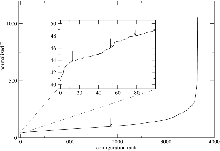
Figure 3: For the optimization of the most extended configuration of the IRAM interferometer, we show the $F$ parameter versus the final ranking of all the possibilities the code calculated. The highest ranking configurations are shown in the inset, where $F$ is lowest. The beams and $uv$ coverage of the 4 marked points are shown in Fig. 4.

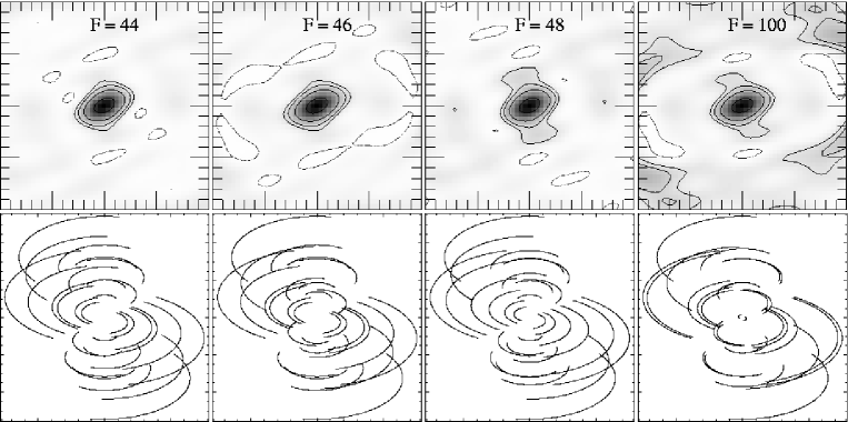
Figure 4: A demonstration of the convergence of our method, moving from right to left. The beams from 4 configurations sampled from Fig. 3, for a source at declination $+20\arcdeg$. The scale of the beam is that of Fig. 2. The $uv$ plane has a radius of 760 m.

Figure 2 shows the beam achieved by the new optimized A configuration of the IRAM interferometer. The beam shown results from a 9-hour observation of a $+45\arcdeg$ declination source per configuration. It demonstrates also that despite the optimization being carried out for $+20\arcdeg$ declination sources, the quality remains good at higher declinations. The two panels of the figure are shown at a scale of the primary and synthesized beams (left/right). Our method not only results in a beam with good imaging properties in an absolute sense, but also results in a rounder beam with lower sidelobes compared to the previous most extended configuration in this array.

For the specific optimization described here, there is only a limited number of possible antenna moves, since three antennas were anchored to the most extended positions. For that reason it was feasible to write to disk all the values of $F$ during the search. We have ranked all the configurations that our method has considered in the above optimization process, according to the $F$ parameter, with the best configuration (minimum $F$) assigned rank 1. In Fig. 3 we plot $F$ versus the rank (here we have normalized $F$ by $N_{V}(N_{V}-1)$). Although the curve is quite flat up to rank $\approx 3600$, a visual inspection of the beams shows that the quality deteriorates gradually but noticeably. The inset of Fig. 3 shows the best configurations according to our criterion. The 4 marks on this figure denote the configurations which we use to demonstrate the convergence of our method. In Fig. 4 we show the beams and $uv$ coverage of these four configurations. The quality of the beam obviously improves in terms of sidelobe levels from right to left. Although it is hard to rank these examples in terms of their $uv$ coverage by a simple visual inspection, our method identifies the left-most case as most “uniform”. The left most example also produces the lowest sidelobe levels. This is a clear demonstration that the optimization in the $uv$ plane results in a good quality beam in the image plane.

3.2 Adapting the very extended array of the SMA

Figure 5: The location of the 24 pads of the SMA. The circles denote the chosen pads for a six element, very extended array. The square and triangle show the pads identified in this work, which optimize this array in the case of seven and eight elements respectively. The phase center is at pad 1.

The Submillimeter Array (SMA) is located near the summit of Mauna Kea, on the Island of Hawaii, at an altitude near 4080 m. The SMA is comprised of eight 6-m diameter submillimeter-capable radio telescopes. The initial Smithsonian concept for the SMA was for six telescopes, but in 1996 the Academia Sinica Institute of Astronomy and Astrophysics (ASIAA) joined the project by agreeing to add two more telescopes (Ho et al., 2004).

There are currently 24 pad locations for the SMA, with the first 21 determined when the array was scheduled to consist of six elements. The locations were based on the work of Keto (1997), including the use of the Reuleaux triangles for optimization. The scheme utilizes four nested ”rings” of pads (see Fig. 5), with each ring providing a different spatial coverage and resolution. The addition of the two ASIAA telescopes was accomodated within the Reuleaux triangle scheme on an ad hoc basis, resulting in an additional three pads for configurations within the three smallest nested rings (Ho, Moran, and Lo 2004).

The highest spatial resolution array (called the ’very extended array’ and denoted in Fig. 5 as SMA pads 1, 17, 18, 19, 20, and 21) did not have additional pads added, and relies on the use of preexisting pads. This situation provides an opportunity to apply the concepts developed in this work. The specific question to be addressed is: given the original six pad locations for the very extended array, which two additional pads optimize the $uv$ coverage while minimizing degradation to spatial resolution. A secondary, related question is which pads are best if there are less than the full complement of eight telescopes (for example, if one is undergoing renovation or servicing).

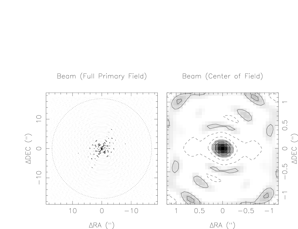
Figure 6: The synthesized beam of the six element, very extended SMA array, for a source at a declination of $+30\arcdeg$, shown at the level of the primary field and the size of the synthesized beam. Countour lines are at the same levels as in Fig. 2.

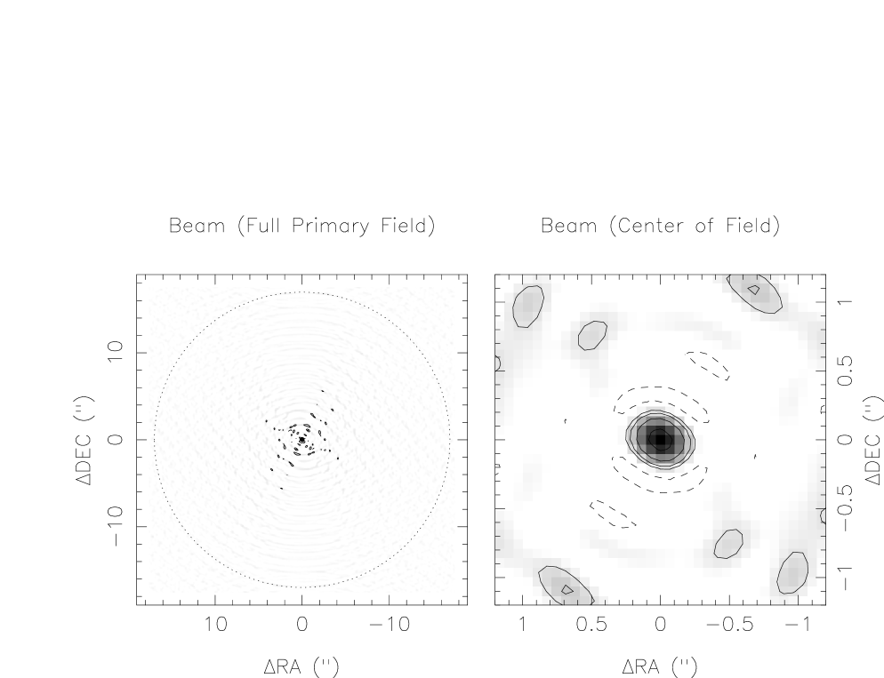
Figure 7: The synthesized beam of the very extended SMA array, with a total of 7 antennas. The beam retains its shape and the sidelobes are supressed compared to the six element array.

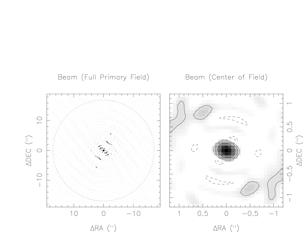
Figure 8: The synthesized beam of the very extended SMA array, with a total of 8 antennas. The sidelobes are further supressed compared to the six and seven element array.

The methods used in this work were applied to address these questions, and we find that if seven telescopes are available, the addition of pad 16 to the original very extended configuration provides the best $uv$ coverage, and if eight telescopes are available, the addition of pads 13 and 16 together is best. This optimization appears to hold true for a wide variety of source declinations, though does change slightly for very low (below $-25\arcdeg$) declinations. Figure 6 shows the synthesized beam obtained for the original six element configuration, for a declination of $+30\arcdeg$ at 345 GHz. Figures 7 and 8 show the improvement in the beam (primarily in suppression of sidelobes) for the seven element and eight element configurations, respectively. It is worth noting that the solution for the seven element case obtained rapidly here, was previously determined by SMA staff through a laborious search of possibilities using their synthesis beam generation tools. We consider the agreement in the two methods as confirmation that both correctly address the problem at hand, despite the fact that they are completely different in approach.

4 Conclusions

We have applied a simple principle, based on the ideas of Keto (1997) and Boone (2001, 2002), to develop a procedure that identifies configurations with good $uv$ coverage for low density interferometers with defined pads. The method has been put to the test in the particular situation where new antenna pads are available at the IRAM interferometer, which require a new set of antenna configurations. It has also been applied to identify configurations for the SMA with different numbers of antennas. Gaining or losing pads or antennas are events that are by no means unlikely for interferometric telescopes that apply multiple configurations.

The total number of configurations in which any interferometer observes is defined not only by scientific principles, but also by practical constraints. If the total number of possible configurations changes at some point in time, a new entire set of configurations will need to be redefined, and the method presented here is suitable to solve this problem in a fast and elegant way.

In summary, we propose here a fast method for optimizing the positions of antennas in an interferometric array with defined pads, as opposed to the method of Boone where antennas can be moved around on a real landscape. Our method resembles the method of Boone in that it consists of a repetition of a two step process: changes are made to antenna positions and the new configuration is evaluated. For the first part, our parameter space is finite so we explore it entirely, unlike the Boone method which explores part of the infinite space and converges to one of many possible solutions. Regarding the second step of the process, our method can be applied to interferometers with a low density of $uv$ samples, in contrast to the method of Boone, which only works for high density. Finally, a two-step procedure to define configurations in high density interferometers with defined pads can be developped, where the first step is taken from the method described here, and the second from the method of Boone. That would involve looping through all the possible configurations and ranking them by means of the Gaussian method described in Section 2.2.

References

- Boone (2001) Boone, F. 2001, A&A, 377, 368
- Boone (2002) Boone, F. 2002, A&A, 386, 1160
- Conway (2000a) Conway, J. 2000a, in ALMA memo, No. 283
- Conway (2000b) Conway, J. 2000b, in ALMA memo, No. 292
- Cornwell (1986) Cornwell, T. J. 1986, in ALMA memo, No. 38
- Cornwell (1988) Cornwell, T. J. 1988, IEEE Trans. Antennas Propagat., 36, 1165
- Cornwell et al. (1993) Cornwell, T. J., Holdaway, M. A., & Uson, J. M. 1993, A&A, 271, 697
- Guilloteau et al. (1992) Guilloteau, S., Delannoy, J., Downes, D., et al. 1992, A&A, 262, 624
- Ho et al. (2004) Ho, P. T. P., Moran, J. M., & Lo, K. W. 2004, ApJL, 616, L1-L6
- Keto (1997) Keto, E. 1997, ApJ, 475, 843
- Kogan (1997) Kogan, L. 1997, in ALMA memo, No. 171
- Thompson et al. (1991) Thompson, A. R., Moran, J. M., & Swenson, G. W. 1991, Interferometry and synthesis in radio astronomy (Malabar, Fla. : Krieger Pub., 1991.)
- Woody (1999) Woody, D. 1999, in ALMA memo, No. 270