The buildup of stellar mass and the 3.6 $\mu$m luminosity function in clusters from $z=1.25$ to $z=0.2$.

We have measured the 3.6 $\mu$m luminosity evolution of about 1000 galaxies in 32 clusters at $0.2<z<1.25$, without any a priori assumption about luminosity evolution, i.e. in a logically rigorous way. We find that the luminosity of our galaxies evolves as an old and passively evolving population formed at high redshift without any need for additional redshift-dependent evolution. Models with a prolonged stellar mass growth are rejected by the data with high confidence. The data also reject models in which the age of the stars is the same at all redshifts. Similarly, the characteristic stellar mass evolves, in the last two thirds of the universe age, as expected for a stellar population formed at high redshift. Together with the old age of stellar populations derived from fundamental plane studies, our data seems to suggest that early-type cluster galaxies have been completely assembled at high redshift, and not only that their stars are old. The quality of the data allows us to derive the LF and mass evolution homogeneously over the whole redshift range, using a single estimator. The Schechter function describes the galaxy luminosity function well. The characteristic luminosity at $z=0.5$ is is found to be 16.30 mag, with an uncertainty of 10 per cent.

1 Introduction

The luminosity function (LF) is the basic statistic used to understand galaxy properties, giving the relative frequency of galaxies of a given luminosity in a given volume. Most additional parameters determined for samples of galaxies having more than a single value of luminosity are usually averages weighted by the LF (in addition to underlying selection effects). Furthermore, by comparing the LF at different redshifts or environments it is possible to infer how galaxy luminosity evolves.

Since starlight at 3.6 $\mu$m very nearly follows the Rayleigh-Jeans limit of blackbody emission for $T>2000$ K, the colors of both early- and late-type stars are similar. There is virtually no dust extinction at this wavelength either, since any standard extinction law predicts only a few percent of the extinction of optical wavelengths. The 3.6 $\mu$m light therefore traces the stellar mass distribution free of dust obscuration effects (Pahre et al. 2004). Thus, a useful approach to understanding how galaxies form is to track their growing stellar mass, measured through the evolution of the 3.6 $\mu$m LF.

Several previous studies addressed the luminosity evolution of galaxies in clusters in near-infrared bands, notably de Propris et al. (1999). They found that the $K$-band LF of 38 clusters up to $z=0.92$ is consistent with the behavior of a simple, passive luminosity evolution model in which galaxies form all their stars at high redshift and thereafter passively evolve. However, and perhaps because a standard cosmology was not in place at the time of that work, the authors do not address which of the other possible evolutionary scenarios are rejected by the data and at what confidence. Kodama & Bower (2003), Kodama et al. (2004) found results compatible with little evolution in stellar mass, but with large uncertainties.

The de Propris et al. (1999) results were anticipated (and also later confirmed) by the analysis of sub-samples of cluster galaxies: early-type or red galaxies have properties (mainly colour and location in the fundamental plane) consistent with a passive evolution model. However, red or early-type galaxies are biased subsamples of the whole galaxy population and are affected by the progenitor bias (van Dokkum & Franx 2001). Furthermore, clusters of galaxies are also know to host star forming galaxies (e.g. Butcher & Oemler 1985). The fraction of blue galaxies growing with redshift (see e.g. Butcher & Oemler 1985; Rakos & Shombert 1995; but see Andreon, Lobo & Iovino 2004 for a different opinion) makes results based on the red/early-type population less representative of the whole population as redshift increases. LF studies do not suffer from the progenitor bias, and they directly approach the more fundamental problem of studying the evolution of the whole sample of galaxies. Therefore, LF studies are preferable to measure the ensemble mass evolution. Furthermore, stellar populations may be old, as pointed out by several colour or fundamental plane studies, but at the same time galaxies may not have been completely assembled: since $z=1$ and the present-day, galaxies might have grown in mass through mergers. This key issue can be tested by comparing the mass function of galaxies at different redshifts.

The paper is organized as follow: Sec 2 presents the data; Sec 3 describes the sample of studied clusters. Sec 4 summarizes the method used to derive the LF. The LF and the mass evolution determination are computed in Sec 5. Sec 6 and 7 discuss and summarize the results.

Throughout this paper we assume $\Omega_{M}=0.3$, $\Omega_{\Lambda}=0.7$ and $H_{0}=70$ km s^-1 Mpc^-1.

2 Data & data reduction

2.1 IR data

IR data were obtained with the IRAC (Fazio et al. 2004) on the Spitzer Space Telescope (Werner et al. 2004). A 9 deg² SWIRE (Lonsdale et al. 2003) field was imaged. The exposure time is 4 $\times$ 30s.

The standard pipeline pBCD (Post Basic Calibrated Data, ver. 10.5.0) products delivered by the Spitzer Science Center (SSC) were used in this paper. These data include flat-field corrections, dark subtraction, linearity and flux calibrations. Additional steps included pointing refinement, distortion correction and mosaicking. Cosmic rays were rejected during mosaicking by sigma-clipping. pBCD products do not merge together observation taken in different Astronomical Observations Requests (AORs). AORs are therefore mosaicked together using SWARP (Bertin, unpublished), making use of the weight maps. Sources are detected using SExtractor (Bertin & Arnout 1996), making use of weight maps.

Star/galaxy separation is performed by using the stellarity index provided by SExtractor, which, being the posterior probability based on a neural network, outperforms cuts (linear discriminators) in object parameter space (Andreon et al. 2000), as expected (e.g. Bishop 1995). We conservatively keep a high posterior threshold ($class_{star}=0.95$), rejecting “sure star” only ($class_{star}>0.95$) in order not to reject galaxies (by unduly putting them in the star class), leaving some residual stellar contamination in the sample. This contamination is later dealt with statistically.

We checked the star/galaxy classification using a 0.3 deg² region deeply observed at Cerro Tololo Inter–American Observatory (CTIO) by taking images under sub-arcsecond seeing conditions (see sect 2.2). We compared the classification derived from 3.6 micron images with those of one of our CTIO data observed with sub-arcsec resolution. Only less than about 2 per cent of the objects classified as stars (using $class_{star}>0.95$) using IRAC images are actually resolved at the CTIO resolution, and are therefore mis-classified. This 2 per cent of stars corresponds to 0.1 per cent of all the sources detected at 3.6 $\mu$m in the same field (and brighter than 18 mag), i.e. a negligible minority overall. Therefore, our posterior probability threshold ($class_{star}>0.95$) does not reject galaxies by unduly putting them in the star class at an appreciable level. The residual stellar contamination from our choice of the posterior threshold is subtracted statistically, as in the optical (e.g. Andreon & Cuillandre 2002) or the near–infrared (e.g. Andreon 2001).

Images are calibrated in the Vega system, using the IRAC zero points provided by the SSC (and, in particular by G. Wilson.

From the inspection of the galaxy count distribution, the completeness magnitude at $[3.6]$ is $\sim 18$ mag. Objects brighter than 12.5 mag are often saturated. Therefore, from now on, only the range $12.5<[3.6]<18$ mag is considered. In sec. 5.3 we check how results are affected by a potential incompleteness at the faint end.

The average density of sources in a circle of the point spread area is around 0.004. Therefore, it is very unlikely that crowding is an issue in average density regions, and also in 10 to 100 times overdense regions, such as cluster cores. Only one of our clusters required an accurate setting of the SExtractor deblending parameters to split the few blended sources.

2.2 Optical imaging data

In this paper we used CTIO wide-field imaging to control the quality of Spitzer star galaxy classification, as mentioned above. We adopt here part of the same imaging data used in Andreon et al. (2004a). In brief, optical $R$– and $z^{\prime}$–band ($\lambda_{c}\sim 9000$Å) images were obtained at the CTIO 4m Blanco telescope during August 2000 with the Mosaic II camera. Mosaic II is a 8k$\times$8k camera with a $36\times 36$ arcminute field of view. Typical exposure times were 1200 seconds in $R$ and $2\times 750$ seconds in $z^{\prime}$. Seeing in the final images was between 0.9 and 1.0 arcsecond Full–Width at Half–Maximum (FWHM). Data have been reduced in the standard way (see Andreon et al. 2004a for details). Typical completeness magnitudes are $R=24.5$, $z^{\prime}=23$ mag ($5\sigma$) in a 3 arcsec aperture.

3 The cluster sample

Figure 1: Richness for our clusters. The dotted line marks the typical $N_{0}$ of $R=0$ or $1$ cluster in the present day Universe, from Bahcall (1977).

The cluster sample studied in this paper consists of 32 colour–selected clusters, all spectroscopically confirmed. The clusters were detected as spatially localized galaxy overdensities of similar colour, as described in Andreon et al. (2003; 2004a,b). The detection method used takes advantage of the observation that most galaxies in clusters share similar colours, while background galaxies have a variety of colours, both because they are spread over a larger redshift range and because the field population is more variable in colour than the cluster one, even at a fixed redshift. All clusters but one were detected using $R-z^{\prime}$ colour; one cluster was detected using the $z^{\prime}-K$ colour because of its larger redshift (sec 3.2 of Andreon et al. 2005 for details about the latter cluster). After colour detection, the cluster nature of the studied clusters was confirmed with spectroscopic observations. The clusters are individually presented and studied in Valtchanov et al. (2004), Pierre et al. (2005), Willis et al. (2005), Andreon et al. (2004a, 2005a,b).

Altough studied clusters are colour–selected, 29 out 32 of the clusters are also x-ray detected, leaving only 3 clusters (at $z=0.49,0.61$ and at $z=1.02$) with too faint x-ray emission to be detected with 10 to 20 ks XMM images. The detected x-ray emission guarantees that the studied clusters have deep potential wells and independently confirms the cluster nature of the studied objects.

The studied cluster sample is not a volume complete sample, nevertheless it densely samples the explored Universe volume, up to $z\sim 1$. Assuming the local (Ebeling et al. 1997) $L_{X}$ luminosity function, we found that the expected number of clusters with x-ray luminosity $L_{X}>10^{43}$ erg/s up to $z\approx 1$ and with more than 50 counts on 10 ks XMM images is about 15 per deg². All 32 studied clusters are in a contiguous 2.8 deg² area of the sky, and therefore the cluster number density is about 11 clusters per deg². The high number density of clusters should make the studied sample somewhat representative of typical clusters, making any bias of the studied sample small.

In order to characterize the cluster richness, for each cluster we compute the number of galaxies inside a radius of 357 kpc (corresponding to 500 kpc in the old cosmology and in the nearby universe studied by Bahcall 1977) brighter than $m^{*}+1.7$ (corresponding to Bahcall $\sim m_{3}+2$ for an $\alpha=-1$ Schechter function). The background contribution has been removed (marginalized) using Bayesian techniques described in Appendix B of Andreon et al. (2005). Here we quote the mean of the posterior and its rms as a measure of the cluster richness and its error, respectively, for a uniform prior (but results are similar using a Jeffreys prior). Clusters of Abell (1958) richness 0 or 1 in the present–day Universe have $N_{0}$ of about 15 to 20 (Bahcall 1977). Figure 1 shows that two thirds of our clusters have $N_{0}<20$ galaxies. Most of the clusters with $N_{0}>20$ galaxies have large error bars, which make them consistent with $N_{0}=20$ galaxies at two sigma. Therefore, most of our clusters are at the bottom of the Abell richness scale and are not rich systems.

The 32 clusters are distributed in the redshift ranges in the following way (see also Figure 2): 13, 8, 5, 6 clusters are in the range: $0.25<z<0.40$, $0.40<z<0.65$, $0.75<z<0.90$ and $0.99<z<1.25$, respectively.

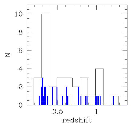
Figure 2: Redshift distribution of the studied clusters. Solid/open histograms mark 0.01/0.1 bin width in redshift.

4 The method: LF determination

We do not attempt here, as in some previous approaches, to infer the luminosity function from an optically selected sample, because the latter option assumes the absence of very dust obscured objects: if galaxies are dust obscured enough to go undetected in the optical, their contribution to the IR LF is deemed to be zero, when instead it may be relevant. Some previous authors were forced to assume the absence of very dust obscured objects, because they need spectroscopic redshifts, mostly acquired in the optical window, or because they need multi–colour optical photometry to determine a photometric redshift. Here, instead, we use the approach usually adopted for clusters, where knowledge of the individual galaxy redshift is not used.

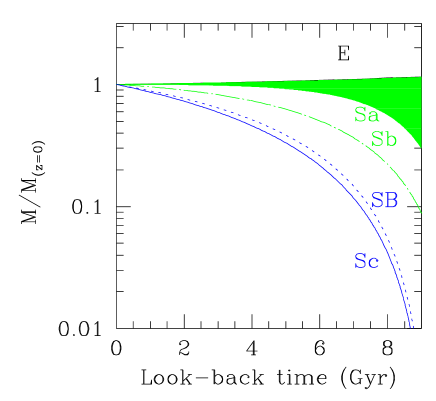
Figure 3: Stellar mass evolution for several stellar mass growth models (curves) and as derived from our data (shaded area). The region allowed by the data is part of the shaded green area derived in sec 5.2.

In order to compute the LF we adopt two different methods.

– For display purposes only, the LF is computed as the difference between the (binned) counts in the cluster and control field direction, as usual (e.g. Zwicky 1957, Oemler 1973). Error bars are computed as the square root of the variance of the minuend, because the contribution due to the uncertainty on the true value of background counts is negligible. A negative number of cluster galaxies may occur in the presence of a low cluster signal and Poissonian fluctuations, which leads to the unphysical result of negative numbers of cluster galaxies when data are binned.

– Second, we fit the unbinned galaxy counts, without any use of binned data or errors computed in the previous approach. We are faced with the classical statistical problem of determining two extended (integral$>1$) density probability function, one carrying the signal (the LF of cluster members) and the other being due to a background (background galaxy counts, BKG) from the observations of many individual events (the galaxies luminosities), without knowledge of which event is the signal (which galaxy is a member) and which one is background. Here, we follow the rigourous method set forth in Andreon, Punzi & Grado (2004, APG hereafter), which is an extension of the Sandage, Tammann & Yahil method (1979, STY) to the case where a background is present, and that adopts the extended likelihood instead of the conditional likelihood used by STY. The method does not remove the background from the data, but adds a component (the background) to the model. The method also provide the normalization (at the difference of STY), needed to rigorously combine the LF of the individual clusters, properly accounting for the uncertainty in the LF normalizations. 68 per cent confidence intervals are derived using the Likelihood Ratio theorem (Wilks 1938, 1963) made known to the astronomical community by Avni (1976) and Press et al. (1986), among others. The method comes in two forms: in sec 5.1 we neglect astronomical and statistical subtleties, proceeding in the analysis as most previous published papers, whereas in sec 5.2 we take a fully rigorous approach, and we describe its advantages with respect to the simpler application.

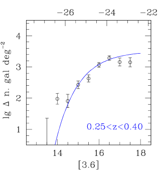
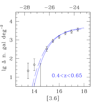
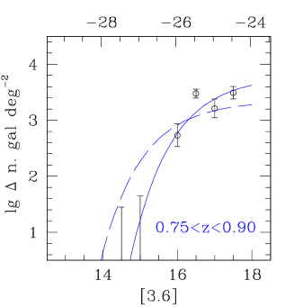
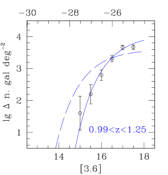
Figure 4: Composite LF in the $[3.6]$ band as a function of apparent (lower abscissa) and absolute (upper abscissa) magnitudes. Data points and error bars are computed as usual (e.g. Oemler 1973, see sec 4). The solid and long dashed curves are fit to unbinned counts, but neglecting astronomical and statistical subtleties, as described in sec 5.1. The solid curve refers to a fit with $m^{*}$ free, whereas the dotted curve is a fit with $m^{*}$ held fixed to the value observed at $0.25<z<0.40$. All these LF determinations are superseded by the LF determined in sec 5.2, which is a rigorous fit over all cluster and field data.

4.1 Background and cluster areas

As the background field we considered a central 4 deg² region for simplicity, and we fit the background counts with an arbitrary function. In this region, there are about 106000 objects. The average background is therefore very well determined, because it is measured over a large area with respect to the cluster area. Its determination is so good that galaxy counts in the cluster direction (an area about 750 times smaller) does not constrain the background counts at all. Therefore, it is justified here to keep the background parameters at the best fitting values observed in the control field (but see APG for why this is unjustified in general).

For all but 2 clusters, we measured the LF within a circle of 5 arcmin aperture. For the remaining two clusters an aperture of 3 arcmin is taken because of incomplete data coverage or because of a bright nearby star. This aperture is similar to the one used in the optical LF determination for several clusters in common with Andreon et al. (2004a), and it has been chosen as a compromise between sampling the whole cluster and not including a too large contribution from background galaxies.

4.2 Evolutionary models

In order to estimate the expected apparent magnitude, absolute magnitude and mass to light ratio for different galaxy models having various growth histories we used GRASIL (Silva et al. 1998; Panuzzo et al. 2005), which is a code to compute the spectral evolution of stellar systems taking into account the effects of dust, which absorbs and scatters optical and UV photons and emits in the IR-submm region. We adopt standard elliptical (E), Sa, Sb, Sc and Arp 220 (SB) models with default parameters (Silva et al. 1998): a Salpeter initial mass function is used, with lower/upper limit fixed to 0.15/120 $M_{\odot}$. We assume that no stars are formed from $z=\infty$ to $z=5,2,2,1.5,1.5$ for E, Sa, Sb, Sc and SB models, respectively. The models fully account for evolving metallicity and dust content with dust mixed to stars (see Silva et al. 1998 for details). Figure 3 shows model mass growth histories appropriate for an object having currently broad band spectrophotometry typical of E, Sa, Sb, Sc and star burst (SB) galaxies. The E model of stellar mass growth history is characterized by the absence of recent stellar mass growth, while later types display recent episodes of stellar mass growth. These stellar mass growth histories are not intended to represent the stellar mass growth history of an individual object, but only of the average class, which is why these curves are smooth, while the mass growth of individual object is more erratic.

5 Results

5.1 A simplistic approach

We start with a simple analysis of the data, without statistical and astronomical subtleties. We largely follow the usual astronomical method of LF computation in the field and also in the cluster when many clusters are available. First, we bin data in redshift bins. In this step we ignore that the redshift bin is of non–vanishing width (i.e. we overlook the required convolution of the model by the appropriate redshift kernel) and that sources likely brighten in their rest–frame due to the younger age of stars going from the near to the far side of the redshift bin. We also overlook some statistical subtleties (each cluster has a Schechter function, not just the composite), and logical coherence (we are attempting to measure the evolution assuming its absence, as most previous works did, and as criticized by Andreon 2004). A fully rigorous analysis is presented in section 5.2.

There are 260, 250, 100 and 240 cluster (i.e. background subtracted) members inside the composite clusters at $0.25<z<0.40$, $0.40<z<0.65$, $0.75<z<0.90$ and $0.99<z<1.25$, respectively.

As a model for the cluster LF we adopt a Schechter (1976) function:

$$\phi_{i}(m)=\phi^{*}_{i}10^{0.4(\alpha+1)(m^{*}-m)}e^{-10^{0.4(m^{*}-m)}}$$ (1)

where $m^{*}$, $\alpha$ and $\phi^{*}_{i}$ are the characteristic magnitude, slope and normalization, respectively. The index $i$ refers to the cluster $i^{th}$. In this section, we fixed the Schechter slope $\alpha$ to $-1$ because it is largely undetermined.

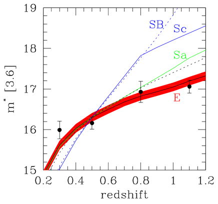
Figure 5: The different lines shows the apparent magnitude of a galaxy having $[3.6]=16.3$ mag at $z=0.5$, depending on stellar mass growth histories, as labelled, as well as for an unphysical model where galaxies have the same old age at all redshifts (dotted black line). Data points are $m^{*}$ values derived in sec 5.1. The red region marks the observed 68 per cent confidence bound of $m^{*}$ derived in sec 5.2.

Figure 4 shows the LF in each redshift bin. Data points and error bars are computed as usual (e.g. Oemler 1973). When the difference between the cluster and control field counts is negative the result cannot be plotted, because the logarithm function requires a positive argument. The solid curve is the LF of the composite dataset, obtained by fitting the unbinned counts in the composite cluster and control field directions. We do not fit the displayed data points shown in the figure, and the LF fit (parameter or error determination) makes no use of these data points and errors, and they are shown for display purposes only: we fit, as mentioned, unbinned counts in the cluster and control field directions.

The ‘data’ points nicely follow the Schecther function. As redshift increases, the LF moves to the right, i.e. $m^{*}$ becomes fainter in the observer frame, by about 1.0 mag between $0.25<z<0.40$ and $0.99<z<1.25$. In all redshift panels also plotted, as a long-dashed curve, is a fit with $m^{*}$ held fixed to the value observed in the lowest redshift bin. High-redshift data reject a model with $m^{*}$ held fixed to the value observed in the lowest redshift bin.

Figure 5 shows the expected apparent magnitude of a galaxy having $[3.6]=16.3$ mag at $z=0.5$, for some stellar mass growth histories. It shows that a minimum of 1.5 mag of fading is expected in apparent magnitudes going from $z=0.3$ to $z=1.1$, whereas only 1.0 mag of fading is observed. However, it is not obvious from this figure whether the data reject the various stellar mass growth histories and at what confidence. We will not pursue the statistical computation using the approximate method just described, but using the rigorous method detailed in the next section.

5.2 Adding rigour

Deriving luminosity evolution after having assumed that it is equal to zero in each studied redshift bin (i.e. the approach of the previous section) makes use of a circular argument: the computation of the LF assumes a model for galaxy evolution, that unfortunately is precisely what the LF is used to measure. This occurs even for the traditional manner in which the LF is computed: having observations at different redshifts (look-back times) and desiring to measure how galaxies evolve, we should count galaxies having a given absolute mag at, say, $z=1$ with galaxies having the same absolute mag at, say, $z=0$ (and in such a case we assume that galaxy luminosity does not change with look-back time), or with galaxies having a different luminosity (and in such a case we assume a given evolution). And, if we know how the luminosity evolves (because this is needed to make the computation), there is no need to perform the experiment (why measure the LF?).

Beside the logical inconsistency, the assumption of a level of evolution underestimates error bars by a significant factor, as measured in an actual case by Andreon (2004). We stress that a rigorous method is required if one wants to be sure of the correctness of the result, and, when the number of members in a given mag bin, estimated from the difference of galaxy counts in the cluster and control field directions, leads to unphysical (negative) values. One should, instead, solve for background counts, for the LF and its evolution at the same time, without binning the sample in redshift bins and without bin the data in magnitude bins. This can be achieved adopting a more complex model in which additional parameters account for the evolution, following the path in previous works (Lin et al. 1999, Blanton et al. 2003, Andreon 2004) and reinforced in APG.

Algeabrically, $m^{*}$ in Eqn. 1 is replaced by:

$$m^{*}_{z}=m^{*}_{z=0.5}+\Delta m_{model}-Q\ (z-0.5)$$ (2)

where $\Delta m_{model}=m_{model}-m_{model,z=0.5}$.

Thus, we make the $m^{*}$ model fainter by an amount given by the prediction appropriate for the adopted stellar mass growth history and cosmology and we allow a supplementary linear evolution (i.e. proportional to redshift), normalizing everything to $z=0.5$ to make corrections equal to zero at roughly the median redshift of our survey.

Our $Q$ has a different meaning from $Q$ in Lin et al. (1999), Blanton et al. (2003) and Andreon (2004): here $Q=0$ means that galaxies form stars according to the model, whereas in the former works $Q=0$ means that the luminosity stays constant over time, which is, of course, unphysical.

The sample consists of about 5500 galaxies, of which about 950 galaxies are in clusters, and the remaining are interlopers.

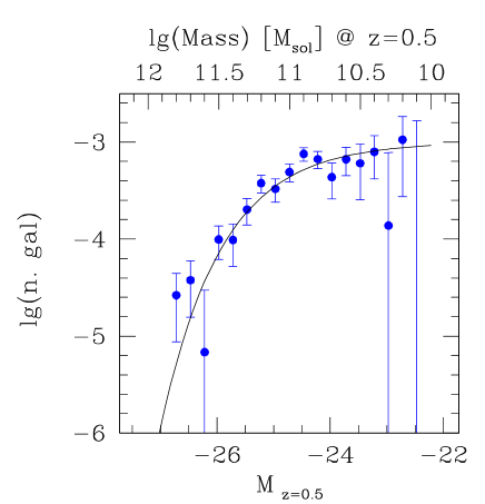
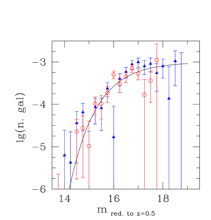
Figure 6: Best fit LF at $z=0.5$. Left: LF of the whole sample. Right: LF of the lower and upper redshift halves (blue closed triangles and red open circles, respectively). The match of the two halves occurs only if the assumed evolution is the correct one.

To compute the LF, we start with model selection. We use two statistical tests: the likelihood ratio test (LRT) will inform us of how frequently one incorrectly rejects the null hypothesis, under the hypothesis that the null is true. The Bayesian Information Criteria (BIC, Swartz 1978; Lindle 2004 provides a useful astronomical introduction) informs us about the relative evidence of two models. LRT cannot be used when regularity conditions required for its application do not hold (for example, compared models should be hierarchically nested, i.e. one model should be a particular case of a more general model).

We compare the E model to the other models, all with fixed $Q=0$, irrespective of the $m^{*}$ and $\alpha$ values. BIC provides very strong support for the E stellar mass growth history ($\Delta BIC\ga 5$ for Sa, and larger values for the other models). Our statistical analysis offers the advantage of avoiding an unnecessary assumption about the value of the best fit parameters in order to identify the most likely evolutionary model: it is able to infer an evolutionary model without any assumption about the $\alpha$ value, while such an assumption was done in sec 5.1 and in previous works, because these studies were forced to fix the $\alpha$ parameter to derive the evolution of $m^{*}$. Not fixing the $\alpha$ value, our approach is not affected by the known correlation between $m^{*}$ and $\alpha$ that plagued previous approaches.

Figure 3 summarizes the above model comparison: the acceptable area (i.e. the constraint put on models by our data) is a part of the shaded (green) area plotted in Figure 3, ie. the region between the E track (a good description) and the Sa track (a bad one). The major difference between the Sa track (rejected by the data) and E track begins at look–back times greater than 7 Gyr, i.e. at $z>0.85$, and becomes large at look–back times greater than 7.5 Gyr (i.e. $z\ga 1$). We can discriminate between the two models because we have 8 clusters at $z>0.85$ and 5 clusters at $z>0.99$, where models differ the most (Fig 3).

We now verify whether the model is a) too complex (too many unconstrain parameters) for the data in hand, and b) if the data requires that the E model should be updated with a better one. We compare the E model having fixed $Q=0$ and $\alpha=-1$ to more general E models with $Q$ or $\alpha$ free. BIC and LRT both inform us that the simplest model is favored. Given the data in hand, the E model does not need to be refined by the addition of a linear (with redshift, i.e. a $Q$) term. Furthermore, the $\alpha$ parameter is largely unconstrained, quantifying what is qualitatively apparent in Fig. 4.

BIC strongly rejects the unphysical universe (the track of an E with the present-day age at all redshifts).

The final best fit model is therefore the one of an old and passively evolving population formed at high redshift, without any additional recent stellar mass growth (i.e. the E model and $Q=0$). For $\alpha=-1$ (the best formal fit is $\alpha=-1.05$, but with large error bars), we found $m^{*}_{z=0.5}=16.30\pm 0.10$ mag, i.e. $M^{*}=-24.8,-24.9,-25.1,-25.3$ mag at $z=0.3,0.5,0.8,1.1$.

Figure 6 shows the rigorously derived best fit LF (the curve) at $z=0.5$ and the data points. Having measured the luminosity evolution, we can now safely assume it in order to combine counts at different redshifts (look–back times). We normalize each individual LF by the model $\phi^{*}_{i}$ value, and we then weight each cluster by its $\phi^{*}_{i}$ value, after having evolved magnitudes from the cluster redshift to our reference redshift, $z=0.5$. In doing this convolution we keep only bins entirely included in the studied magnitude range, for simplicity. As in literature approaches, errors on the data points do not include data combining errors (whereas they are accounted for in our rigorous derivation, see APG). There is a good agreement between the curve and the data points, meaning that the Schechter function is a good description of the LF over the observed magnitude range, and that the selected stellar mass growth history provides a good description of the observed evolution. The latter point is displayed in the right panel of Figure 6. It shows the LF by splitting the sample in two redshift halves, at median redshift. The two LFs share a common $m^{*}_{z=0.5}$, and this occurs only if we selected the right stellar mass growth history model: if the adopted model underestimates the luminosity evolution in one of the halves, two different (horizontally shifted) LFs would be observed (as we discuss later). This “result” is a visual check of the model selection already discussed.

Figure 7 qualitatively shows why we have ruled out the evolution of a stellar population whose stellar mass growth history is appropriate for an Sa (or later types): it displays the LF of clusters at $z<0.85$ and $z>0.85$, separately, evolved to $z=0.5$ assuming the stellar mass growth history of an Sa population. The $m^{*}_{z=0.5}$ of the two samples do not match, as emphasized by the bottom panel that shows the cumulative LF: the high-redshift LF is left-shifted (too bright) with respect to the low-redshift LF, contrary to the adopted hypothesis that evolution is well described by the adopted stellar mass growth history. The mass evolution allowed by the data is much quieter than that of an Sa galaxy. The model selection performed confirms this result rigorously, quantifying its statistical significance.

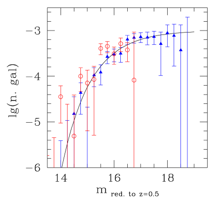
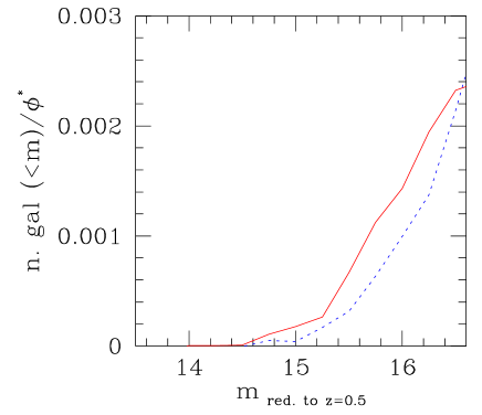
Figure 7: Top panel: LFs, evolved to $z=0.5$ assuming an Sa stellar mass growth history, of the lower and upper redshifts ranges (marked by blue closed triangles and red open circles for $z<0.85$ and $z>0.85$, respectively). The mismatch between the two LFs (circles are left-shifted) implies that the assumed stellar mass growth history is rejected by the data. Bottom panel: blow-up of the cumulated LF, better showing the LF mismatch.

Having identified the evolutionary model, we can convert absolute magnitudes into a stellar mass scale, using the $\mathcal{M}/L$ ratio of the model. The mass scale is shown as the upper abscissa in Fig 6. We found $\mathcal{M^{*}}=1.1,1.2,1.2,1.2\ 10^{11}M_{\odot}$ at $z=0.3,0.5,0.8,1.1$, respectively, were $\mathcal{M^{*}}=M^{*}(\mathcal{M}/L)_{model}$ (in the appropriate units). The statistical accuracy is 10 per cent, derived from the $m^{*}$ uncertainty only. The absolute value of the characteristic mass, $\mathcal{M^{*}}$, depends on several key model parameters (e.g. the lower mass limit of the initial mass function, see Bell & de Jong 2001), while its evolution does not, as long as model parameters are redshift-independent.

Thus, we found that the luminosity of our galaxies evolves as an old and passively evolving population formed at high redshift. Models with a prolonged stellar mass growth are rejected by the data with high confidence. The mass function does not change in the last 8 Gyr, corresponing to the two thirds of the current Universe age. The data also reject the need for a redshift-dependent description of the evolution more accurate than a passively evolving population formed at high redshift (i.e. a $Q\neq 0$ is rejected). The data also reject models in which the age of the stars is the same at all redshifts. The Schechter function well describes the data.

It makes little sense to improve upon these constraints with our data alone, say to attempt to constrain the characteristic time scale of the mass growth because of a degeneracy: the same luminosity evolution may be produced by an older, but longer, episode of star formation, or a younger but shorter one.

5.3 Test on incompleteness

In order to test the effect of a potential incompleteness of the sample at [3.6] $\sim 18$ mag, we cut the sample at $12.5<[3.6]<17.5$ mag, and we compute $m^{*}$ for the E model and $Q=0$. We found $m^{*}=16.54\pm 0.11$ mag, in good agreement with the value measured by considering the larger sample [3.6]$<18$ mag, $16.30\pm 0.10$ mag. Application of BIC still favour the E model over Sa and later type ones, but now at lower significance ($\Delta BIC\ga 3$) because of the reduced sample size. Tus, the potential incompleteness of the sample at [3.6] $\sim 18$ mag is too small to affect the results of our analysis.

6 Discussion

6.1 Comparison with previous works

There are no LFs in the [3.6] band with which we can directly compare, and therefore, we compare our [3.6] LF with LFs derived at shorter wavelengths. Our measure of evolution at 3.6 $\mu$m is a luminosity–weighted measure of evolution. The advantage of the chosen band is that it is far less sensitive to sporadic star formation episodes involving a small fraction of the mass than similar determinations performed at shorter wavelengths, because the [3.6] band measures the flux emitted between the $H$ (at $z=1.25$) and $K$ (at $z\sim 0.1$) band rest-frame. At these wavelengths the flux-weighted age of a simple stellar population from Bruzual and Charlot (2003) is about 5 Gyr (e.g. Martin et al. 2005). Instead, in the B band rest-frame, the flux-weighted age is 1.5 Gyr, and drops by a factor of 10 at $\lambda\sim 3000$ Å . Therefore, comparison of results obtained in different bands requires that we pay attention to the considered wavelengths.

Luminosity evolution derived in the [3.6] and $K$ bands can be directly compared, because both determinations are sensitive to the same long-lived stars. Toft et al. (2004) summarized the cumulative efforts in the literature (largely relying on de Propris et al. 1999) to determine the LF at $z\ga 0.1$. Our data alone match in number and in redshift distribution this cumulate effort. Toft et al. (2004) and de Propris et al. (1999) both find that the redshift dependence of $m^{*}$ agrees with that of a passively evolving population formed at high redshift, as we have found and as also found by Kodama & Bower (2003) and Kodama et al. (2004). To quantitatively compare values derived in different bands, we need to determine $m^{*}_{z=0.5}$ for the same slope adopted in the comparison work ($\alpha=-0.9$, because most of the measurements have been performed with such a slope), and to convert our $m^{*}_{z=0.5}$ from [3.6] to the $K$ band. To perform the latter task we use model $K-[3.6]$ colors provided by Grasil. The best fit value converted to the $K$ band is $m^{*}_{z=0.5}=16.7\pm 0.1$, in good agreement with the value inferred from Fig. 11 in Toft et al. (2004) $m^{*}_{z=0.5}=16.6\pm 0.5$ mag. Our measure has a five times better accuracy than the latter, because Toft et al. (2004) do not fit $m^{*}$ to their data, but simply force $m^{*}$ to be equal to the value observed by de Propris et al. (1998) at $z=0$, thus inheriting its accuracy ($\pm 0.5$ mag). As mentioned in the introduction, our analysis rules out several alternatives (a non-passive evolution, for example), whereas Propris et al. (1999) do not address the topic of model selection, perhaps because of the freedom in cosmological parameters at the time of their analysis.

The LF study by Andreon et al. (2004) samples $\approx U$ and $B$ bands and their sample of clusters has a large overlap (13 clusters) with the one studied in this paper. They found that clusters are composed of two populations, one that had evolved passively from $z_{f}>2$, and one formed at lower redshift ($z_{f}<1$). The bands used trace, as mentioned, almost instantaneous star formation more than the stellar mass growth studied in this paper. The lack of a detection of a secondary stellar mass growth episode at [3.6] micron combined with its detection at shorter wavelengths implies that the mass involved in such episodes is small. Quantification of the mass involved will be reported elsewhere.

For the measurement of the stellar mass evolution, most of the literature works compare mass estimates derived from different estimators at different redshifts, because of the lack of similar measures (in the galaxy rest-frame) over a large redshift range. Instead, our measures are homogeneous and derived from a single estimator over the whole redshift range. Our mass evolution estimate may rely on the appropriateness of the adopted model (i.e. stellar mass growth history). However, we allow deviations from the model (several stellar mass growth histories and non-null $Q$ values), but the data rejected them. Furthermore, literature approaches also rely on stellar mass growth models, and to a larger degree than us, because they assume that the stellar mass growth history of each individual galaxy is well described by a simple model, whereas we assume that the above holds true for the average galaxy. Averages, by definition, are smoother and better described by a smooth model than individual measures.

Our results on evolution of the stellar mass in cluster galaxies are in broad agreement with the literature. Bundy, Ellis and Conselice (2005) find little evolution in the field from $z\sim 1$ to $z\sim 0$, with particular emphasis on bright (massive) objects better sampled in their (and in our) work. Our result also agrees with Kodama & Bower (2003) and Kodama et al. (2004), who claim that there has been little evolution in $\mathcal{M^{*}}$, but with large uncertainties, by comparing its value measured in cluster candidates and the $z\sim 0$ value (from Balogh et al. 2001), using heterogeneous mass estimators and data. Our sample of clusters at high redshift is larger than theirs (we have 6 spectroscopically confirmed clusters at $z>0.99$, vs 3 candidate clusters in Kodama & Bower 2003 and 5 candidate clusters in Kodama et al. 2004), and our comparisons use the same mass estimator and uniform data. Furthermore, spectroscopic observations presented in a very recent paper (Yamada et al. 2005) suggest that at least two of the Kodama et al. (2003) clusters are instead line of sight superpositions. The cluster nature of all our clusters has been spectroscopically confirmed, and, for all but three clusters, also confirmed through the detection of the cluster x-ray emission.

6.2 Early assembly and formation time of cluster galaxies

The evolution of the mass function of cluster galaxies only measures the evolution of the galaxy population as a whole and does not necessarily imply a direct correspondence to the evolution of individual galaxies. For example, the constancy of the mass function can be interpreted equally well as a combination of different and more complicated evolution of individual galaxies, some of which grow stellar mass (say, by mergers), and some that lose stellar mass. However, such a possibility is unlikely, because it requires two physical mechanisms with similar mass and time (i.e. redshift) dependencies, otherwise the stellar mass function would change. The simplest interpretation, supported by the existence of very massive ($\mathcal{M}>10^{11.5}M_{\odot}$) galaxies in our clusters, is that the mass assembly of most of galaxies in clusters (sampled with the available data) was largely complete at $z>1.25$.

Fundamental plane and colour studies (e.g. Bower et al. 1992; Stanford et al. 1998; Kodama et al. 1998; Andreon 2003; Andreon et al. 2004a; van Dokkum & Stanford 2003 and references therein) suggest that there is little recent star formation in early-type or red galaxies but does not tell us whether these galaxies have been completely assembled. As long as early-type or red galaxies are not a minority population in our clusters, the observed constancy of the mass function from $z=1.25$ to the present-day, as well as the old age of the stellar populations, implies that these galaxies have been completely assembled, and not only that their stars are old.

7 Summary

We had measured the 3.6 $\mu$m luminosity evolution of about 1000 galaxies in 32 clusters at $0.2<z<1.25$, without any a priori assumption about luminosity evolution, i.e. in a logically rigorous way. Our data match in number and in redshift distribution the cumulated literature effort thus far. The quality of the data allows us to derive the LF and mass evolution homogeneously over the whole redshift range, using a single estimator, at variance with previous determinations. We found that the luminosity of our galaxies evolves as an old and passively evolving population formed at high redshift without any need for a further redshift-dependent evolution. Models with a prolonged stellar mass growth are rejected by the data with high confidence. Data also reject models in which the age of the stars is the same at all redshifts. Similarly, the characteristic mass function evolves as a passively evolving stellar population formed at high redshift. The Schechter function describes the galaxy luminosity function well. The characteristic luminosity at $z=0.5$ is 16.30 mag with a 10 per cent uncertainty.

- (1)
- Abell (1958) Abell, G. O. 1958, ApJS, 3, 211
- Andreon (2001) Andreon, S. 2001, ApJ, 547, 623
- Andreon (2003) Andreon, S. 2003, A&A, 409, 37
- Andreon (2004) Andreon, S. 2004, A&A, 416, 865
- Andreon (2005) Andreon, S. 2005, in ”The fabulous destiny of galaxies: Bridging past and present”, (astro-ph/0509627)
- Andreon & Cuillandre (2002) Andreon, S., & Cuillandre, J.-C. 2002, ApJ, 569, 144
- Andreon et al. (2004) Andreon, S., Lobo, C., & Iovino, A. 2004, MNRAS, 349, 889
- Andreon et al. (2004a) Andreon, S., Willis, J., Quintana, H., Valtchanov, I., Pierre, M., & Pacaud, F. 2004a, MNRAS, 353, 353
- Andreon et al. (2004b) Andreon, S., Willis, J., Quintana, H., Valtchanov, I., Pierre, M., & Pacaud, F. 2004b, in the proceeding of ‘Rencontres de Moriond: Exploring the Universe. Contents and Structure of the Universe’ (astro-ph/0405574)
- Andreon et al. (2005) Andreon, S. et al. 2005a, MNRAS, 359, 1250
- Andreon et al. (2005) Andreon, S. et al. 2005b, MNRAS, submitted
- (13) Andreon, S., Punzi, G., Grado, A., 2005, MNRAS, 360, 727
- Avni (1976) Avni Y., 1976, ApJ 210, 642
- Bahcall (1977) Bahcall, N. A. 1977, ApJ, 217, L77
- Balogh et al. (2001) Balogh, M. L., Pearce, F. R., Bower, R. G., & Kay, S. T. 2001, MNRAS, 326, 1228
- Bell & de Jong (2001) Bell, E. F., & de Jong, R. S. 2001, ApJ, 550, 212
- Bertin & Arnouts (1996) Bertin, E., & Arnouts, S. 1996, A&AS, 117, 393
- Bishop (1995) Bishop C.M., 1995, Neural Networks for Pattern Recognition, Oxford UK: Oxford University Press
- Blanton et al. (2003) Blanton, M. R. et al. 2003, ApJ, 592, 819
- Bower et al. (1992) Bower, R. G., Lucey, J. R., & Ellis, R. S. 1992, MNRAS, 254, 601
- Bruzual & Charlot (2003) Bruzual, G., & Charlot, S. 2003, MNRAS, 344, 1000
- Bundy et al. (2004) Bundy, K., Fukugita, M., Ellis, R. S., Kodama, T., & Conselice, C. J. 2004, ApJ, 601, L123
- Butcher & Oemler (1984) Butcher, H., & Oemler, A. 1984, ApJ, 285, 426
- de Propris et al. (1998) de Propris, R., Eisenhardt, P. R., Stanford, S. A., & Dickinson, M. 1998, ApJ, 503, L45
- de Propris et al. (1999) de Propris, R., Stanford, S. A., Eisenhardt, P. R., Dickinson, M., & Elston, R. 1999, AJ, 118, 719
- Drory et al. (2004) Drory, N., Bender, R., Feulner, G., Hopp, U., Maraston, C., Snigula, J., & Hill, G. J. 2004, ApJ, 608, 742
- Ebeling et al. (1997) Ebeling, H., Edge, A. C., Fabian, A. C., Allen, S. W., Crawford, C. S., & Boehringer, H. 1997, ApJ, 479, L101
- Eisenhardt et al. (2004) Eisenhardt, P. R., et al. 2004, ApJS, 154, 48
- Fazio et al. (2004) Fazio, G. G., et al. 2004, ApJS, 154, 10
- Fontana et al. (2004) Fontana, A., et al. 2004, A&A, 424, 23
- Jeffreys (1938) Jeffreys, H. 1938, MNRAS, 98, 190
- Kodama et al. (1998) Kodama, T., Arimoto, N., Barger, A. J., & Arag’on-Salamanca, A. 1998, A&A, 334, 99
- Kodama & Bower (2003) Kodama, T., & Bower, R. 2003, MNRAS, 346, 1
- Kodama et al. (2004) Kodama, T., et al. 2004, MNRAS, 350, 1005
- Liddle (2004) Liddle, A. R. 2004, MNRAS, 351, L49
- Lin et al. (1999) Lin, H., Yee, H. K. C., Carlberg, R. G., Morris, S. L., Sawicki, M., Patton, D. R., Wirth, G., & Shepherd, C. W. 1999, ApJ, 518, 533
- Lonsdale et al. (2003) Lonsdale, C. J., et al. 2003, PASP, 115, 897
- Lonsdale et al. (2004) Lonsdale, C., et al. 2004, ApJS, 154, 54
- Martin et al. (2005) Martin, D. C., et al. 2005, ApJ, 619, L1
- Oemler (1974) Oemler, A. , Jr. 1974, ApJ, 194, 1
- Pahre et al. (2004) Pahre, M. A., Ashby, M. L. N., Fazio, G. G., & Willner, S. P. 2004, ApJS, 154, 235
- Panuzzo et al. (2005) Panuzzo, P., Silva, L., Granato, G. L., Bressan, A., & Vega, O. 2005, in ”The Spectral Energy Distribution of Gas-Rich Galaxies: Confronting Models with Data”, eds. C.C. Popescu and R.J. Tuffs, AIP Conf. Ser., in press, (astro-ph/0501464)
- Pierre et al. (2004) Pierre, M., Valtchanov, I., Altieri, B., et al., 2004, JCAP, 09, 011
- Press, Flannery, & Teukolsky (1986) Press, W. H., Flannery, B. P., & Teukolsky, S. A. 1986, Numerical Recipes, Cambridge: University Press, 1986
- Rakos & Schombert (1995) Rakos, K. D., & Schombert, J. M. 1995, ApJ, 439, 47
- Sandage, Tammann, & Yahil (1979) Sandage, A., Tammann, G. A., & Yahil, A. 1979, ApJ, 232, 352
- Schechter (1976) Schechter, P. 1976, ApJ, 203, 297
- (49) Schwarz G., 1978, Annals of Statistics, 5, 461
- Silva et al. (1998) Silva, L., Granato, G. L., Bressan, A., & Danese, L. 1998, ApJ, 509, 103
- Stanford et al. (1998) Stanford, S. A., Eisenhardt, P. R., & Dickinson, M. 1998, ApJ, 492, 461
- Toft et al. (2004) Toft, S., Mainieri, V., Rosati, P., Lidman, C., Demarco, R., Nonino, M., & Stanford, S. A. 2004, A&A, 422, 29
- van Dokkum & Franx (2001) van Dokkum, P. G., & Franx, M. 2001, ApJ, 553, 90
- van Dokkum & Stanford (2003) van Dokkum, P. G., & Stanford, S. A. 2003, ApJ, 585, 78
- Valtchanov et al. (2004) Valtchanov, I., et al. 2004, A&A, 423, 75
- Yamada et al. (2005) Yamada, T., et al. 2005, ApJ, in press (astro-ph/0508594)
- (57) Wilks, S., 1938, Ann. Math. Stat. 9, 60
- (58) Wilks, S., 1963, Mathematical Statistics (Princeton: Princeton University Press).
- (59) Willis, J. et al., 2005, MNRAS, 363, 675
- Werner et al. (2004) Werner, M. W., et al. 2004, ApJS, 154, 1
- Zwicky (1957) Zwicky, F. 1957, Morphological astronomy, Berlin: Springer