Radio views of cosmic reionization

Abstract

We use numerical simulations of cosmic reionization and radiative processes related to the HI 21 cm emission line to produce synthetic radio maps as seen by next generation telescopes that will operate at low radio frequencies (e.g. LOFAR). Two different scenarios, in which the end of reionization occurs early ($z\approx 13$) or late ($z\approx 8$) depending on the Initial Mass Function (IMF) of the first stars and ionizing photon escape fraction, have been explored. For each of these models we produce synthetic HI 21 cm emission maps by convolving the simulation outputs with the provisional LOFAR sampling function in the frequency range 76-140 MHz. If reionization occurs late, LOFAR will be able to detect individual HI structures on arcmin scales, emitting at a brightness temperature of $\approx 35$ mK as a 3-$\sigma$ signal in about 1000 hours of observing time. In the case of early reionization, the detection would be unlikely, due to decreased sensitivity and increased sky temperatures. These results assume that ionospheric, interference and foreground issues are fully under control.

1 Introduction

Cosmic recombination left the gas in the universe in a nearly uniform, cold and neutral state. This vast sea of baryonic material was only rippled by tiny density fluctuations which, under the action of gravity, later grew into bound objects inside which eventually stars formed. This evolutionary trend was however counteracted by a number of physical processes: the finite, albeit low, Jeans mass scale ($M\approx 10^{4}M_{\odot}$) preventing the gas to closely track the collapse of the underlying dark matter component; the lack of the standard cooling agents (heavy elements, dust) for the gas; the fragility and low cooling efficiency of available molecules (H₂, HD, LiH); finally, a number of radiative and mechanical feedback effects (e.g. Ciardi & Ferrara 2005) arising from the formation of the first luminous sources. As a result of these complications, shaping the universe as we currently monitor it up to the most remote objects was a somewhat grueling process. Therefore, a non-negligible fraction ($\approx$ 1%) of cosmic time was spent in a relatively dark and quiescent state that, following M. Rees suggestion, we currently denote as the Dark Ages of the universe.

The investigation of the Dark Ages is still in its infancy, and very little, if any, experimental support to theory is currently available. However, the most promising (by far) technique to explore the evolution of the intergalactic medium (IGM) during these remote times is the study of the 21 cm hyperfine triplet-singlet level transition of the ground state of neutral hydrogen. This line could, in principle, allow a superb tracing of the HI distribution in the early universe, and therefore a reconstruction of the reionization history as governed by the first luminous sources.

In recent years two independent sets of data coming from QSO absorption line experiments, and the analysis of the Cosmic Microwave Background (CMB) temperature-polarization cross-correlation spectrum, constrained the epoch of reionization (EoR). In brief, the sharp raise of the Gunn-Peterson Ly$\alpha$ (and Ly$\beta$) optical depth derived from the analysis of $z\lower 2.15277pt\hbox{$\;\buildrel>\over{\sim}\;$}5$ quasar spectra, has led some authors to interpret this result as an indication of the rapid neutral/ionized transition to take place at relatively low redshift (e.g. White et al. 2003). The first year Wilkinson Microwave Anisotropy Probe (WMAP) data instead seemed to indicate that either the EoR was located at a higher redshift or that a more complex evolution of the gas ionized fraction took place (e.g. Kogut et al. 2003). This interpretation has to be revised in view of the newly released data (Spergel et al. 2006), which favor a lower reionization redshift. In recent years a large effort has been made to numerically simulate the formation of the first structures and the resulting photoionization of the IGM (e.g. Gnedin 2000; Ciardi, Ferrara, & White 2003 (CFW); Sokasian et al. 2003; Gnedin 2004; Iliev et al. 2006). Although it is possible to devise models which are in agreement with both sets of data (e.g. Choudhury & Ferrara 2005; Gallerani, Choudhury & Ferrara 2005), independent measurements are eagerly required.

Redshifted 21 cm line emission from the Dark Ages represents a unique chance to fully map the spatial distribution of intergalactic hydrogen (e.g. Madau, Meiksin & Rees 1997; Ciardi & Madau 2003 (CM); Furlanetto, Sokasian & Hernquist 2004; Furlanetto, Zaldarriaga & Hernquist 2004) as a function of redshift. The size of the structures that could be detected depends on the design of future radio telescopes. The next generation of radio telescopes such as the Square Kilometer Array (SKA), the LOw Frequency ARray (LOFAR), the PrimevAl Structure Telescope (PAST) and the Mileura Wide-field Array (MWA) will probably have the sensitivity for HI mapping at resolutions of the order of a few arcminutes (e.g. Pen, Wu, & Peterson 2004; Bowman, Morales, & Hewitt 2005; Kassim et al. 2004; Wyithe, Loeb, & Barnes 2005). Our aim here is limited, in the sense that we will describe the likelihood of one particular instrument (i.e. LOFAR) to be able to detect a signal from EoR. To do this we have simulated observations of the EoR signal for two very general (early, late) reionization scenarios with an idealized LOFAR array, using state-of-art cosmological radiative transfer numerical computations. Although this is only a first step towards a proper modelling, the results already give a clear flavor of the tremendous potential that these types of experiments will provide in the very near future.

2 21 cm radio emission

The 21 cm line is associated with the hyperfine transition between the triplet and the singlet levels of the hydrogen ground state. This transition is governed by the spin temperature, $T_{S}$, defined as:

$$\frac{n_{1}}{n_{0}}=3\exp\left(-\frac{{T_{\star}}}{T_{S}}\right),$$ (1)

where $n_{0}$ and $n_{1}$ are the number densities of hydrogen atoms in the singlet and triplet ground hyperfine levels, and $T_{\star}=0.068$ K is the temperature corresponding to the transition energy.

In the presence of the CMB radiation alone the spin temperature reaches thermal equilibrium with $T_{\rm CMB}=2.73(1+z)$ K on a short timescale, making the HI undetectable in emission or absorption. A mechanism is then required to decouple $T_{S}$ from $T_{\rm CMB}$ to observe the line. For the range of densities typical of the IGM, the scattering by Ly$\alpha$ photons is an efficient mechanism, as it couples $T_{S}$ to the kinetic gas temperature $T_{K}$ mixing the hyperfine levels of the neutral hydrogen in its ground state through intermediate transitions to the excited $2p$ state. This is the so called Wouthuysen-Field process, or Ly$\alpha$ pumping (e.g. Wouthuysen 1952; Field 1959; Hirata 2005). For the Ly$\alpha$ pumping to be effective the Ly$\alpha$ background intensity, $J_{\alpha}$, has to satisfy the condition (e.g. CM):

$$J_{\alpha}\geq 9\times 10^{-23}(1+z)\,\mbox{ergs}\,\,\mbox{cm}^{-2}\,\mbox{s}^{-1}\,\mbox{Hz}^{-1}\,\mbox{sr}^{-1},$$ (2)

at the redshift of interest. CM find that this condition on the diffuse Ly$\alpha$ intensity is satisfied between $z\approx 20$ and the EoR.

The 21 cm radiation intensity can be expressed by the differential brightness temperature between a neutral hydrogen patch and the CMB:

$$\delta T_{b}\,\simeq\,\frac{T_{S}-T_{CMB}}{1+z}\,\tau,$$ (3)

where $\tau$ is the optical depth of the neutral IGM at $21(1+z)\,\,\mbox{cm}$:

$$\tau\,=\,\frac{3c^{3}h_{P}A_{10}}{32\pi k{\nu_{0}}^{2}T_{S}H(z)}n_{\rm HI}.$$ (4)

In eq. 4, $h_{P}$ and $k$ are the Planck and Boltzmann constants, respectively; $\nu_{0}=1420$ MHz is the 21 cm hyperfine transition frequency, $A_{10}=2.85\times 10^{-15}{\mbox{s}}^{-1}$ is the 21 cm transition spontaneous decay rate, and $n_{\rm HI}$ is the local HI number density.

If $T_{K}$ (and thus $T_{S}$) is higher than $T_{\rm CMB}$ the neutral IGM will be visible in emission against the CMB; on the contrary, if $T_{S}<T_{\rm CMB}$ it will be visible in absorption. The heating by primordial sources of radiation should easily push $T_{S}$ to values $\gg T_{\rm CMB}$ at the redshifts of interest (see e.g. Madau, Meiksin & Rees 1997; Carilli et al. 2002; Venkatesan, Giroux & Shull 2001; Chen & Miralda-Escudè 2004). Then the IGM will be observable in emission at a level that is independent of the exact value of $T_{S}$ and is directly proportional to $n_{\rm HI}$. A radio interferometer able to make a 21 cm tomography would allow to probe accurately the reionization history.

3 Simulations of 21 cm line emission

In this Section we briefly describe the simulations of 21 cm line emission devised to produce synthetic brightness temperature maps; we refer the reader to the original papers (Ciardi, Stoehr & White 2003; CFW; CM) for more details. The simulations of reionization employ a combination of high resolution N-body simulations (to describe the distribution of dark matter and diffuse gas; Springel, Yoshida, & White 2001; Yoshida, Sheth, & Diaferio 2001), a semi-analytic model of galaxy formation (to track gas cooling, star formation, and feedback from supernovae; Kauffmann et al. 1999; Springel et al. 2001) and the Monte Carlo radiative transfer code CRASH (to follow the propagation of ionizing photons into the IGM; Ciardi et al. 2001; Maselli, Ferrara, & Ciardi 2003). The linear box size is 20$h^{-1}$ Mpc comoving, which corresponds to $10.59$ arcmin at $z=9.26$.

Simulations were run with two sets of parameters for the stellar emission properties. The run labeled S5 (late reionization model) in CFW adopts a population of PopIII stars with a Salpeter Initial Mass Function (IMF) and an escape fraction of ionizing photons $f_{esc}=5$%. The L20 (early reionization) run adopts a mildly top-heavy Larson IMF and $f_{esc}=20$%. Complete reionization (i.e. an ionized fraction per unit volume $>$ 0.99) is reached by $z\approx 8$ and $z\approx 13$, respectively. The output of the simulation provides, among other quantities, a series of 128³ arrays with gas number density and ionization fraction. These were used by CM to derive (from the equations described in the previous section) the expected 21 cm emission from the IGM at different redshifts.

4 Basic radioastronomy equations

In this Section we will briefly introduce the concepts of radio astronomy relevant for this study (for more radio astronomy details see Taylor, Carilli, Perley 1998). The quantity measured by a radio telescope is the sampled visibility function:

$$V_{\nu}(u,\,v)S(u,\,v)=\int\!\!\!\!\int I^{D}_{\nu}(l,\,m)\exp[-2\pi i(ul+\nu m)]dl\,dm,$$ (5)

where $(u,\,v)$ are the coordinates in the plane perpendicular to the viewing direction (Fourier or $(u,\,v)$ plane), $\nu$ is the frequency of the observed monochromatic component, $l$ ($m$) is the director cosine measured with respect to $u$ ($v$) defining the object position in the sky, and $S(u,\,v)$ is the sampling function (also called $(u,\,v)$ coverage), defined by the projection of the baselines vectors between the telescopes, which accounts for the fact that it is not possible to sample the visibility function on the whole $(u,\,v)$ plane. The Fourier Transform of the sampled visibility function gives the dirty image:

$${I^{D}_{\nu}}(l,\,m)=\int\!\!\!\!\int{V}_{\nu}(u,\,v)\,S(u,\,v)\exp[2\pi i(ul+\nu m)]du\,dv.$$ (6)

The dirty image is equivalent to the actual distribution of the radiation intensity, $I_{\nu}$, convolved with the dirty beam or point spread function (PSF). $V_{\nu}$ is measured in units of flux density (Jansky, Jy), while $I_{\nu}$ is a flux density per unit of solid angle (e.g. Jy/beam area) that is often described in terms of brightness temperature (K) through the conversion $T_{b}=c^{2}I_{\nu}/2k\,\nu$.

In a radio interferometer the monochromatic $(u,\,v)$ coverage is given by the projections on the ($u,\,v$) plane of the baselines between the observing stations, such that

$$\left(\begin{array}[]{c}u\\ v\end{array}\right)=\frac{1}{\lambda}\,\,A\left(\begin{array}[]{c}L_{x}\\ L_{y}\end{array}\right),$$ (7)

$$A=\left(\begin{array}[]{cc}\sin HA_{0}&\cos HA_{0}\\ -\sin\delta_{0}\cos HA_{0}&\sin\delta_{0}\sin HA_{0}\\ \end{array}\right),$$ (8)

where $HA_{0}$ and $\delta_{0}$ are the hour angle and declination of the phase center, $\lambda$ is the mean band wavelength and $L$ is the length of the baselines. Note that this approximation ignores any non-planar effects appropriate for small field imaging.

5 LOFAR view of reionization

LOFAR will explore the Universe at frequencies between 30 and 80 MHz (Low Band) and between 110 and 240 MHz (High Band); it will be composed of thousands of antennas divided initially in 77 stations spread over a $\sim 100$ km radius, and eventually in up to 100 stations, with a maximum baseline of $\sim 400$ km. This could be later extended to more than 1000 km if, in addition to the Netherlands where LOFAR is presently under construction, other European countries join the project. The $\sim 400$ km baselines will guarantee a spatial resolution as high as $\approx 1$ arcsec at 150 MHz. Several problems associated with low radio frequency observations need to be addressed, such as the ionospheric scintillation, interferences from human-generated radio signals and extended/point source foregrounds. The sensitivity will be optimized for the reionization experiment by concentrating about 40% of the collecting area in the inner ($\approx 2$ km diameter) radius or Virtual Core of the instrument. The LOFAR correlator is such that it may be configured in several different modes to achieve differing numbers of beams on the sky and spectral resolutions. More specifically, the product between the number of channels, $N_{ch}$, and the number of polarizations is constant and equal to the total number of digital signal paths. In addition, the total available bandwidth of 32 MHz can be divided typically into up to 8 different pieces to give different beams on the sky. Thus trade offs can be made between these parameters to optimize the array for the desired observations, i.e. bandwidth may be traded for an increased number of beams or polarization can be traded for an increased number of spectral channels.

From the LOFAR provisory station configuration (100 stations with baselines of up to $\sim 360$ km, J. Noordam, private communication) we have computed the $(u,\,v)$ coverage, which is extremely complete as can be seen from Figs. 1-2. Fig. 1, in particular, shows the instantaneous $(u,\,v)$ coverage for a declination $\delta_{0}=\pi/2$ while the box in the lower right corner shows a zoom of the $(u,\,v)$ coverage between -5 and 5 Kilo-$\lambda$; Fig. 2 reports the $(u,\,v)$ coverage for a 8-hour continuous observing time at $\delta_{0}=\pi/6$. In this case the coverage is very dense thanks to the earth rotation synthesis and to the configuration of LOFAR’s stations.

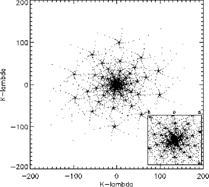
Figure 1: LOFAR instantaneous $(u,v)$ coverage for a declination $\delta_{0}=\pi/2$. The units on the $x$ and $y$ axis are Kilo-$\lambda$, where $\lambda$ is the mean band wavelength. The box on the lower right corner shows a zoom of the $(u,v)$ coverage between -5 and 5 Kilo-$\lambda$.

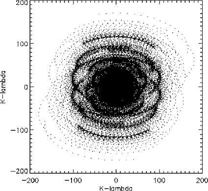
Figure 2: LOFAR $(u,v)$ coverage for $\delta_{0}=\pi/6$ declination angle after 8 hours integration time, with the same units as in Fig.1.

5.1 Synthetic radio maps

To produce synthetic radio maps of the reionization process as seen by LOFAR we proceed as follows. We denote by $l_{c}=20/128\;h^{-1}$ Mpc the comoving thickness of a slice of the simulation box, and with:

$$L_{c}\approx 1.7\left(\frac{\Delta\nu_{obs}}{0.1\mbox{MHz}}\right)\left(\frac{1+z}{10}\right)^{1/2}\left(\frac{\Omega_{m}h^{2}}{0.15}\right)^{-1/2}\;{\rm Mpc},$$ (9)

the comoving length corresponding to an observational bandwidth $\Delta\nu_{obs}$. The number of slices that corresponds to a fixed $\Delta\nu_{obs}$ is $n_{c}=L_{c}/l_{c}$. For a given $\Delta\nu_{obs}$, we extract from each simulation a 2D map of brightness temperature by averaging the values of $\delta T_{b}$ on a number of slices $n_{c}$.

The maps are first Fourier-transformed and then they are convolved with the $(u,\,v)$ coverage, $S(u,\,v)$, given in Eqs. 7-8 and shown in Fig. 2. Such convolution is necessary to take into account the limitations due to LOFAR’s sampling function. We assume a monochromatic $(u,\,v)$ coverage, i.e. we neglect the width of the tracks in the $(u,\,v)$ plane. This represents a simplification, however we find that for the present study this approximation has a small impact on the results in comparison to the sensitivity limits of the instrument, because of the exceptionally complete $(u,\,v)$ coverage due to the log-spiral arms configuration of LOFAR. Next, an inverse Fourier transform has been performed to return to the image plane including the estimated instrumental sensitivity on different scales and frequencies as given at the official LOFAR website . The sensitivity of an interferometer is $\propto(\Delta\nu_{obs}\Delta t)^{-1/2}$; we assumed an observational bandwidth $\Delta\nu_{obs}=128$ kHz and an observation time $\Delta t=1000$ hours. Finally, we have convolved the resulting image with a gaussian beam of $\approx 3$ arcmin. This choice represents the best compromise between LOFAR sensitivity (which decreases for smaller beams) and the size of the simulation box, which is limited to $\approx 11$ arcmin. On this angular scale LOFAR will likely be able to detect the 21 cm signal thanks to its large collecting area in the Virtual Core. We note that this is mathematically analogous to applying a taper in the $(u,\,v)$ plane to give greater weighting to data from the shorter baselines, which is entirely consistent with the most critical part of the data being collected by the Virtual Core.

The results of this procedure are presented in Fig. 3 for the S5 model, i.e. the late reionization scenario in which the EoR is located at $z\approx 8$, the most promising in terms of 21 cm line detection from the pre-reionization IGM. The maps represent the 21 cm emission brightness temperature in logarithmic scale, both directly from the numerical simulation (i.e. before the convolution with LOFAR instrumental characteristics) and in the synthetic LOFAR images; the calculations were performed using the simulation outputs at redshifts $z=$ 10.6, 9.89 and 9.26 (corresponding to $\nu=$ 122, 130 and 138 MHz respectively). We find a region that should be detectable at a 3-$\sigma$ level, showing that if reionization occurred relatively late LOFAR should detect the signal from the neutral IGM. The resolution and sensitivity of the instrument allow the identification not only of the largely neutral IGM, but also of the HII holes produced by the ionizing sources. The brightest emission peaks at $z=10.6$ have $\delta T_{b}=35$ mK (the corresponding value in the original simulated map is $\sim 0.2$ K), whereas the holes are typically a factor of 5 below that - a dynamical range large enough to allow their robust identification as LOFAR’s sensitivity will be $\sim 10$ mK at these scales, frequencies, observational bandwidth and integration time. Even more importantly, the three synthetic maps demonstrate that the 21 cm line tomography can provide a superb tool to track the redshift evolution of the reionization process (the accuracy of this measurement could be noticeably enhanced by cross-correlating the 21 cm emission with CMB secondary anisotropies, see Salvaterra et al. 2005).

We have repeated the same analysis halving (doubling) the observational bandwidth, i.e. $\Delta\nu_{obs}=64\,\,(256)$ kHz; this corresponds to a sensitivity decrease (increase) by a factor $\sqrt{2}$ with respect the case analyzed above. The brightest structures in the synthetic maps at $z=10.6$ have $\delta T_{b}=34$ mK for $\Delta\nu_{obs}=64$ kHz with a dynamical range of 28 mK. The worse sensitivity (14 mK) obtained for this bandwith results only in a 2-$\sigma$ detection. For the largest $\Delta\nu_{obs}=256$ kHz, instead the peak $\delta T_{b}=33$ mK, and the dynamical range is 21 mK. Hence, given a sensitivity of $\approx 7$ mK, this would represent a 3-$\sigma$ detection in analogy with the $\Delta\nu_{obs}=128$ kHz case. Thus, we conclude that using the median observational bandwidth is preferable as it allows to have a fine-grained IGM tomography without missing too much signal.

The situation is less promising in early reionization models as the L20 we have studied. In this case, the rapid disappearance of the neutral IGM component negatively affects the detection in two ways: (i) the instrumental sensitivity decreases rapidly at low frequencies (i.e. towards higher redshift); (ii) the sky brightness temperature increases drastically. In this case, for a $\Delta\nu_{obs}=128$ kHz (corresponding to a sensitivity of about 80 mK), we find a peak value $\delta T_{b}=56$ mK, a dynamic range of 26 mK. This corresponds to 0.32 $\sigma$, implying an extremely difficult detection of the neutral IGM in an early reionization scenario.

Thus we conclude that, although one cannot exclude that even early reionization scenarios may lead to a positive LOFAR detection, the most favorable case would be one in which the EoR took place relatively recently. If this is the case we have shown that in principle LOFAR will be able to see reionization in its full action.

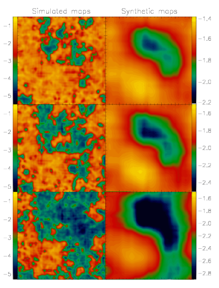
Figure 3: Logarithmic brightness temperature, $\log[\delta T_{b}/K]$, maps (linear size $\approx 11$ arcmin) of the 21 cm emission for the late reionization model S5 at redshifts $z=10.6,9.89,9.26$ from top to bottom, respectively. Left panels: maps obtained directly from the simulation, i.e. before convolution with LOFAR characteristics; Right: LOFAR synthetic maps.

6 Conclusions

By convolving simulations of cosmic reionization and 21 cm line emission with the provisional characteristics of the radio telescope LOFAR, we have shown that LOFAR has in principle the sensitivity to detect the signal from neutral hydrogen in the IGM, at least for a late reionization scenario (EoR at $z\approx 8$) that appears to be more appropriate after the release of the third year WMAP data analysis results. If reionization occurred earlier, the experiment is much more challenging. Nevertheless, even an upper limit on the neutral fraction at different epochs would represent a cornerstone result which could also strongly constrain more complex/double reionization histories. Our study is an attempt at making specific predictions for LOFAR based on state-of-the-art simulations, and it is affected by a number of limitations and approximations. Although our simulation box is one of the largest used so far in numerical reionization studies, the considered volume of (30 Mpc)³ is only marginally able to capture the global characteristics of cosmic reionization. Larger boxes could be used, but information on small scale structure (clumping) is easily smoothed out and lost, resulting in an extremely coarse description of the recombination processes. It is only very recently (Kohler, Gnedin & Hamilton 2005, Iliev et al. 2006) that dedicated investigations has started to tackle this very difficult problem.

It is beyond the scope of this paper also to deal with the crucial problems of ionospheric scintillation and foreground contamination (i.e. Galactic free-free and synchrotron emission, unresolved extra-galactic radio sources, free-free emission from ionizing sources, synchrotron emission from cluster radio halos and relics); rather, we consider the idealized condition in which the reionization signal is the only one present in the sky. A number of studies have discussed these complications in some detail (e.g. Shaver et al. 1999; Oh & Mack 2003; Di Matteo, Ciardi & Miniati 2004) and we refer the reader to those papers for more information. We note however, the success of the experiment will depend on the capability of effectively removing the foregrounds and of correcting for ionospheric variations (e.g. Gnedin & Shaver 2004; Zaldarriaga, Furlanetto & Hernquist 2004; Santos, Cooray & Knox 2005; Morales, Bowman & Hewitt 2005).

References

- [1] Bowman, J., Morales, M., Hewitt, J., 2005, astro-ph/0507357
- [2] Carilli, C., Gnedin, N. Y. & Owen, F. 2002, ApJ, 577, 22
- [3] Chen, X. & Miralda-Escudé, J. 2004, ApJ, 602, 1
- [4] Choudhury, T. R. & Ferrara, A. 2005, MNRAS, 361, 577
- [5] Ciardi, B., Ferrara, A., Marri, S. & Raimondo, G. 2001, MNRAS, 324, 381
- [6] Ciardi, B., Ferrara, A. & White, S.D.M. 2003, MNRAS, 344, L7 (CFW)
- [7] Ciardi, B. & Madau, P. 2003, ApJ, 596, 1
- [8] Ciardi, B., Stoehr, F. & White, S.D.M. 2003, MNRAS, 343, 1101
- [9] Ciardi B., Ferrara A., 2005, Space Sci. Rev., 116, 625
- [10] Di Matteo, T., Ciardi, B., Miniati, F., 2004, MNRAS, 355, 1053
- [11] Field, G. B. 1959, ApJ, 129, 551
- [12] Furlanetto, S. R., Sokasian, A., Hernquist, L., 2004, MNRAS, 347, 187
- [13] Furlanetto, S. R., Zaldarriaga, M., Hernquist, L., 2004, ApJ, 613, 16
- [14] Gallerani, S., Choudhury T. R. & Ferrara, A. 2005, MNRAS, submitted (astroph/0512129)
- [15] Gnedin, N. 2000, ApJ, 535, 530
- [16] Gnedin, N. 2004, ApJ, 610, 9
- [Gnedin & Shaver(2004)] Gnedin, N. Y., Shaver, P. A., 2004, ApJ, 608, 611
- [17] Hirata, C.M. 2005, ApJ, in press (astro-ph/0507102)
- [18] Iliev, I., Mellema, G., Pen, U., Merz, H., Shapiro, P. & Alvarez, M. 2006, MNRAS, submitted (astroph/0512187)
- [19] Kassim, N. E., Lazio, T. J. W., Ray, P. S., Crane, P. C., Hicks, B. C., Stewart, K. P., Cohen, A. S., & Lane, W. M. 2004, Planet. Space Sci., 52, 1343
- [20] Kauffmann, G., Colberg, J. M., Diaferio, A., & White, S. D. M. 1999, MNRAS, 303, 188
- [21] Kohler, K., Gnedin, N. Y. & Hamilton, A. J. S. 2005, astro-ph/0511627
- [22] Kogut, A. et al. 2003, ApJS, 148, 161
- [23] Madau, P., Meiksin, A., & Rees, M. J. 1997, ApJ, 475, 492
- [24] Maselli, A., Ferrara, A. & Ciardi, B. 2003, MNRAS, 345, 379
- [25] Morales, M. F., Bowman, J. D., Hewitt, J. N., 2005, ApJ submitted (astro-ph/0510027)
- [Oh & Mack(2003)] Oh, S. P., Mack, K. J., 2003, MNRAS, 346, 871
- [26] Pen, U. L.,Wu, X. P., Peterson, J. 2004, astro-ph/0404083
- [27] Salvaterra, R., Ciardi, B., Ferrara, A. & Baccigalupi, C. 2005, 2005, MNRAS, 360, 1063
- [28] Santos, M. G., Cooray, A., Knox, L., 2005, ApJ, 625, 575
- [Shaver et al.(1999)] Shaver, P., Windhorst, R., Madau, P., de Bruyn, G., 1999, A&A, 345, 380
- [29] Sokasian, A., Abel, T., Hernquist, L. E. & Springel, V. 2003, MNRAS, 344, 607
- [30] Spergel, D. N. et al., 2003, ApJS, 148, 175
- [31] Spergel, D. N. et al. 2006, astro-ph/0603449
- [32] Springel, V., White, S. D. M., Tormen, G., & Kauffmann, G. 2001, MNRAS, 328, 726
- [33] Springel, V., Yoshida, N., & White, S. D. M. 2001, NewA, 6, 79
- [34] Taylor, G. B., Carilli, C. L., & Perley, R. A., 1998, Synthesis Imaging in Radio Astronomy II: ASP Conf. Series Vol. 180, 211
- [35] Venkatesan, A., Giroux, M. L., & Shull, J. M. 2001, ApJ, 563, 1
- [36] White, R.L., Becker, R.H., Fan, X., Strauss, M.A., 2003, ApJ, 126, 1
- [37] Wyithe, J.S., Loeb, A., Barnes, D., 2005, astro-ph/0506045
- [38] Wouthuysen, S. A. 1952, AJ, 57, 31
- [39] Yoshida, N., Sheth, R. K., & Diaferio, A. 2001, MNRAS, 328, 669
- [Zaldarriaga, Furlanetto & Hernquist(2004)] Zaldarriaga, M., Furlanetto, S. R., Hernquist, L., 2004, ApJ, 608, 622