Effect of heat flux on differential rotation in turbulent convection

Abstract

We studied the effect of the turbulent heat flux on the Reynolds stresses in a rotating turbulent convection. To this end we solved a coupled system of dynamical equations which includes the equations for the Reynolds stresses, the entropy fluctuations and the turbulent heat flux. We used a spectral $\tau$ approximation in order to close the system of dynamical equations. We found that the ratio of the contributions to the Reynolds stresses caused by the turbulent heat flux and the anisotropic eddy viscosity is of the order of $\sim 10\,(L_{\rho}/l_{0})^{2}$, where $l_{0}$ is the maximum scale of turbulent motions and $L_{\rho}$ is the fluid density variation scale. This effect is crucial for the formation of the differential rotation and should be taken into account in the theories of the differential rotation of the Sun, stars and planets. In particular, we demonstrated that this effect may cause the differential rotation which is comparable with the typical solar differential rotation.

I Introduction

Solar and stellar magnetic fields are believed to originate in a dynamo, driven by the joint action of the mean hydrodynamic helicity of turbulent convection and differential rotation (see, e.g., M78 ; P79 ; KR80 ; ZRS83 ; BSR05 , and references therein). It was suggested in K63 that the differential rotation of the Sun is caused by an anisotropic eddy viscosity which was described phenomenologically in K63 ; L41 ; D85 ; RUD89 . Theory of the differential rotation based on the idea of the anisotropic eddy viscosity was developed in a number of papers (see, e.g., KRUD93 ; D93 ; KRUD05 , and references therein). However, there is an additional effect which can strongly modify the differential rotation. In particular, the direct effect of the turbulent heat flux on the Reynolds stresses in a rotating turbulent convection is crucial for formation of the differential rotation.

The effect of rotation on a hydrodynamic turbulence was studied in numerous papers (see, e.g., DS79 ; KRUD93 ). However, a relation to the turbulent convection was made in previous theories of the differential rotation only phenomenologically, using the equation

$$\langle{\bf u^{\prime}}^{2}\rangle\propto g\tau_{0}\langle u^{\prime}_{z}s^{\prime}\rangle\;,$$ (1)

which follows from the mixing-length theory. Here $\langle u^{\prime}_{z}s^{\prime}\rangle$ is the vertical turbulent heat flux, ${\bf u}^{\prime}$ and $s^{\prime}$ are fluctuations of fluid velocity and entropy, ${\bf g}$ is the acceleration of gravity and $\tau_{0}$ is the characteristic correlation time of turbulent velocity field. Equation (1) implies that the vertical turbulent heat flux plays a role of a stirring force for the turbulence. However, a more sophisticated approach implies a solution of a coupled system of dynamical equations which includes the equations for the Reynolds stresses $\langle u^{\prime}_{i}u^{\prime}_{j}\rangle$, the turbulent heat flux $\langle s^{\prime}\,u^{\prime}_{i}\rangle$ and the entropy fluctuations $\langle s^{\prime 2}\rangle$ in a rotating turbulent convection. The latter has not been taken into account in the previous theories of the differential rotation.

The goal of this study is to analyze the effect of the turbulent heat flux on the Reynolds stresses in a rotating turbulent convection and on formation of the differential rotation. We demonstrated that this effect is crucial for the formation of the differential rotation, and it should be taken into account in theories of the differential rotation of the Sun, stars and planets. In particular, we found that the ratio of the contributions to the Reynolds stresses caused by the turbulent heat flux and the anisotropic eddy viscosity is of the order of $\sim 10(L_{\rho}/l_{0})^{2}$ for $\Omega\,\tau_{0}\leq 1$, where $l_{0}$ is the maximum scale of turbulent motions (the integral scale of turbulence), $\Omega$ is the rotation rate, $L_{\rho}$ is the fluid density variation scale, i.e., $(\mbox{\boldmath$\nabla$}\rho_{0})/\rho_{0}=-L_{\rho}^{-1}\,{\bf e}$, $\,\,\rho_{0}$ is the fluid density and ${\bf e}$ is the unit vector in the direction of the fluid density inhomogeneity. The turbulent heat flux contribution to the Reynolds stresses changes its sign when the direction of the vertical turbulent heat flux changes. This is the key difference from previous theories of the differential rotation. The effect of the turbulent heat flux on the Reynolds stresses in a turbulent convection may cause the differential rotation which is comparable with the typical differential rotation of the Sun. The data of the solar differential rotation is obtained from surface observations of the solar angular velocity (see, e.g., HH70 ; SH84 ) and from helioseismology based on measurements of the frequency of $p$-mode oscillations (see, e.g., DH86 ; DG89 ; T90 ; SAB98 ).

The mechanism of the differential rotation that is associated with the effect of the turbulent heat flux on Reynolds stresses in a rotating turbulent convection is as follows. Let us split the total rotation of fluid into a constant component $\Omega$ (uniform rotation) and the differential rotation $\delta\Omega$. The uniform rotation causes the counter-rotation turbulent heat flux (i.e., the toroidal turbulent heat flux, $\langle s^{\prime}\,u^{\prime}_{\varphi}\rangle$, directed opposite to the background rotation $\Omega$). Therefore, there is a correlation of fluctuations of the entropy $s^{\prime}$ and the toroidal component of the velocity, $u^{\prime}_{\varphi}$. Here $r,\theta,\varphi$ are the spherical coordinates.

The counter-rotation turbulent heat flux is similar to the counter-wind turbulent heat flux (in the direction opposite to the mean wind) which is well-known in the atmospheric physics. The counter-rotation turbulent heat flux arises by the following reason. In turbulent convection an ascending fluid element has larger temperature then that of surrounding fluid and smaller toroidal fluid velocity, while a descending fluid element has smaller temperature and larger toroidal fluid velocity. This causes the turbulent heat flux in the direction opposite to the toroidal mean fluid flow (i.e., opposite to rotation). The counter-rotation turbulent heat flux is determined by Eq. (24) in Section III.

The entropy fluctuations cause fluctuations of the buoyancy force, and this results in increase fluctuations of the vertical and meridional components of the velocity which are correlated with the fluctuations of the toroidal component of the velocity. These produce the off-diagonal components of the Reynolds stress tensor, $\langle u^{\prime}_{r}u^{\prime}_{\varphi}\rangle$ and $\langle u^{\prime}_{\theta}u^{\prime}_{\varphi}\rangle$, and create the toroidal component of the effective force which causes formation of the differential rotation $\delta\Omega$ in turbulent convection.

This paper is organized as follows. In Section II we formulated the governing equations, the assumptions, the procedure of the derivation, and described the effect of the turbulent heat flux on the Reynolds stresses. In Section III we developed the theory of the differential rotation based on this effect. In Section IV we made estimates for the solar differential rotation. In Appendixes A and B we performed a detailed derivation of the effect of the turbulent heat flux on the Reynolds stresses in the rotating turbulent convection.

II Effect of the turbulent heat flux on the Reynolds stresses

In order to study the effect of the turbulent heat flux on the Reynolds stresses we considered turbulent convection with large Rayleigh and Reynolds numbers. We employed a mean field approach whereby the velocity, pressure and entropy are separated into the mean and fluctuating parts, where the fluctuating parts have zero mean values. The large-scale fluid motions are determined by the mean-field equations, which follow from the momentum and entropy equations for instantaneous fields by averaging over an ensemble of fluctuations. The mean-field equations are given by

$$\biggl{(}{\partial\over\partial t} + {\bf U}\cdot\mbox{\boldmath$\nabla$}\biggr{)}\,U_{i}=-{\nabla}_{i}\,\biggl{(}{P\over\rho_{0}}\biggr{)}-{\bf g}\,S+2\,{\bf U}\times{\bf\Omega}$$ (2)

$$- ({\nabla}_{j}+L_{\rho}^{-1}\,e_{j})\,\langle u^{\prime}_{i}\,u^{\prime}_{j}\rangle+{\bf f}_{\nu}({\bf U})\;,$$

$$\biggl{(}{\partial\over\partial t} + {\bf U}\cdot\mbox{\boldmath$\nabla$}\biggr{)}\,S=-({\nabla}_{j}+L_{\rho}^{-1}\,e_{j})\,\langle s\,u_{i}\rangle$$ (3)

$$- {1\over T_{0}}\,\mbox{\boldmath$\nabla$}\cdot{\bf F}_{\kappa}({\bf U},S)\;,$$

where Eq. (2) is written in the reference frame uniformly rotating with the angular velocity ${\bf\Omega}$. Here the mean fields ${\bf U}$, $\,P$, $\,T$ and $S$ are the fluid velocity, pressure, temperature and entropy, respectively, $\rho_{0}\,{\bf f}_{\nu}({\bf U})$ is the mean molecular viscous force, ${\bf F}_{\kappa}({\bf U},S)$ is the mean heat flux that is associated with the molecular thermal conductivity. The mean fluid velocity ${\bf U}$ for a low Mach number flows satisfies the equation ${\rm div}\,(\rho_{0}\,{\bf U})=0$. Equations (2) and (3) are written in the anelastic approximation, which is a combination of the Boussinesq approximation and the condition ${\rm div}\,(\rho_{0}\,{\bf U})=0$. The variables with the subscript $"0"$ correspond to the hydrostatic nearly isentropic basic reference state, i.e., $\mbox{\boldmath$\nabla$}P_{0}=\rho_{0}{\bf g}$ and ${\bf g}\cdot[(\gamma P_{0})^{-1}\mbox{\boldmath$\nabla$}P_{0}-\rho_{0}^{-1}\mbox{\boldmath$\nabla$}\rho_{0}]\approx 0$, where $\gamma$ is the ratio of specific heats. The turbulent convection is regarded as a small deviation from a well-mixed adiabatic reference state.

In order to get a closed system of the mean-field equations we have to determine the dependencies of the Reynolds stresses $\langle u^{\prime}_{i}(t,{\bf x})\,u^{\prime}_{j}(t,{\bf x})\rangle$ and the turbulent heat flux $\langle s^{\prime}(t,{\bf x})\,u^{\prime}_{i}(t,{\bf x})\rangle$ on the mean fields. To this end we used equations for fluctuations of velocity and entropy in a rotating turbulent convection, which are obtained by subtracting Eqs. (2) and (3) for the mean fields from the corresponding equations for the instantaneous fields. The equations for fluctuations of velocity and entropy are given by

$${\partial{\bf u}^{\prime}\over\partial t} = -({\bf U}\cdot\mbox{\boldmath$\nabla$}){\bf u}^{\prime}-({\bf u}^{\prime}\cdot\mbox{\boldmath$\nabla$}){\bf U}-\mbox{\boldmath$\nabla$}\biggl{(}{p^{\prime}\over\rho_{0}}\biggr{)}$$ (4)

$$-{\bf g}\,s^{\prime}+2{\bf u}^{\prime}\times{\bf\Omega}+{\bf U}^{N}\;,$$

$${\partial s^{\prime}\over\partial t} = -{\Omega_{b}^{2}\over g}({\bf u}^{\prime}\cdot{\bf e})-({\bf U}\cdot\mbox{\boldmath$\nabla$})s^{\prime}+S^{N}\;,$$ (5)

where $U^{N}=\langle({\bf u}^{\prime}\cdot\mbox{\boldmath$\nabla$}){\bf u}^{\prime}\rangle-({\bf u}^{\prime}\cdot\mbox{\boldmath$\nabla$}){\bf u}^{\prime}+{\bf f}_{\nu}({\bf u}^{\prime})$ and $S^{N}=\langle({\bf u}\cdot\mbox{\boldmath$\nabla$})s\rangle-({\bf u}\cdot\mbox{\boldmath$\nabla$})s-(1/T_{0})\,\mbox{\boldmath$\nabla$}\cdot{\bf F}_{\kappa}({\bf u}^{\prime},s^{\prime})$ are the nonlinear terms which include the molecular dissipative terms, $\Omega_{b}^{2}=-{\bf g}\cdot\mbox{\boldmath$\nabla$}S$ is the Brunt-Väisälä frequency, $p^{\prime}$ are fluctuations of fluid pressure and the fluid velocity fluctuations ${\bf u}^{\prime}$ satisfy the equation ${\rm div}\,(\rho_{0}\,{\bf u}^{\prime})=0$.

To study the rotating turbulent convection we performed the derivations which include the following steps: (i) using new variables for fluctuations of velocity ${\bf v}=\sqrt{\rho_{0}}\,{\bf u}^{\prime}$ and entropy $s=\sqrt{\rho_{0}}\,s^{\prime}$; (ii) derivation of the equations for the second moments $M^{(II)}$ of the velocity fluctuations $\langle v_{i}\,v_{j}\rangle$, the entropy fluctuations $\langle s^{2}\rangle$ and the turbulent heat flux $\langle v_{i}\,s\rangle$ in the ${\bf k}$ space; (iii) application of the spectral closure (see Eq. (6) below) and solution of the derived second-moment equations in the ${\bf k}$ space; (iv) returning to the physical space to obtain formulae for the Reynolds stresses and the turbulent heat fluxes as the functions of the rotation rate $\Omega$ (see for details, Appendix A).

The second-moment equations include the first-order spatial differential operators $\hat{\cal N}$ applied to the third-order moments $M^{(III)}$. A problem arises how to close the system, i.e., how to express the set of the third-order terms $\hat{\cal N}M^{(III)}$ through the lower moments $M^{(II)}$ (see, e.g., O70 ; MY75 ; Mc90 ). Various approximate methods have been proposed in order to solve it. A widely used spectral $\tau$ approximation (O70 ; PFL76 ; KRR90 ; RK04 ; BK04 ; BS05 ) postulates that the deviations of the third-moment terms, $\hat{\cal N}M^{(III)}({\bf k})$, from the contributions to these terms afforded by the background turbulent convection, $\hat{\cal N}M_{0}^{(III)}({\bf k})$, are expressed through the similar deviations of the second moments, $M^{(II)}({\bf k})-M_{0}^{(II)}({\bf k})$:

$$\hat{\cal N}M^{(III)}({\bf k}) - \hat{\cal N}M_{0}^{(III)}({\bf k})$$ (6)

$$= -{M^{(II)}({\bf k})-M_{0}^{(II)}({\bf k})\over\tau(k)}\;,$$

where $\tau(k)$ is the characteristic relaxation time, which can be identified with the correlation time of the turbulent velocity field. The background turbulent convection (which corresponds to a nonrotating and shear-free turbulent fluid flow), is determined by the budget equations and the general structure of the moments is obtained by symmetry reasoning. The above procedure (see Appendix A) yields formulae for the Reynolds stresses and the turbulent heat flux in the rotating turbulent convection. In particular, this allowed us to determine the effect of the turbulent heat flux on the Reynolds stresses.

The differential rotation in the axisymmetric fluid flow is determined by linearized Eq. (2) for the toroidal component $U_{\varphi}(r,\theta)\equiv r\,\sin\theta\,\delta\Omega$ of the mean velocity:

$$\rho_{0}\,{\partial U_{\varphi}\over\partial t} = {1\over r^{3}}{\partial\over\partial r}(r^{3}\sigma_{r\varphi})+{1\over r\sin^{2}\theta}{\partial\over\partial\theta}(\sin^{2}\theta\,\sigma_{\theta\varphi})$$ (7)

$$+2\,\rho_{0}\,({\bf U}{\bf\times}{\bf\Omega})_{\varphi}\;,$$

where the tensor $\sigma_{ij}=-\langle v_{i}\,v_{j}\rangle$ is determined by the Reynolds stress tensor. In particular,

$$\sigma_{r\varphi} \equiv -e_{j}^{\varphi}\,e_{i}^{r}\,\langle v_{i}\,v_{j}\rangle=\rho_{0}\,\nu_{{}_{T}}\,r\,{\partial\over\partial r}\biggl{(}{U_{\varphi}\over r}\biggr{)}$$ (8)

$$+\sigma_{r\varphi}^{F}+\sigma_{r\varphi}^{u}\;,$$

$$\sigma_{\theta\varphi} \equiv -e_{j}^{\varphi}\,e_{i}^{\theta}\,\langle v_{i}\,v_{j}\rangle=\rho_{0}\,\nu_{{}_{T}}\,{\sin\theta\over r}\,{\partial\over\partial\theta}\biggl{(}{U_{\varphi}\over\sin\theta}\biggr{)}$$ (9)

$$+\sigma_{\theta\varphi}^{F}+\sigma_{\theta\varphi}^{u}\;,$$

where ${\bf e}^{r}$, $\,{\bf e}^{\theta}$ and $\,{\bf e}^{\varphi}$ are the unit vectors along the radial, meridional and toroidal directions of the spherical coordinates $r,\theta,\varphi$. There are three contributions to the tensor $\sigma_{ij}=-\langle v_{i}\,v_{j}\rangle$. In particular, the first term in the right hand side of Eqs. (8) and  (9) describes the isotropic turbulent viscosity $\propto\nu_{{}_{T}}$, the second term in Eqs. (8) and  (9) determines the contribution $\mbox{\boldmath$\sigma$}^{F}$ to the Reynolds stresses caused by the turbulent heat flux, and the third term in Eqs. (8) and  (9) determines the contribution $\mbox{\boldmath$\sigma$}^{u}$ to the Reynolds stresses caused by the anisotropy of turbulence due to the nonuniform fluid density and uniform rotation.

In Eq. (7) we neglected small molecular viscosity term and we took into account that in the axisymmetric fluid flow $\partial({\bf U},S)/\partial\varphi=0$ and $\delta\Omega/\Omega$ is a small parameter. We assumed that the toroidal component of the mean velocity is much larger than the poloidal component. This is typical for the solar and stellar convective zones. We also took into account that the fluid density is nonuniform in the radial direction. The first two terms in the right hand side of Eq. (7) are the $\varphi$ component of the divergence of the tensor $\sigma_{ij}$ written for the axisymmetric fluid flow in spherical coordinates. This is a standard form of the $\varphi$ component of the divergence of a tensor in spherical coordinates (see, e.g., BSL02 ).

Let us discuss the contribution, $\mbox{\boldmath$\sigma$}^{F}$, to the Reynolds stress tensor caused by the turbulent heat flux. The components of this tensor, $\sigma_{r\varphi}^{F}\equiv-e_{j}^{\varphi}\,e_{i}^{r}\,\langle v_{i}\,v_{j}\rangle^{F}$ and $\sigma_{\theta\varphi}^{F}=-e_{j}^{\varphi}\,e_{i}^{\theta}\,\langle v_{i}\,v_{j}\rangle^{F}$, were determined in Appendix A. They are given by

$$\sigma_{r\varphi}^{F} = {1\over 6}\,\rho_{0}\,\tau_{0}^{2}\,g\,F_{\ast}\,\Omega\,\sin\theta\,[\Phi_{1}(\omega)+\cos^{2}\theta\,\Phi_{2}(\omega)]\;,$$

$$\sigma_{\theta\varphi}^{F} = {1\over 3}\,\rho_{0}\,\tau_{0}^{2}\,g\,F_{\ast}\,\Omega\,\sin^{2}\theta\,\cos\theta\,\Phi_{2}(\omega)\;,$$ (11)

where the tensor $\langle v_{i}\,v_{j}\rangle^{F}$ determines the contribution to the Reynolds stresses which vanishes when $\langle s^{\prime}\,u^{\prime}_{z}\rangle\to 0$ (see Eq. (48) in Appendix A). Here $F_{\ast}=\langle s^{\prime}\,u^{\prime}_{z}\rangle$ is the vertical turbulent heat flux, the parameter $\omega=8\,\Omega\,\tau_{0}$, $\,\tau_{0}=l_{0}/u_{0}$ is the characteristic correlation time of turbulent velocity field, and $u_{0}$ is the characteristic turbulent velocity in the maximum scale of turbulent motions $l_{0}$. The functions $\Phi_{1}(\omega)$ and $\Phi_{2}(\omega)$ are shown in Fig. 1. The formulae for the functions $\Phi_{1}(\omega)$ and $\Phi_{2}(\omega)$ are given by Eqs. (52) and (53) in Appendix A. The asymptotic formulas for $\sigma_{r\varphi}^{F}$ and $\sigma_{\theta\varphi}^{F}$ for a slow rotation, $8\,\tau_{0}\,\Omega\ll 1$, are given by

$$\sigma_{r\varphi}^{F} \approx \rho_{0}\,\tau_{0}^{2}\,g\,F_{\ast}\,\Omega\,\sin\theta\;,$$

$$\sigma_{\theta\varphi}^{F} \approx 4\,\rho_{0}\,\tau_{0}^{4}\,g\,F_{\ast}\,\Omega^{3}\,\sin^{2}\theta\,\cos\theta\;,$$

and for $8\,\tau_{0}\,\Omega\gg 1$ they are given by

$$\sigma_{r\varphi}^{F} \approx {1\over 4\,\Omega}\,\rho_{0}\,g\,F_{\ast}\,\sin^{3}\theta\;,$$

$$\sigma_{\theta\varphi}^{F} \approx {1\over 2\,\Omega}\,\rho_{0}\,g\,F_{\ast}\,\sin^{2}\theta\,\cos\theta\;.$$

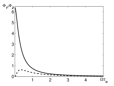
Figure 1: The functions $\Phi_{1}(\Omega\,\tau_{0})$ (solid) and $\Phi_{2}(\Omega\,\tau_{0})$ (dashed).

The contribution to the Reynolds stresses, $\mbox{\boldmath$\sigma$}^{u}$, in Eqs. (8) and (9) is caused by the anisotropy of turbulence due to the inhomogeneous fluid density and uniform rotation. The tensor $\mbox{\boldmath$\sigma$}^{u}$ determines the anisotropic eddy viscosity tensor with the nonzero off-diagonal components which are given by

$$\sigma_{r\varphi}^{u} \approx {l_{0}^{2}\over 15L_{\rho}^{2}}\,(\rho_{0}\,u_{0}^{2})\,\,(\Omega\,\tau_{0})\,\,\sin\theta\,[a_{1}(\Omega)-a_{2}(\Omega)\,\cos^{2}\theta]\;,$$

$$\sigma_{\theta\varphi}^{u} \approx {l_{0}^{2}\over 15L_{\rho}^{2}}\,(\rho_{0}\,u_{0}^{2})\,\,(\Omega\,\tau_{0})\,\,a_{2}(\Omega)\,\sin^{2}\theta\,\cos\theta\;,$$ (13)

(see, e.g., KRUD93 ), where $a_{1}(\Omega)\sim-1$ and $a_{2}(\Omega)\sim 2(\Omega\,\tau_{0})^{2}$ for $\Omega\,\tau_{0}\ll 1$, and $a_{1}(\Omega)\sim O[(\Omega\,\tau_{0})^{-3}]$ and $a_{2}(\Omega)\sim-(\Omega\,\tau_{0})^{-1}$ for $\Omega\,\tau_{0}\gg 1$. The contribution to the Reynolds stresses, $\mbox{\boldmath$\sigma$}^{u}$, due to the anisotropic eddy viscosity is smaller than that of $\mbox{\boldmath$\sigma$}^{F}$ due to the turbulent heat flux. In particular, the ratio $|{\sigma}^{F}/{\sigma}^{u}|\sim 10\,(L_{\rho}/l_{0})^{2}$ for $\Omega\,\tau_{0}\leq 1$. Note that for fast rotation rates $(\Omega\,\tau_{0}\gg 1)$ the validity of Eqs. (LABEL:A9) and (13) is questionable, because the quasi-linear approximation used in KRUD93 does not valid for $\Omega\,\tau_{0}\gg 1$.

For large Rayleigh numbers the contributions of anisotropies decrease in small scales. On the other hand, the rotation introduces an anisotropy in the turbulent convection. This causes non-zero off-diagonal components of the Reynolds stress tensor (see Eqs. (LABEL:B24)-(13)) and results in the redistribution of the turbulent heat flux on the surface of the rotating body (see Eq. (LABEL:B30)). Note that the main contribution to the tensor $\sigma_{ij}$ is at the maximum scale of turbulent motions. Therefore, the contributions to the tensor $\sigma_{ij}$ which depend on the Reynolds number are negligibly small. In the present study we investigated the large-scale effects (the differential rotation), and the influence of the molecular viscosity and molecular thermal diffusivity on the large-scale dynamics is very small in comparison with that of the eddy viscosity and turbulent thermal diffusivity. Therefore, the contributions to the tensor $\sigma_{ij}$ which depend on the molecular Prandtl number are also negligibly small.

III Differential rotation

In the present study for simplicity we have taken into account only the effect of $\mbox{\boldmath$\sigma$}^{F}$ on the differential rotation. Let us neglect the toroidal component of the Coriolis force in Eq. (7). This is valid when the poloidal components of the mean fluid velocity $U_{\theta}$ and $U_{r}$ are much smaller than $u_{0}\,l_{0}/L_{\rho}.$ This condition implies that the last term in the right hand side of Eq. (7) is much smaller than other terms. Here we took into account that $\sigma_{r\varphi}^{F}\propto\rho_{0}$ and the fluid density stratification length $L_{\rho}$ is much smaller than the solar radius $R_{\odot}$. Therefore, we neglected the effect of the meridional circulations on the differential rotation, which was studied in KRUD05 , among the others. For simplicity we also did not take into account the dependence of the turbulent viscosity on the rate of rotation. After these simplifications, Eq. (7) in dimensionless form reads

$$\biggl{[}{\partial\over\partial t}+{\hat{\cal M}(X)\over r^{2}}-\hat{\cal W}(r)\biggr{]}{\delta\Omega\over\Omega}={{\cal I}\over r^{2}}\;,$$ (14)

where

$$\hat{\cal M}(X) = (X^{2}-1){\partial^{2}\over\partial X^{2}}+4X{\partial\over\partial X}\;,$$

$$\hat{\cal W}(r) = {1\over\rho_{0}(r)\,r^{4}}\,{\partial\over\partial r}\biggl{(}\rho_{0}(r)\,r^{4}\,{\partial\over\partial r}\biggr{)}\;,$$

$${\cal I}(r) = I_{0}\,[\,(3-r\,\Lambda)\,\Phi_{1}(\omega)-2\,\Phi_{2}(\omega)$$

$$+\,\,(13-r\,\Lambda)\,\Phi_{2}(\omega)\,X^{2}\,]\;,$$

$I_{0}=\tau_{0}^{2}\,g\,F_{\ast}/6\,\nu_{{}_{T}}$, $\,\Lambda=R_{\odot}/L_{\rho}$ and $X=\cos\theta$. Here length is measured in units of the solar radius $R_{\odot}$ and time is measured in units of $R_{\odot}^{2}/\nu_{{}_{T}}$ based on the solar radius and the turbulent viscosity $\nu_{{}_{T}}$.

Solution of Eq. (14) we seek for in the form:

$${\delta\Omega\over\Omega}=\tilde{A}+{1\over\sqrt{\rho_{0}}}\sum_{n=0}^{\infty}\,C_{2n}^{3/2}(X)\sum_{m=3}^{\infty}\,V_{m,2n}(r)\,Q_{m,2n}(t)\;,$$

(15)

where the function $C_{n}^{3/2}(X)$ satisfies the equation for the ultra-spherical polynomials:

$$[\hat{\cal M}(X)-n(n+3)]\,C_{n}^{3/2}(X)=0\;.$$ (16)

The functions $V_{m,n}(r)$ in Eq. (15) are determined by equation of the eigenvalue problem

$$[\hat{\cal L}_{n}(r) - \gamma_{m}]\,V_{m,n}(r)=0\;,$$ (17)

with

$$\hat{\cal L}_{n}(r) = {d^{2}\over dr^{2}}+{4\over r}\,{d\over dr}+{2\Lambda\over r}-{\Lambda^{2}\over 4}-{n(n+3)\over r^{2}}\;.$$

The constant $\tilde{A}$ in Eq. (15) is determined from the conservation law for the total angular momentum $L_{\odot}\equiv\int\{{\bf r}{\bf\times}[(\Omega+\delta\Omega){\bf\times}{\bf r}]\}\,\rho_{0}({\bf r})\,d{\bf r}$ of the rotating body (e.g., the Sun). The functions $Q_{m,2n}(t)$ in Eq. (14) are determined in Appendix B. They are given by Eqs. (LABEL:C15)-(60).

Equation (17) coincides with the equation for the Kepler problem in quantum mechanics (the hydrogen atom in a spherically symmetric potential, see, e.g., F71 ). The solution of Eq. (17) is given by

$$V_{m,n}(r)=r^{n}\,\exp(-r\,\Lambda/m)\,\tilde{F}(a;\,b;\,2r\,\Lambda/m)\;,$$ (18)

where $\tilde{F}(a;\,b;\,y)$ is the confluent hypergeometric function with $a=n-m+2$ and $b=2(n+2)$. Here we assumed for simplicity that $L_{\rho}$ is independent of the radius. The characteristic spatial scale of the mean fields variations is of the order of the solar radius $R_{\odot}$ in the main part of the convective zone (except for its boundaries). On the other hand, the fluid density in the solar convective zone changes very strongly (in 6 - 7 orders of magnitude). Therefore, in the main part of the solar convective zone $r\,\Lambda\gg 1$, and Eq. (18) for the eigenfunctions $V_{m,n}(r)$ reduces to

$$V_{m,n}(r)=A\,r^{m-2}\,\exp(-r\,\Lambda/m)\;,$$ (19)

where the eigenvalues $\gamma_{m}$ are given by

$$\gamma_{m}=-{\Lambda^{2}(m^{2}-4)\over 4m^{2}}\,\;,$$ (20)

with the integer numbers $m\geq 3$. Here $\gamma_{m}$ is measured in units of $\nu_{{}_{T}}/R_{\odot}^{2}$. The constant $A$ in Eq. (19) is determined from the condition $\int_{r_{b}}^{1}\,r^{4}\,V_{m,n}^{2}(r)\,dr=1$, where $r_{b}=R_{b}/R_{\odot}$, $\,R_{b}$ is the radius of the bottom of the convective zone, and $r=R/R_{\odot}$ is the dimensionless radius measured in units of the solar radius $R_{\odot}$. Therefore, the differential rotation caused by the effect of the turbulent heat flux on the Reynolds stresses in a turbulent convection is determined by the following equation:

$${\delta\Omega\over\Omega} = {L_{\rho}\over R_{\odot}}\,\biggl{[}{\tau_{0}^{2}\,g\,F_{\ast}\over\nu_{{}_{T}}}\biggr{]}\,\sum_{m=3}^{\infty}\,\biggl{\{}\beta_{m}\,\biggl{[}{\rho_{0}(R_{b})\over\rho_{0}(R_{\odot})}\biggr{]}^{m-2\over 2m}$$ (21)

$$-\biggl{(}{R\over R_{\odot}}\biggr{)}^{m-2}\,\biggl{[}{\rho_{0}(R_{b})\over\rho_{0}(R)}\biggr{]}^{m-2\over 2m}\,[f_{1,m}(\omega)$$

$$+f_{2,m}(\omega)\,\cos^{2}\theta]\biggr{\}}\;,$$

where

$$f_{1,m}(\omega) = K(m)\,\biggl{[}\tilde{\Phi}_{1}(\omega)-3K_{\ast}(m)\,{L_{\rho}\over R_{\odot}}\,\tilde{\Phi}_{2}(\omega)\biggr{]}\;,$$

$$f_{2,m}(\omega) = K(m)\,\Phi_{2}(\omega)\biggl{[}1-13K_{\ast}(m)\,{L_{\rho}\over R_{\odot}}\biggr{]}\;,$$

$$\beta_{m} = {L_{\rho}\over R_{\odot}}\,\biggl{(}{10\,m\over m-2}\biggr{)}\,\biggl{[}{f_{1}+f_{2}/5\over 1-(R_{b}/R_{\odot})^{5}}\biggr{]}\;,$$

$K(m)=8m^{2}/[3(m^{2}-4)(m+2)]$, $\,\tilde{\Phi}_{1}(\omega)=\Phi_{1}(\omega)+(13/10)\Phi_{2}(\omega)$ and $\,\tilde{\Phi}_{2}(\omega)=\Phi_{1}(\omega)+5\Phi_{2}(\omega)$, the parameter $K_{\ast}(m)$ is given by Eq. (61) in Appendix B. In the next section we use Eq. (21) in order to estimate the solar differential rotation.

IV Discussion

The effect of the turbulent heat flux on the Reynolds stresses in a turbulent convection may cause the differential rotation comparable with the typical differential rotation of the Sun. Indeed, let us use estimates of governing parameters taken from models of the solar convective zone, e.g., S74 ; BT66 . More modern treatments make little difference to these estimates. In particular, at depth of the convective zone, $H\sim 10^{10}$ cm measured from the top (i.e., at $R=0.85R_{\odot}$), the parameters are: the maximum scale of turbulent motions $l_{0}\sim 5.5\times 10^{9}$ cm; the characteristic turbulent velocity in the maximum scale of turbulent motions $u_{0}\sim 5.4\times 10^{3}$ cm s^-1; the turbulent viscosity $\nu_{{}_{T}}\sim 10^{13}$ cm² s^-1; the fluid density $\rho_{0}\sim 7.6\times 10^{-2}$ g cm^-3 and the fluid density stratification length $L_{\rho}\sim 10^{10}$ cm. Thus, Eq. (21) yields the following estimates for the solar differential rotation

$$\left|{\partial\over\partial r}\delta\Omega\right| \approx 200\,(1+0.4\,\cos^{2}\theta)\,{nHz\over R_{\odot}}\;,$$ (22)

$${1\over r}\,\left|{\partial\over\partial\theta}\delta\Omega\right| \approx 140\,\sin(2\theta)\,{nHz\over R_{\odot}}\;.$$ (23)

These estimates are in agreement with the data obtained from surface observations of the solar angular velocity HH70 ; SH84 and from helioseismology DH86 ; DG89 ; T90 ; SAB98 . Therefore, the effect of the turbulent heat flux on the Reynolds stresses in a turbulent convection is crucial for the formation of the differential rotation and should be taken into account in theories of the differential rotations of the Sun and solar-like stars.

The mechanism of the differential rotation due to the effect of the turbulent heat flux on the Reynolds stresses, is related to the counter-rotation turbulent heat flux in turbulent convection. This flux reads:

$${\bf F}^{\rm CR} = -{3\,F_{\ast}\over 8\,\omega}\,\biggl{[}2\,\biggl{(}{\arctan\,\omega\over\omega}-1\biggr{)}$$ (24)

$$+\;\;\ln(1+\omega^{2})\biggr{]}\,\sin\,\theta\,{\bf e}_{\varphi}\;,$$

[see Eq. (LABEL:B30)]. Therefore, the entropy fluctuations correlate with the toroidal component of the velocity. The entropy fluctuations result in fluctuations of the buoyancy force, that increases fluctuations of the poloidal components of the velocity (which are correlated with the fluctuations of the toroidal component of the velocity). These produce the off-diagonal components of the Reynolds stress tensor which cause the formation of the differential rotation.

Appendix A The Reynolds Stresses in rotating turbulent convection

We use a mean field approach whereby the velocity, pressure and entropy are separated into the mean and fluctuating parts, where the equations in the new variables for fluctuations of velocity ${\bf v}=\sqrt{\rho_{0}}\,{\bf u}^{\prime}$ and entropy $s=\sqrt{\rho_{0}}\,s^{\prime}$ follow from Eqs. (4) and (5):

$${1\over\sqrt{\rho_{0}}}{\partial{\bf v}({\bf x},t)\over\partial t} = -\mbox{\boldmath$\nabla$}\biggl{(}{p^{\prime}\over\rho_{0}}\biggr{)}+{1\over\sqrt{\rho_{0}}}\biggl{[}2{\bf v}\times{\bf\Omega}-({\bf v}\cdot\mbox{\boldmath$\nabla$}){\bf U}$$ (25)

$$- G^{U}\,{\bf v}-{\bf g}\,s\biggr{]}+{\bf F}_{M}+{\bf v}^{N}\;,$$

$${\partial s({\bf x},t)\over\partial t} = -{\Omega_{b}^{2}\over g}({\bf v}\cdot{\bf e})-G^{U}\,s+s^{N}\;,$$ (26)

where $G^{U}=(1/2)\,{\rm div}\,{\bf U}+{\bf U}{\bf\cdot}\mbox{\boldmath$\nabla$}$, $\,{\bf v}^{N}$ and $s^{N}$ are the nonlinear terms which include the molecular viscous and dissipative terms, $p^{\prime}$ are fluctuations of fluid pressure. The fluid velocity fluctuations ${\bf v}$ satisfy the equation $\mbox{\boldmath$\nabla$}\cdot{\bf v}=(1/2\,L_{\rho})({\bf v}\cdot{\bf e})$, where $(\mbox{\boldmath$\nabla$}\rho_{0})/\rho_{0}=-L_{\rho}^{-1}\,{\bf e}.$ Equations (25) and (26) are written in the anelastic approximation. The variables with the subscript $"0"$ correspond to the hydrostatic nearly isentropic basic reference state. The turbulent convection is regarded as a small deviation from a well-mixed adiabatic reference state.

Let us derive equations for the second-order moments. For this purpose we rewrite the momentum equation and the entropy equation in a Fourier space. In particular,

$${dv_{i}({\bf k})\over dt} = [D_{im}^{\Omega}({\bf k})+I_{im}^{U}({\bf k})]v_{m}({\bf k})+g\,e_{m}\,P_{im}({\bf k})\,s({\bf k})$$ (27)

$$+v_{i}^{N}({\bf k})\;,$$

$${ds({\bf k})\over dt} = -G^{U}({\bf k})\,s({\bf k})+s^{N}\;.$$ (28)

To derive Eq. (27) we multiplied the momentum equation written in ${\bf k}$-space by $P_{ij}({\bf k})=\delta_{ij}-k_{ij}$ in order to exclude the pressure term from the equation of motion. Here

$$I_{ij}^{U}({\bf k}) = 2k_{in}\nabla_{j}U_{n}-\nabla_{j}U_{i}-G^{U}({\bf k})\delta_{ij}\;,$$

$$G^{U}({\bf k}) = {1\over 2}\,{\rm div}\,{\bf U}+i({\bf U}{\bf\cdot}{\bf k})\;,$$

$$D_{ij}^{\Omega}({\bf k}) = 2\varepsilon_{ijm}\Omega_{n}k_{mn}\;,$$

and $\delta_{ij}$ is the Kronecker tensor, $k_{ij}=k_{i}k_{j}/k^{2}$ and $\varepsilon_{ijk}$ is the Levi-Civita tensor. Using Eqs. (27)-(28) we derive equations for the following correlation functions:

$$f_{ij}({\bf k}) = \hat{L}(v_{i};v_{j})\;,\;\;F_{i}({\bf k})=\hat{L}(s;v_{i})\;,$$

$$\Theta_{i}({\bf k}) = \hat{L}(s;s)\;,$$

where

$$\hat{L}(a;c)=\int\langle a(t,{\bf k}+{\bf K}/2)c(t,-{\bf k}+{\bf K}/2)\rangle$$

$$\times\exp{(i{\bf K}{\bf\cdot}{\bf R})}\,d{\bf K}\;,$$

${\bf R}$ and ${\bf K}$ correspond to the large scales, and ${\bf r}$ and ${\bf k}$ to the small ones. Hereafter we omitted argument $t$ and ${\bf R}$ in the correlation functions. The equations for these correlation functions are given by

$${\partial f_{ij}({\bf k})\over\partial t} = (I_{ijmn}^{U}+D_{ijmn}^{\Omega})f_{mn}+M_{ij}^{F}+\hat{\cal N}\tilde{f}_{ij},$$ (29)

$${\partial F_{i}({\bf k})\over\partial t} = (I_{im}^{U}+D_{im}^{\Omega})F_{m}+ge_{m}P_{im}(k)\Theta({\bf k})+\hat{\cal N}\tilde{F}_{i}\;,$$

$${\partial\Theta({\bf k})\over\partial t} = -{\rm div}\,[{\bf U}\,\Theta({\bf k})]+\hat{\cal N}\Theta\;,$$ (31)

where

$$I_{ijmn}^{U} = I^{U}_{im}({\bf k}_{1})\,\delta_{jn}+I^{U}_{jm}({\bf k}_{2})\,\delta_{in}$$ (32)

$$= \biggl{[}2k_{iq}\delta_{mp}\delta_{jn}+2k_{jq}\delta_{im}\delta_{pn}-\delta_{im}\delta_{jq}\delta_{np}$$

$$\;-\delta_{iq}\delta_{jn}\delta_{mp}+\delta_{im}\delta_{jn}k_{q}{\partial\over\partial k_{p}}\biggr{]}\nabla_{p}U_{q}$$

$$\;-\delta_{im}\delta_{jn}\,[{\rm div}\,{\bf U}+{\bf U}{\bf\cdot}\mbox{\boldmath$\nabla$}]\;,$$

$$D_{ijmn}^{\Omega} = D_{im}^{\Omega}({\bf k}_{1})\,\delta_{jn}+D_{jm}^{\Omega}({\bf k}_{2})\,\delta_{in}$$ (33)

$$= 2\,\Omega_{q}k_{pq}(\varepsilon_{imp}\,\delta_{jn}+\varepsilon_{jmp}\,\delta_{in})\;,$$

$$M_{ij}^{F} = ge_{m}[P_{im}({\bf k})F_{j}({\bf k})+P_{jm}({\bf k})F_{i}(-{\bf k})],$$ (34)

and ${\bf k}_{1}={\bf k}+{\bf K}/2$, $\,{\bf k}_{2}=-{\bf k}+{\bf K}/2$. Note that the correlation functions $f_{ij}$, $\,F_{i}$ and $\Theta$ are proportional to the fluid density $\rho_{0}({\bf R})$. Here $\hat{\cal N}\tilde{f}_{ij}$, $\,\hat{\cal N}\tilde{F}_{i}$ and $\hat{\cal N}\Theta$ are the terms which are related to the third-order moments appearing due to the nonlinear terms. In particular,

$$\hat{\cal N}\tilde{f}_{ij} = \langle P_{im}({\bf k}_{1})v^{N}_{m}({\bf k}_{1})v_{j}({\bf k}_{2})\rangle$$

$$+\langle v_{i}({\bf k}_{1})P_{jm}({\bf k}_{2})v^{N}_{m}({\bf k}_{2})\rangle\;,$$

$$\hat{\cal N}\tilde{F}_{i} = \langle s^{N}({\bf k}_{1})u_{j}({\bf k}_{2})\rangle+\langle s({\bf k}_{1})P_{im}({\bf k}_{2})v^{N}_{m}({\bf k}_{2})\rangle\;,$$

$$\hat{\cal N}\Theta = \langle s^{N}({\bf k}_{1})s({\bf k}_{2})\rangle+\langle s({\bf k}_{1})s^{N}({\bf k}_{2})\rangle\;.$$

When div $\,{\bf U}=0$, Eq. (32) coincides with that derived in EKRZ02 .

The equations for the second-order moments contain high-order moments and a closure problem arises (see, e.g., O70 ; MY75 ; Mc90 ). We apply the spectral $\tau$ approximation (or the third-order closure procedure, see, e.g., O70 ; PFL76 ; KRR90 ; RK04 ; BK04 ; BS05 ). The spectral $\tau$ approximation postulates that the deviations of the third-order-moment terms, $\hat{\cal N}f_{ij}({\bf k})$, from the contributions to these terms afforded by the background turbulent convection, $\hat{\cal N}f_{ij}^{(0)}({\bf k})$, are expressed through the similar deviations of the second moments, $f_{ij}({\bf k})-f_{ij}^{(0)}({\bf k})$, i.e.,

$$\hat{\cal N}f_{ij}({\bf k})-\hat{\cal N}f_{ij}^{(0)}({\bf k})=-{f_{ij}({\bf k})-f_{ij}^{(0)}({\bf k})\over\tau(k)}\;,$$ (35)

and similarly for other tensors, where $\hat{\cal N}f_{ij}=\hat{\cal N}\tilde{f}_{ij}+M_{ij}^{F}(F^{\Omega=0})$ and $\hat{\cal N}F_{i}=\hat{\cal N}\tilde{F}_{i}+ge_{n}P_{in}(k)\Theta^{\Omega=0}$, the superscript $(0)$ corresponds to the background turbulent convection (i.e., a nonrotating turbulent convection with $\nabla_{i}\bar{U}_{j}=0)$, $\,\tau(k)$ is the characteristic relaxation time of the statistical moments. The quantities $F^{\Omega=0}$ and $\Theta^{\Omega=0}$ are for a nonrotating turbulent convection with nonzero spatial derivatives of the mean velocity. Note that we applied the $\tau$-approximation (35) only to study the deviations from the background turbulent convection which are caused by the spatial derivatives of the mean velocity and a nonzero rotation. The background turbulent convection is assumed to be known (see below).

Solution of Eqs. (29)-(31) after applying the spectral $\tau$ approximation reads

$$f_{ij}({\bf k}) = f^{(0)}_{ij}({\bf k})+f^{F}_{ij}({\bf k})+f^{U}_{ij}({\bf k})\;,$$ (36)

$$F_{i}({\bf k}) = \tilde{D}_{im}^{-1}({\bf\Omega})F^{(0)}_{m}({\bf k})\;,$$ (37)

$$\Theta({\bf k}) = [1-\tau({\bf U}{\bf\cdot}\mbox{\boldmath$\nabla$})]\Theta^{(0)}({\bf k})\;,$$ (38)

where

$$f^{U}_{ij}({\bf k}) = \tau\tilde{D}_{ijmn}^{-1}({\bf\Omega})I_{mnpq}^{U}[f^{(0)}_{pq}+f^{F}_{pq}]\;,$$ (39)

$$f^{F}_{ij}({\bf k}) = \tau\tilde{D}_{ijmn}^{-1}({\bf\Omega})\tilde{M}_{mn}^{F}({\bf k})\;,$$ (40)

$$\tilde{M}_{ij}^{F}({\bf k}) = ge_{m}\{P_{im}({\bf k})[F_{j}({\bf k})-F_{j}^{\Omega=0}({\bf k})]$$ (41)

$$+P_{jm}({\bf k})[F_{i}(-{\bf k})-F_{i}^{\Omega=0}(-{\bf k})]\}.$$

Here $\tilde{D}_{ij}^{-1}({\bf\Omega})$ is the inverse of $\tilde{D}_{ij}({\bf\Omega})=\delta_{ij}-\tau D_{ij}^{\Omega}$ and $\tilde{D}_{ijmn}^{-1}({\bf\Omega})$ is the inverse of $\tilde{D}_{ijmn}({\bf\Omega})=\delta_{im}\delta_{jn}-\tau\,D_{ijmn}^{\Omega}$, and

$$\tilde{D}_{ij}^{-1}({\bf\Omega})=\chi(\psi)\,(\delta_{ij}+\psi\,\varepsilon_{ijm}\,\hat{k}_{m}+\psi^{2}\,k_{ij})\;,$$ (42)

$$\tilde{D}_{ijmn}^{-1}({\bf\Omega})={1\over 2}[B_{1}\,\delta_{im}\delta_{jn}+B_{2}\,k_{ijmn}+B_{3}\,(\varepsilon_{ipm}\delta_{jn}$$

$$+\varepsilon_{jpn}\delta_{im})\hat{k}_{p}+B_{4}\,(\delta_{im}k_{jn}+\delta_{jn}k_{im})$$

$$+B_{5}\,\varepsilon_{ipm}\varepsilon_{jqn}k_{pq}+B_{6}\,(\varepsilon_{ipm}k_{jpn}+\varepsilon_{jpn}k_{ipm})]\;,$$ (43)

and $\hat{k}_{i}=k_{i}/k$, $\,\chi(\psi)=1/(1+\psi^{2})$, $\,\psi=2\tau(k)\,({\bf k}\cdot{\bf\Omega})/k$, $\,B_{1}=1+\chi(2\psi),$ $\,B_{2}=B_{1}+2-4\chi(\psi),$ $\,B_{3}=2\psi\,\chi(2\psi),$ $\,B_{4}=2\chi(\psi)-B_{1},$ $\,B_{5}=2-B_{1}$ and $B_{6}=2\psi\,[\chi(\psi)-\chi(2\psi)]$. For derivation of Eqs. (36) and (39)-(40) we used a procedure described in Appendix B in EGKR05 .

For the integration in ${\bf k}$-space of the second moments $f_{ij}({\bf k})$, $\,F_{i}({\bf k})$ and $\Theta({\bf k})$ we have to specify a model for the background turbulent convection (i.e., a nonrotating turbulent convection with $\nabla_{i}\bar{U}_{j}=0)$. Here we used the following model of the background turbulent convection:

$$f_{ij}^{(0)}({\bf k}) = \rho_{0}\,\langle({\bf u}^{\prime})^{2}\rangle P_{ij}({\bf k})W(k)\;,$$ (44)

$$F^{(0)}_{i}({\bf k}) = 3\,\rho_{0}\,\langle s^{\prime}\,u^{\prime}_{z}\rangle\,e_{m}P_{im}({\bf k})\,W(k)\;,$$ (45)

$$\Theta^{(0)}({\bf k}) = 2\,\rho_{0}\,\langle(s^{\prime})^{2}\rangle\,W(k)\;,$$ (46)

where $W(k)=E(k)/8\pi k^{2},$ $\,\tau(k)=2\tau_{0}\bar{\tau}(k),$ $\,E(k)=-d\bar{\tau}(k)/dk,$ $\,\bar{\tau}(k)=(k/k_{0})^{1-q},$ $\,1<q<3$ is the exponent of the kinetic energy spectrum $(q=5/3$ for Kolmogorov spectrum), $k_{0}=1/l_{0},$ and $l_{0}$ is the maximum scale of turbulent motions, $\tau_{0}=l_{0}/u_{0}$ and $u_{0}$ is the characteristic turbulent velocity in the scale $l_{0}.$ Motion in the background turbulent convection is assumed to be non-helical.

Equations (37), (40) and (41) can be rewritten in the form

$$F_{i}({\bf k}) = \rho_{0}\,F_{\ast}\,{3\,W(k)\over 1+\psi^{2}}\,[e_{m}P_{im}({\bf k})+\psi\,({\bf e}{\bf\times}{\bf k})_{i}]\;,$$

$$f^{F}_{ij}({\bf k}) = \rho_{0}\,\tau({\bf k})\,g\,F_{\ast}\,{3\psi\,W(k)\over 2(1+\psi^{2})}\,[B_{1}\,(M_{ij}^{(a)}$$ (48)

$$-2\psi M_{ij}^{(c)})+2\psi(B_{1}-2)\,M_{ij}^{(b)}]\;,$$

$$\tilde{M}_{ij}^{F}({\bf k}) = \rho_{0}\,\tau({\bf k})\,g\,F_{\ast}\,{3\psi\,W(k)\over 1+\psi^{2}}\,[M_{ij}^{(a)}-2\psi M_{ij}^{(b)}]\;,$$

where $F_{\ast}=\langle s^{\prime}\,u^{\prime}_{z}\rangle$,

$$M_{ij}^{(a)} = ({\bf e}{\bf\times}{\bf k})_{i}\,e_{m}\,P_{jm}({\bf k})+({\bf e}{\bf\times}{\bf k})_{j}\,e_{m}\,P_{im}({\bf k})\;,$$

$$M_{ij}^{(b)} = e_{m}\,e_{n}\,P_{im}({\bf k})\,P_{jn}({\bf k})\;,$$

$$M_{ij}^{(c)} = ({\bf e}{\bf\times}{\bf k})_{i}\,({\bf e}{\bf\times}{\bf k})_{j}\;,$$

and we used the identities:

$$\tilde{D}_{ijmn}^{-1}\,M_{ij}^{(a)} = {1\over 2}[(B_{1}-B_{5})\,M_{ij}^{(a)}$$

$$+2B_{3}\,(M_{ij}^{(b)}-M_{ij}^{(c)})]\;,$$

$$\tilde{D}_{ijmn}^{-1}\,M_{ij}^{(b)} = {1\over 2}[B_{1}\,M_{ij}^{(b)}-B_{3}\,M_{ij}^{(a)}+B_{5}\,M_{ij}^{(c)}]\;.$$

In order to integrate over the angles in ${\bf k}$-space we used the following identities:

$$\bar{J}_{ij}(a)=\int{k_{ij}\sin\theta\over 1+a\cos^{2}\theta}\,d\theta\,d\varphi=\bar{A}_{1}\delta_{ij}+\bar{A}_{2}\,\omega_{ij}\;,$$

(50)

$$\bar{J}_{ijmn}(a)=\int{k_{ijmn}\sin\theta\over 1+a\cos^{2}\theta}\,d\theta\,d\varphi=\bar{C}_{1}(\delta_{ij}\delta_{mn}+\delta_{im}\delta_{jn}$$

$$+\delta_{in}\delta_{jm})+\bar{C}_{2}\,\omega_{ijmn}+\bar{C}_{3}(\delta_{ij}\omega_{mn}+\delta_{im}\omega_{jn}+\delta_{in}\omega_{jm}$$

$$+\delta_{jm}\omega_{in}+\delta_{jn}\omega_{im}+\delta_{mn}\omega_{ij})\;,$$ (51)

(see for details, EGKR05 ; KR03 ), where $\omega_{ij}=\Omega_{i}\,\Omega_{j}/\Omega^{2}$, $\,\omega_{ijmn}=\omega_{ij}\,\omega_{mn}$,

$$\bar{A}_{1}(a) = {2\pi\over a}\biggl{[}(a+1){\arctan(\sqrt{a})\over\sqrt{a}}-1\biggr{]}\;,$$

$$\bar{A}_{2}(a) = -{2\pi\over a}\biggl{[}(a+3){\arctan(\sqrt{a})\over\sqrt{a}}-3\biggr{]}\;,$$

$$\bar{C}_{1}(a) = {\pi\over 2a^{2}}\biggl{[}(a+1)^{2}{\arctan(\sqrt{a})\over\sqrt{a}}-{5a\over 3}-1\biggr{]}\;,$$

$$\bar{C}_{2}(a) = \bar{A}_{2}(a)-7\,\bar{A}_{1}(a)+35\,\bar{C}_{1}(a)\;,$$

$$\bar{C}_{3}(a) = \bar{A}_{1}(a)-5\bar{C}_{1}(a)\;.$$

Equation (48) after the integration in ${\bf k}$-space allows us to determine the contributions of the turbulent heat flux to the Reynolds stress tensor in turbulent convection. In particular, the components $\sigma_{r\varphi}^{F}=-e_{j}^{\varphi}\,e_{i}^{r}\,f^{F}_{ij}$ and $\sigma_{\theta\varphi}^{F}=-e_{j}^{\varphi}\,e_{i}^{\theta}\,f^{F}_{ij}$ are given by Eqs. (LABEL:B24) and  (11), respectively, where

$$\Phi_{1}(\omega) = 2\Psi_{1}(\omega)+\Psi_{2}(\omega/2)\;,$$ (52)

$$\Phi_{2}(\omega) = 2\Psi_{2}(\omega)+\Psi_{2}(\omega/2)\;,$$ (53)

$$\Psi_{1}(\omega) = -{6\over\omega^{4}}\biggl{[}{\arctan\,\omega\over\omega}(1+\omega^{2})-{8\omega^{2}\over 3}-1$$

$$+2\,\omega\,S(\omega)\biggr{]}\;,$$

$$\Psi_{2}(\omega) = {6\over\omega^{4}}\biggl{[}5\,{\arctan\,\omega\over\omega}(1+\omega^{2})+{8\omega^{2}\over 3}-5$$

$$-6\,\omega\,S(\omega)\biggr{]}\;,$$

$\omega=8\tau_{0}\Omega$ and $S(\omega)=\int_{0}^{\omega}[\arctan\,y/y]\,dy$. Here we took into account that $\Psi_{1}(\omega)=A_{1}^{(2)}(\omega)+A_{2}^{(2)}(\omega)-C_{1}^{(2)}(\omega)-C_{3}^{(2)}(\omega)$ and $\Psi_{2}(\omega)=-C_{2}^{(2)}(\omega)-3C_{3}^{(2)}(\omega)$, where the functions $A_{k}^{(p)}(\omega)$ and $C_{k}^{(p)}(\omega)$ are given by

$$A_{k}^{(p)}(\omega) = (6/\pi\omega^{p+1})\int_{0}^{\omega}y^{p}\bar{A}_{k}(y^{2})\,dy\;,$$

$$C_{k}^{(p)}(\omega) = (6/\pi\omega^{p+1})\int_{0}^{\omega}y^{p}\bar{C}_{k}(y^{2})\,dy\;,$$

(see for details, EGKR05 ; KR03 ). For derivation of Eqs. (LABEL:B24) and  (11) we used the following identities:

$$e_{j}^{\varphi}\,e_{i}^{\theta}\,M_{ij}^{(a)}=k_{ijm}\,(e_{i}^{\varphi}\,e_{j}^{\varphi}-e_{i}^{\theta}\,e_{j}^{\theta})e_{m}^{r}\;,$$

$$e_{j}^{\varphi}\,e_{i}^{\theta}\,M_{ij}^{(b)}=k_{ijmn}\,e_{i}^{\varphi}\,e_{j}^{\theta}\,e_{m}^{r}\,e_{n}^{r}\;,$$

$$e_{j}^{\varphi}\,e_{i}^{\theta}\,M_{ij}^{(c)}=-k_{ij}\,e_{j}^{\varphi}\,e_{i}^{\theta}\;,$$

$$(e_{i}^{\varphi}\,e_{j}^{\varphi}-e_{i}^{\theta}\,e_{j}^{\theta})\,e_{m}^{r}\hat{\omega}_{n}\,\bar{J}_{ijmn}=(\bar{C}_{2}+3\bar{C}_{3})\,\sin^{2}\theta\,\cos\theta,$$

$$\varepsilon_{pqj}\,e_{m}^{r}\,e_{n}^{r}\,e_{q}^{r}\,\hat{\omega}_{i}\bar{J}_{ijmn}=({\bf e}{\bf\times}\mbox{\boldmath$\hat{\omega}$})_{p}[\bar{C}_{1}+\bar{C}_{3}$$

$$+\cos^{2}\theta\,(\bar{C}_{2}+3\bar{C}_{3})]\;.$$

Equation for the turbulent heat flux follows from Eq. (LABEL:B21) after integration in ${\bf k}$-space:

$${\bf F} = {F_{\ast}\over 16}\biggl{(}-x\,[A_{1}^{(1)}(x)+A_{2}^{(1)}(x)]\,\sin\theta\,{\bf e}^{\varphi}+[2A_{1}^{(0)}(x)$$

$$+A_{2}^{(0)}(x)\,\sin^{2}\theta]\,{\bf e}^{r}+{1\over 2}\,A_{2}^{(0)}(x)\sin(2\theta)\,{\bf e}^{\theta}\biggr{)}_{x=\omega/2}\;,$$

where ${\bf e}^{r}$, $\,{\bf e}^{\theta}$ and $\,{\bf e}^{\varphi}$ are the unit vectors along the radial, meridional and toroidal directions, respectively. The first term in Eq. (LABEL:B30) describes the counter-rotation turbulent heat flux, which is given by  (24).

Appendix B The functions $Q_{m,2n}(t)$

Equation for the functions $Q_{m,2n}(t)$ follows from Eqs. (14)-(17). In particular,

$${dQ_{m,0}(t)\over dt} = -|\gamma_{m}|\,Q_{m,0}+I_{0}\,\biggl{[}{R_{\odot}\over L_{\rho}}\,K_{1}(m)\,\Phi_{3}(\omega)$$ (55)

$$+K_{2}(m)\,\Phi_{4}(\omega)\biggr{]}\;,$$

$${dQ_{m,2}(t)\over dt} = -|\gamma_{m}|\,Q_{m,2}-{2\over 15}\,I_{0}\,\Phi_{2}(\omega)\,\biggl{[}{R_{\odot}\over L_{\rho}}\,K_{1}(m)\,$$ (56)

$$-13K_{2}(m)\biggr{]}\;,$$

$${dQ_{m,2n}(t)\over dt} = -|\gamma_{m}|\,Q_{m,2n}\;,$$ (57)

with the integer numbers $n>1$ in Eqs. (57), where $\Phi_{3}(\omega)=-\Phi_{1}(\omega)-(3/2)\Phi_{2}(\omega)$, $\,\Phi_{4}(\omega)=3\Phi_{1}(\omega)+(35/2)\Phi_{2}(\omega)$, $\,K_{1}(m)=\int_{r_{b}}^{1}\,r^{3}\,\sqrt{\rho_{0}(r)}\,V_{m,2n}(r)\,dr$ and $K_{2}(m)=\int_{r_{b}}^{1}\,r^{2}\,\sqrt{\rho_{0}(r)}\,V_{m,2n}(r)\,dr$. A steady state solution of Eqs. (55)-(57) is given by

$$Q_{m,0}(t) = {I_{0}\over|\gamma_{m}|}\,\biggl{[}{R_{\odot}\over L_{\rho}}\,K_{1}(m)\,\Phi_{3}(\omega)+K_{2}(m)\,\Phi_{4}(\omega)\biggr{]}\;,$$

$$Q_{m,2}(t) = -{2\,I_{0}\over 15\,|\gamma_{m}|}\,\Phi_{2}(\omega)\,\biggl{[}{R_{\odot}\over L_{\rho}}\,K_{1}(m)-13K_{2}(m)\biggr{]}\;,$$

$$Q_{m,2n}(t) = 0\;,$$ (60)

where $n>1$ in Eqs. (60). The ratio $K_{\ast}(m)=K_{2}(m)/K_{1}(m)$ is given by

$$K_{\ast}(m)={r_{b}^{2}\,E_{m}(r_{0})-1\over r_{b}^{3}\,E_{m}(r_{0})-1}\;,$$ (61)

where

$$E_{m}(r_{0})=\exp\biggl{(}{(2+m)(1-r_{b})R_{\odot}\over 2mL_{\rho}}\biggr{)}\;,$$

and $r_{b}=R_{b}/R_{\odot}$.

The function $C_{n}^{3/2}(X)$ entering in Eq. (15) has the following properties:

$$\int_{-1}^{1}\,(1-X^{2})\,C_{n}^{3/2}(X)\,C_{l}^{3/2}(X)\,dX$$

$$={(n+1)(n+2)\over n+3/2}\,\delta_{nl}\;,$$ (62)

and $C_{0}^{3/2}(X)=1$, $\,C_{2}^{3/2}(X)=(3/2)(5X^{2}-1)$. Note that due to the condition (62), the function $C_{0}^{3/2}(X)$ only contributes to the total angular momentum of the Sun.

References

(1) H.K. Moffatt, Magnetic Field Generation in
Electrically Conducting Fluids (Cambridge University Press, New
York, 1978).
(2) E. Parker, Cosmical Magnetic Fields (Oxford
University Press, New York, 1979).
(3) F. Krause, and K.H. Rädler, Mean-Field
Magnetohydrodynamics and Dynamo Theory (Pergamon, Oxford, 1980).
(4) Ya.B. Zeldovich, A.A. Ruzmaikin, and D.D.
Sokoloff, Magnetic Fields in Astrophysics (Gordon and
Breach, New York, 1983).
(5)
A. Brandenburg and K. Subramanian, Phys. Rept. 417, 1 (2005).
(6)
R. Kippenhahn, Astrophys. J. 137, 664 (1963).
(7)
A. I. Lebedinskii, Astron. Zh. 18, 10 (1941).
(8)
B. R. Durney, Astrophys. J. 297, 787 (1985).
(9)
G. Rüdiger, Differential Rotation and Stellar Convection:
Sun and Solar-Type Stars (Gordon and Breach, New York, 1989), and
references therein.
(10)
L.L. Kitchatinov and G. Rüdiger, Astron. Astrophys. 276,
96 (1993).
(11)
B. R. Durney, Astrophys. J. 407, 367 (1993).
(12)
L.L. Kitchatinov and G. Rüdiger, Astron. Nachr. 326, 379
(2005).
(13)
B. R. Durney and H. C. Spruit, Astrophys. J. 234, 1067
(1979).
(14)
R. Howard and J. R. Harvey, Solar Phys. 12, 23 (1970).
(15)
H. B. Snodgrass, R. Howard and L. Webster, Solar Phys. 90,
199 (1984).
(16)
T. L. Duvall, J. W. Harvey and M. A. Pomerantz, Nature 321,
500 (1986).
(17)
W. A. Dziembowski, P. R. Goode and K. G. Libbrecht, Astrophys. J.
337, L53 (1989).
(18)
M. J. Thompson, Solar Phys. 125, 1 (1990).
(19)
J. Schou, H. M. Antia, S. Basu, R. S. Bogart, R. I. Bush et al.,
Astrophys. J. 505, 390 (1998).
(20) S. A. Orszag, J. Fluid Mech. 41, 363 (1970),
and references therein.
(21) A. S. Monin and A. M. Yaglom, Statistical Fluid
Mechanics (MIT Press, Cambridge, Massachusetts, 1975), and
references therein.
(22) W. D. McComb, The Physics of Fluid Turbulence
(Clarendon, Oxford, 1990).
(23) A. Pouquet, U. Frisch, and J. Leorat, J. Fluid Mech.
77, 321 (1976).
(24) N. Kleeorin, I. Rogachevskii, and A. Ruzmaikin,
Sov. Phys. JETP 70, 878 (1990); N. Kleeorin, M. Mond, and I.
Rogachevskii, Astron. Astrophys. 307, 293 (1996).
(25)
I. Rogachevskii and N. Kleeorin, Phys. Rev. E 70, 046310
(2004).
(26)
A. Brandenburg, P. Käpylä, and A. Mohammed, Phys. Fluids
16, 1020 (2004).
(27)
A. Brandenburg and K. Subramanian, Astron. Astrophys. 439, 835
(2005).
(28)
R. Byron Bird, W. E. Stewart and E. N. Lightfoot, Transport
Phenomena (John Wiley, New York 2002), p. 836.