Galaxy cluster merger kinematics by Rees-Sciama effect

We discuss how to use the Rees-Sciama (RS) effect associated with merging clusters of galaxies to measure their kinematic properties. In a previous work (Rubiño-Martín et al. 2004), the morphology and symmetries of the effect were examined by means of a simplified model. Here, we use realistic N-body simulations to better describe the effect, and to confirm that the signal has a characteristic quadrupole structure. From the amplitude of the signal obtained, we conclude that it is necessary to combine several cluster mergers in order to achieve a detection. Using the extended Press-Schechter formalism, we characterized the expected distribution of the parameters describing the mergers, and we used these results to generate realistic mock catalogues of cluster mergers. To optimize the extraction of the RS signal, we developed an extension of the spatial filtering method described in Haehnelt & Tegmark (1996). This extended filter has a general definition, so it can be applied in many other fields, such as gravitational lensing of the CMB or lensing of background galaxies. It has been applied to our mock catalogues, and we show that with the announced sensitivities of future experiments like the Atacama Cosmology Telescope (ACT), the South Pole Telescope (SPT) or the Atacama Large Millimeter Array (ALMA), a detection of the signal will be possible if we consider of the order of $1,000$ cluster mergers.

1 Introduction

Observations of the fluctuations of the cosmic microwave background (CMB) can give us information about the formation of structures in the Universe, because the evolution of the gravitational potentials leaves its imprint on the CMB photons as they travel along them. This physical effect is usually split into two terms. One is the integrated Sachs-Wolfe effect (ISW; Sachs & Wolfe, 1967; Hu & Sugiyama, 1994), which is produced by the linear evolution of the potentials. The other is the Rees-Sciama effect (RS; Rees & Sciama, 1968; Martinez-Gonzalez et al., 1990; Seljak, 1996), in which the density contrast producing the gravitational potential is in its non-linear regime.

In this work we discuss the RS effect associated with the non-linear regime of galaxy clusters mergers. In a previous work (Rubiño-Martín et al. (2004), hereafter Paper I), this problem was examined using a simplified model of the physics of the merger. The amplitude, morphology and symmetries of the effect were discussed and characterized in terms of the physical parameters of the merger. However, the RS effect is not the only signal being generated by clusters. The presence of hot gas in the Intra–Cluster Medium (ICM) and the peculiar velocity of the cluster with respect to the Hubble flow introduce temperature fluctuations which are proportional to the integral of pressure (thermal Sunyaev-Zel’dovich effect, [tSZ]) and the momentum density (kinematic Sunyaev-Zel’dovich effect, [kSZ]) along the line of sight, (Sunyaev & Zeldovich, 1972; Sunyaev & Zel’dovich, 1980). In addition, galaxy clusters may host radio-galaxies or infrared galaxies whose flux might be relevant to the small-amplitude effects we are studying here. Further, the intrinsic CMB field and its deflection caused by the matter distribution in the cluster produce different anisotropies which must be accounted for. In Paper I, it was proposed to co-add coherently the RS signals from a sample of cluster mergers in order to achieve a statistical detection of the effect against these “foreground” anisotrpy signals.

Here, we extend this work in three ways. First, we use hydrodynamical simulations in order to compute realistic maps of the RS effect, and to show that the morphology of the signal has the characteristic quadrupole structure described in Paper I. We also show that N-body simulations contain an additional signal which originates during the collapse of the environmental dark-matter in the potential well of the system, although the morphology of this signal is completely different from the one associated with the merging induced one. Second, we perform a detailed study of the expected distribution of the parameters describing a merger of galaxy clusters (masses of the components, distances and velocities), and we present semianalytical expressions for the probability of finding a cluster merger with a given parameter set. These equations can be used to produce a realistic “catalogue” of cluster mergers, which we use in order to forecast the detectability of the effect. Finally, we investigated the prospects for the RS signal extraction from cluster mergers by future CMB experiments, like the South Pole Telescope or the Atacama Cosmology Telescope. To this end, we extended the filtering method described in Haehnelt & Tegmark (1996). Our new filter has a general mathematical definition, so it could be applied to extract the signal in many other fields, e.g. gravitational lensing of the CMB (Seljak, 1996; Maturi et al., 2005a) or lensing of background galaxies (e.g. Maturi et al., 2005b). We use this extended filter to separate the RS signal from the following three components: the primordial CMB, the gravitational lensing imprint, and the kinetic SZ effect. We show that with upcoming instruments, the RS signal could be detected if we consider of the order of 1,000 observed cluster mergers. As we will see below, the main limiting “noise” component in such a measurement will be the lensed CMB.

2 The Rees-Sciama effect

In Paper I, the Rees-Sciama effect associated with mergers of galaxy clusters was discussed using an analytical model for the merger. In addition, an analytical prescription to prepare Rees-Sciama maps from hydrodynamical simulations was introduced. Here, we implement this prescription and we present some RS maps resulting from numerical simulations. The morphology of the effect can then be directly compared to that predicted in Paper I.

In order to prepare a map of the RS effect from a hydrodynamic simulation, we use the analytic recipe proposed in Paper I (Rubiño-Martín et al., 2004) to compute the CMB temperature change along the line-of-sight (LOS) direction $\hat{n}$,

$$\frac{\delta T_{\rm RS}}{T}(\@vec{r}_{\perp})=-\frac{4\,G}{c^{3}}\,\int d^{3}r^{\prime}\varrho(\@vec{r}^{\prime})\,\@vec{v}(\@vec{r}^{\prime})\@vec{\cdot}\frac{\@vec{r}_{\perp}-\@vec{r}_{\perp}^{\prime}}{|\@vec{r}_{\perp}-\@vec{r}_{\perp}^{\prime}|^{2}},$$ (1)

where $\varrho(\@vec{r})$ is the total mass density and $\@vec{v}(\@vec{r})$ the mean velocity of matter. In this equation, the vectors are split into line-of-sight (LOS) parallel and LOS-perpendicular components, so $\@vec{r}=(\@vec{r}_{\perp},z)$. The axis along the line-of-sight is specified by $\hat{n}$, with the positive values pointing towards the observer. To be valid, this expression requires the gravitational fields to be weak (which is the case for galaxy clusters), and the matter distribution to be nearly stationary (i.e. $v/c\ll 1$), so the mass density does not show an explicit dependence on time. The algorithm was integrated into the SMAC code, which aims at deriving maps for the main galaxy cluster observables from numerical simulations.

Due to its gravitational nature, the RS effect can also be related to the deflection angle, yielding an expression very useful for analytical computations:

$$\frac{\delta T_{\rm RS}}{T}(\@vec{r}_{\perp})=-\frac{v}{c}\,\sin\beta\,\@vec{u}_{v\,\perp}\cdot\@vec{\alpha}(\@vec{n})\,.$$ (2)

Here $\@vec{\alpha}$ is the gravitational lensing deflection field of the cluster, $\@vec{u}_{v\,\perp}$ is the unitary transverse velocity vector and $\beta$ is the angle described by the cluster velocity $\@vec{v}$ and the plane of the sky, as shown by Birkinshaw & Gull (1983).

The dot product $\@vec{u}_{v\,\perp}\cdot\@vec{\alpha}(\@vec{n})$ has a dipolar structure elongated along $\@vec{u}_{v\,\perp}$ and, according to Equation (2), the RS anisotropy is proportional to the halo mass and to its transverse velocity. Due to these dependencies, forming galaxy clusters with two major merging haloes seem to be the best candidates for RS detection. First, because of the large masses and velocities involved, of the order of $10^{14}\,M_{\odot}$ and $1,000\,{\rm km/s}$ respectively. Second, because the contributions of the merging components add constructively due to the converging cluster motions.

A simple description of this scenario can be built by considering two dark matter haloes, having a NFW profile (Navarro et al., 1995), in free fall. It provides a simple derivation for the lensing and the RS effects, from which it is straightforward to obtain the templates necessary for the data reduction (Section 4). The RS effect can be computed according to Equation (2) where the deflection angle can be computed analytically (Bartelmann, 1996). As it will be shown, the fact that the deflection field is axially symmetric on large scales justifies the assumption of the halos being spherical.

As an example, we present in Figure (1) the RS effect of a major merger event. In the left panel, the RS signal was computed with our simple analytical recipe, whereas in the right panel we used the numerically simulated cluster g24+200 described in Rasia et al. (2004). This cluster consists of two merging haloes, of masses $M_{1}=6\times 10^{14}M_{\odot}/h$ and $M_{2}=10^{15}M_{\odot}/h$, with an infall velocity of $1800\,km/s$, provided by G. Tormen. The field of view is $2$ degrees on a side. This figure demonstrates that our simple analytical model can describe the RS signal generated in major cluster mergers with reasonable accuracy. The main differences between our description and the output obtained from the numerical simulations are related to the presence of minor merging substructures within the main object, and the roughly spherical collapse of environmental dark matter (DM) onto the potential.

The effect of minor mergers can be neglected, since their amplitude is small and their contribution vanishes after applying our filter (see Section 4.2 below). The roughly spherical collapse of environmental DM has the shape of a negative circular symmetric peak centered on the potential minimum, and adds coherently to the merger-induced RS signal. Also this extra RS component is related to the dynamical status of DM and could be considered part of the signal we are searching for. The inclusion of this contribution in our procedure can be easily implemented by simply changing the filter RS template (see Section 4.2). In this case we would measure the full DM momentum instead of only the DM momentum of the main mergers. Since we ignore this signal, our estimate of the detectability of the RS signal is conservative.

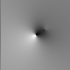
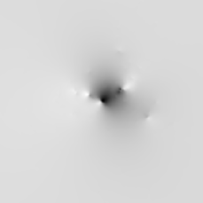
Figure 1: A comparison between our analytical description of the RS signal generated in a major merger (left panel) and the numerical simulation g24+200 described in the text and in Rasia et al. (2004) (right panel). The field of view is $2$ degrees on a side. The two clusters are placed at redshift $0.3$, have masses of $M_{1}=6\times 10^{14}M_{\odot}/h$ and $M_{2}=10^{15}M_{\odot}/h$ respectively, and they are falling onto each other with a relative velocity of $1800$ km/s. The analytical model represents the same merger of the numerical simulation, showing that our simple recipe provides a good description of the cluster merger. The total contribution of minor mergers is negligible, as explained in Section (4.2). The main difference is that the simulation includes the roughly spherical collapse of environmental DM onto the potential well. This collapse-induced signal has the shape of a negative peak with circular symmetry centered on the potential minimum. This contribution adds coherently to the signal of the two main halo mergers and is strictly related to the merging dynamic we want to estimate. Since we are ignoring this term, the resulting signal amplitude is smaller, making this choice conservative. In any case our filter can easily include this component, providing an estimate of the dynamic of the whole infalling dark matter and not only of the main merger components.

3 Distribution of physical parameters describing the merger

We investigate the probability distribution of the physical parameters describing a merger. We use the approach of Lacey & Cole (1993) based on the extended Press-Schechter formalism to model the distribution of cluster mergers in the Universe. This description basically relies on the probability of a region of mass $M_{1}$ having overdensity $\delta_{1}$ provided that, at the same point, the overdensity measured on a larger scale (corresponding to a mass $M_{2}$) is $\delta_{2}$. In other words, our starting point is the conditional probability of having $\delta_{1}$ on scales of $M_{1}$, given that on scales corresponding to $M_{2}$ the density contrast is $\delta_{2}$:

$$\begin{array}[]{ll}\displaystyle f(\delta_{1},M_{1}\big{|}\delta_{2},M_{2})dS_{1}=&\displaystyle\frac{\delta_{1}-\delta_{2}}{\sqrt{2\pi}(S_{1}-S_{2})^{3/2}}\times\\ &\displaystyle\exp{\biggl{[}-\frac{(\delta_{1}-\delta_{2})^{2}}{2(S_{1}-S_{2})}\biggr{]}}dS_{1}\,.\end{array}$$ (3)

Here, $S_{i}$ refers to the variance of the $\delta$ field on the scale of mass $M_{i}$, $S_{i}\equiv\langle\sigma(M_{i})^{2}\rangle$. Via the Bayes theorem, it is possible to compute the reverse probability, i.e., the probability of having a region of mass $M_{2}$ with overdensity $\delta_{2}$ given that on scale of $M_{1}$ the density contrast is $\delta_{1}$. If one introduces now the rate of growth of density fluctuations in linear theory, then this reverse probability can be understood as the rate at which a given halo collects matter:

$$\begin{array}[]{lll}\displaystyle{\cal R}(M_{1},\Delta M,z)\equiv&\frac{d^{2}p}{d\Delta Mdz}=&\displaystyle\sqrt{\frac{2}{\pi}}\frac{\delta_{sc}}{D(z)^{2}S_{2}}\times\\ &&\displaystyle\biggl{|}\frac{dD(z)}{dz}\biggr{|}\biggl{|}\frac{d\sigma(M_{2})}{dM_{2}}\biggr{|}\frac{1}{\left(1-\frac{S_{2}}{S_{1}}\right)^{3/2}}\times\\ &&\displaystyle\exp{\left[-\frac{\delta_{sc}^{2}}{2D(z)^{2}}\;\left(\frac{1}{S_{2}}-\frac{1}{S_{1}}\right)\right]}\,,\end{array}$$ (4)

where, $\delta_{sc}$ stands for the spherical collapse critical overdensity, and $\Delta M$ is the amount of mass being collected by the halo of mass $M_{1}$, so that $M_{2}=M_{1}+\Delta M$. The quantity $D(z)$ is the linear growth factor of density perturbations. When compared to numerical simulations, this formalism is able to reproduce approximately the halo merger history (e.g. van den Bosch, 2002). However, as noted by Benson et al. (2005), it has some intrinsic inconsistency due to its asymmetry in the arguments $M_{1}$ and $\Delta M$. In fact, the amount of clusters of mass $M_{1}$ to which clusters of mass $\Delta M$ are merging does not equal the number of clusters of mass $\Delta M$ to which clusters of mass $M_{1}$ are merging. We overcome this problem by defining the number of mergers of clusters of masses $M_{1}$ and $\Delta M$ as:

$$\begin{array}[]{ll}\displaystyle N_{merg}(M_{1},\Delta M,z)\equiv&\frac{1}{2}\biggl{[}{\cal R}(M_{1},\Delta M,z)\;n(M_{1},z)+\\ &\displaystyle{\cal R}(\Delta M,M_{1},z)n(\Delta M,z)\biggr{]}\Delta z\,,\\ \end{array}$$ (5)

where $n(M,z)$ represents the number density of haloes of mass $M$ at redshift $z$, (Press & Schechter, 1974). Since Equation (4) provides a merger rate, we must multiply it by the finite redshift interval $\Delta z$ which is taken to be equal to the dynamical time of the final cluster (approximated by $t_{dyn}(z)\simeq 0.09/H(z)$, with $H(z)$ the Hubble constant (Enßlin & Röttgering, 2002). Although this description of the halo merger rate might not be accurate, it should still provide a consistent description of the halo formation history.

We follow the model given in, Sarazin (2002), when assigning distances and velocities to the merging clusters. The typical initial distance between a pair of clusters, following Equation (10) in Sarazin (2002), may be approximated as

$$d_{0}\simeq 4.5\;\;\biggl{(}\frac{t(z)}{10^{10}\,yr}\biggr{)}^{2/3}\mbox{Mpc},$$ (6)

where $t(z)$ is the cosmic time. We assume that the probability of finding two merging clusters at a given distance $r\,(0<r<d_{0})$ is directly proportional to the time spent by those clusters in the interval $[r,r+dr]$, that is,

$$p(r)\propto\frac{1}{v(r)},$$ (7)

where $v(r)$ is the relative infall velocity of the clusters, given by

$$v(r)\simeq v_{0}\;\;\sqrt{\frac{M_{1}+\Delta M}{10^{15}\;M_{\odot}}}\sqrt{\frac{r}{d_{1}}\biggl{(}1-\frac{r}{d_{0}}\biggr{)}}.$$ (8)

In this equation, $v_{0}=2930$ km s^-1 and $d_{1}=$1 Mpc, and we ignore the angular momentum of the merging system. Putting all this together, we end up with a semi-analytical model of the merging cluster population in our universe, and of their velocities. Finally, we assume an isotropic distribution for the orientation of the merger plane with respect to the observer.

4 Observational strategy

The millimetric observations of upcoming experiments will provide extensive catalogues of galaxy clusters detected through their thermal SZ effect (tSZ), together with estimates of their masses and their geometrical properties. The tSZ effect can be measured separately from the other effects due to its unique spectral dependence. The data of CMB temperature fluctuations will contain signatures of the RS effect we aim to detect, together with the following components which will be regarded here as contaminants: the primordial CMB field, the instrumental noise, the lensing of the CMB anisotropies induced by the matter present along the line of sight, and the kinematic SZ (kSZ) effect generated by the cluster peculiar velocity with respect to the Hubble flow. As long as the contaminants show different spatial characteristics compared to the signal we are trying to unveil (the RS effect), it is possible to define a filter which optimally reduces the impact of those sources of noise. Regarding this, instrumental noise will be assumed to be scale–free white noise, i.e., to have the same power at all scales. The intrinsic CMB fluctuations usually have (if clusters are not too close) scales larger than those of the RS signal. On the other hand, the kSZ and the tSZ residuals are confined to the region of the cluster where the gas is located. Compared to these scales, the RS is usually broader.

However, if a contaminant shows spatial power on scales which are too close to those of the signal, only a more direct approach can be performed. This turns out to be the case for the anisotropies introduced by the lensing of the intrinsic CMB fluctuations. This component will require a separate processing (Section 4.1): from a template of the lensing-induced deflection field, we shall “deflect back” the data, in an attempt to subtract the effect of gravitational lensing on the CMB. This will allow us to minimize the impact of this contaminant.

Once the cluster lensing signal is reduced by this “de-lensing procedure”, an optimized filter will be applied to suppress the other noise terms and to estimate the RS effect amplitude. This amplitude depends on the cluster infall velocity, which is essentially the physical parameter we are measuring (see Equation 2). This filter incorporates in its definition two templates: one for the RS effect described in Section (2), parameterized by the mass which we assumed to be estimated from observations of the tSZ effect, and one for the kSZ effect. The second one could be directly derived from the millimetric observations by observing at $217\mbox{GHz}$ and filtering away the CMB features through a high–pass filter.

As we shall see, the resulting signal-to-noise ratio of a single merger is too small to provide a detectable signal. Thus it is necessary to average multiple measurements of many mergers. The detection of the cluster through their tSZ effect is already well described in other papers (e.g. Schaefer et al., 2004) so it will not be discussed here. We will now describe in detail the steps of the observational strategy summarized above.

4.1 De-lensing procedure

The CMB anisotropy produced by the gravitational lensing effect of galaxy clusters has a typical amplitude ten times larger than the RS anisotropy induced by the same clusters. These two effects arise from the same gravitational potential, so that their typical spectral scales are comparable and correlated in position and, although their patterns are not identical, the similarity of their power spectra complicates the use of any Wiener filter.

Therefore it is necessary to reduce the lensing effect before the application of any optimized filter. To achieve this, we propose to remap the observed data by applying a distortion which compensates, as accurately as possible, the cluster lensing effect.

To do this it is necessary to invert the lens equation $T(\@vec{\theta})=\tilde{T}(\@vec{\theta}-\@vec{\alpha}(\@vec{\theta}))$ by introducing the new coordinate $\@vec{\theta}^{\prime}=\@vec{\theta}-\@vec{\alpha}(\@vec{\theta})$. In this way it is possible to derive from the observed data $T$ the de-lensed map $\tilde{T}$ thanks to the deflection field template $\@vec{\alpha}$, according to

$$\tilde{T}(\@vec{\theta})=T(\@vec{\theta}+\@vec{\alpha}(\@vec{\theta}^{\prime}))\,.$$ (9)

Note that the deflection field has to be computed via an iterative procedure, because it is evaluated at the new coordinate $\@vec{\theta}^{\prime}$.

In order to build a deflection field template, we define the merger using two NFW haloes according to Equation (2). We assume that their masses are derived by the tSZ measurements, and for this reason we will consider some uncertainty in the mass determination. The assumption of spherical haloes is justified since the deflection field is roughly symmetric on large scales. Furthemore, the final estimate of the signal will be produced after stacking all available merger events.

Of course this procedure will – apart from the CMB – also distort the RS signal, the kSZ signal and the distribution of the instrumental noise. Because of this, the RS effect and the kSZ templates used in the optimal filter definition have to be corrected through the same process. This procedure leaves some randomly distributed residuals in the field, and some non-Gaussian features in the instrumental noise which will be ignored in the following analysis.

4.2 Filter

Once the cluster lensing contribution is minimized, the remaining data contaminants in the maps are the CMB primary anisotropy, the kSZ effect and the instrumental noise.

The Gaussian contribution of CMB and instrumental noise are fully described by their corresponding power spectra and can be filtered out by optimized filters. In particular, the CMB power spectrum shows an exponential cutoff around the arcminute scale due to Silk damping of primordial fluctuations. This angular scale is close to the typical one for distant galaxy clusters, and hence the CMB intrinsic fluctuations should make small contributions at the spatial frequencies we are interested in. For CMB experiments with very high–sensitivity on small–scale, such as ACT, SPT or the Atacama Large Millimeter Array we shall assume that the noise is spatially white, i.e., that it introduces the same amount of power in all scale.

Table 1: Main characteristics of the upcoming millimetric observatories ACT, SPT and of our simulated instrument. The second column gives the available frequency channels, the third column the angular resolution and the last column the relative sensitivity. We are reporting nominal sensitivities for ACT, and those of SPT correspond to one hour of observation.

	bands	FWHM	$\Delta$T/beam
	(GHz)	(’)	($\mu K$)
ACT	145, 225, 265	1.7, 1.1, 0.93	2, 3.3, 4.7
SPT	150, 219, 274	1, 0.69, 0.56	2.5, 3.0, 2.65
simulation	217	1	1

Figure 2: To give an intuitive view of how our filter works, we present here two simple examples where the signal and a contaminant of known spatial pattern have both Gaussian profiles with the same width. In the upper panel both signal and noise are positive and the sum of these contributions, the data, is given by the solid line, while the dashed line displays the resulting filter. In the bottom panel we only changed the sign of the amplitude of the noise, which now is negative. The estimator defined in Equation (15) is the integral of the solid line times the dashed one. In the first (upper panel) case, the filter is negative where the contaminant is positive, so that their product is negative and the contaminant contribution is subtracted. In the second case (bottom panel), both filter and contaminant are negative so that their product is positive and the negative contribution of the noise is compensated. This actually shows that the same filter provides an unbiased estimator also if only the variance of the contaminant amplitude is known. That is, the sign of the contaminant is irrelevant to the filter, and this reflects the statistical nature of our filter.

We present here an optimally matched filter (derived detail in Appendix A), which maximizes the signal-to-noise ratio by processing the signal in the Fourier domain. A similar filter construction was proposed by Haehnelt & Tegmark (1996) in order to extract the kSZ signal from single clusters. However, that method considered the CMB and instrumental noise the only sources of confusion when trying to recover the kSZ signal. Our filter is defined in a slightly more general context. It provides an estimate of the amplitude of a signal with a known spatial template and is to be measured despite a presence of homogeneous noise with a known spatial power spectrum and an arbitrary number of other contaminants following known spatial patterns. Hence, the total observed data can be modeled by

$$s(\@vec{r})=A\tau(\@vec{r})+n(\@vec{r})+\sum_{i=1}^{M}v_{i}z_{i}(\@vec{r})\,,$$ (10)

where $A$ is the amplitude of the signal, $\tau(\@vec{r})$ is the signal shape, $n(\@vec{r})$ is a Gaussian random noise with a known power spectrum $P_{n}(k)$, and $z_{i}(\@vec{r})$ are $M$ noise sources with an amplitude $v_{i}$. Note that this model can a priori be applied to different problems. For instance, in weak lensing observations, where it is necessary to take into account the noise introduced by stars, bright galaxies and the cluster core itself, this filter allows improved results obtained with standard matched filters (e.g. Maturi et al., 2005b).

The Gaussian noise contribution $n(\@vec{r})$ will contain the CMB temperature fluctuations, the instrumental noise, and all the noise sources which can be modeled as Gaussian random fields. In this case, the filter derived in Appendix (A) takes the form

$$\Psi(\@vec{k})=\frac{\lambda T(\@vec{k})-B_{1}Z_{1}(\@vec{k})-B_{2}Z_{2}(\@vec{k})}{P_{n}(k)}\,,$$ (11)

where $P_{n}(k)=P_{CMB}(k)+P_{inst.}(k)$ is the total Gaussian noise power spectrum, including the CMB and the instrumental noise. In our case, we introduce two spatially characterised contaminants ($M=2$), that is, the kSZ signal of the two merging haloes $Z_{1}(\@vec{k})$ and $Z_{2}(\@vec{k})$. The normalization of the first term in the numerator can be expressed as $\lambda=(1+D)/C$, with

$$C=\left\{|T|^{2}/P_{n}\right\}$$ (12)

and

$$D=\Re\left(\left\{\frac{T^{*}\left(B_{1}Z_{1}+B_{2}Z_{2}\right)}{P_{n}}\right\}\right)\,.$$ (13)

The coefficients $B_{i}$ are given by

$$B_{i}=\sigma_{vi}^{2}\{Z_{i}^{*}\Psi\}\,,$$ (14)

and the estimate of the RS effect amplitude $\bar{A}$ will be provided by

$$\bar{A}=\left\{S\Psi^{*}\right\}\,.$$ (15)

In these equations, the bracket notation $\{\,f\,\}$ stands for a double integral in the k–space of a general function $f(\@vec{k})$ as defined in Equation (20). The quantity $\sigma_{vi}^{2}$ represents the variance of the ith contaminant amplitude, and the symbol $\Re$ denotes “real part”.

It is clear from Equation (11) that the filter can be split into two components. The first, ($T^{*}/P_{n}$), maximizes the sensitivity at the spatial frequencies where the signal $T$ is large and the noise power spectrum $P_{n}$ is small, as opposed to the second ($-(B_{1}Z_{1}+B_{2}Z_{2})/P_{n}$), which underweights the regions where the $Z_{i}$ components are important and correlated with the filter itself. Note that since the filter $\Psi$ is present in the definition of the $B_{i}$ coefficients, the final form of the filter must be computed iteratively.

Figure 3: Spatial distribution of the signals considered in a major merger at $z=0.3$, of two haloes with masses $10^{15}M_{\odot}$ and $5\times 10^{14}M_{\odot}$, and with an infall velocity of $1500km/s$ at $45$ degrees with respect to the line of sight. Since the two haloes are colliding, the RS effect (top left) of both components adds constructively, amplifying the resulting signal in the region between them. The kSZ effect (top right) shows a typical dipolar pattern reflecting opposite velocities along the line of sight. The anisotropy introduced by the lensing effect has a complex shape, since it depends on the configuration of both haloes and the CMB gradient (bottom left). The bottom right panel shows our filter. It is high–pass in order to suppress the CMB primary anisotropy noise contribution. The temperature amplitudes of these panels along the line containing the haloes are displayed in Figure (4).

Figure 4: Comparison between the filter profile and the different components under consideration. The top left panel shows the de-lensed RS effect superimposed on the filter. Note the sudden change of amplitude and sign of the filter close to the cluster cores. The top right panel displays the kSZ effect and the filter, whereas the bottom left one shows how the de–lensing procedure acts on the kSZ effect, shrinking its profile and shifting the peaks closer to the center. In the bottom left panel we show how the de–lensing procedure acts on the kSZ effect, by shrinking its profile and shifting the peaks closer to the center. The bottom right panel compares our filter (new filter) with the filter originally proposed by Seljak & Zaldarriaga (2000) (H & T 1996). The difference between these two filters is negligible when the contaminant given by kSZ effect (the $Z$ template) is orthogonal to the signal, otherwise it becomes relevant.

The template for the RS effect ($\tau(\@vec{r})$) was modeled by two merging NFW haloes, as explained in Section (2). The contribution from small merging substructures should be negligible, since our filter is a weighted integral over the whole field (Equation 15), and these minor mergers are odd functions of typical scales much smaller than the one of the filter.

The kSZ masks are applied as a weight templates and are not directly subtracted from the input data. This makes the accuracy to which the templates are known uncritical. For this reason it is possible to use the observations at 217 GHz (the frequency at which the tSZ vanishes to a good approximation) as a good template for the kSZ. There might be some tSZ residuals, together with the lensing and RS signals, but their contribution is negligible for the filter construction. Again, this is because the filter does not subtract this template directly from the maps, which of course would erase all the RS signal we are searching for, but it only weights down optimally the regions contaminated by the kSZ effect.

5 Simulation of the observations

To test the described procedure we performed simulations of the secondary anisotropies induced on the CMB by binary cluster mergers in a cosmological context. For the two merging haloes, we adopt a NFW profile for the dark matter component and a spherical isothermal sphere (SIS) for the gas distribution. We ignore tidal effects and the hydrodynamic processes involved in the interaction between the intra-cluster gas (ICM) of the two haloes. For our purpose, the model adopted gives a sufficiently realistic representation of RS, kSZ, lensing effect and instrumental noise.

We adopt a standard $\Lambda$CDM cosmology with a density contribution from dark matter, baryons and cosmological constant of $\Omega_{\mathrm{DM}}=0.27$, $\Omega_{\mathrm{B}}=0.044$, and $\Omega_{\Lambda}=0.7$, respectively. The Hubble constant was set to $H_{0}=100\,h\,\mathrm{km\,s^{-1}\,Mpc^{-1}}$ with $h=0.7$ (Bennett et al., 2003).

We simulated the CMB primary anisotropies as Gaussian random fields with a resolution of $1024^{2}$ pixels and a field of view of $120^{\prime}$. The CMB power spectrum used was computed using CMBEASY (Doran, 2003), assuming a re–ionization fraction of $0.1$ at redshift $z=6.2$ and a present helium abundance of $0.24$. The field size ensures an adequate sampling of the CMB multipoles, and permits the retention of only the central quarter of the whole field, avoiding the boundary effects of the Fourier transforms.

For an isothermal cluster with negligible internal motions the kSZ and the tSZ effects are proportional to one another:

$$\frac{\delta T_{tSZ}}{T_{0}}(\theta)=g_{tSZ}(\nu)\;\frac{k_{B}T_{e}}{m_{e}c^{2}}\;\int\;dl\;n_{e}\sigma_{T},$$

$$\frac{\delta T_{kSZ}}{T_{0}}(\theta)=\frac{{-\bf v}\cdot{\bf n}}{c}\;\int\;dl\;n_{e}\sigma_{T}.$$ (16)

in the previous equation $g_{tSZ}(\nu)$ provides the (non–relativistic) frequency dependence of the tSZ effect in temperature, and $m_{e}$, $n_{e}$ and $T_{e}$ are the electron mass, number density and temperature, respectively. The integrals are performed along the line of sight given by the pointing direction ${\bf n}$, and the angle $\theta$ separates the line of sight from the cluster center. The dependence of the integral on the line of sight translates into the angular dependence. In particular, we assumed the ICM of each merger component to be distributed as an isothermal sphere with a radial $\beta$–profile with $\beta=1$ (i.e. a King profile). We based our strategy on observations at $217\leavevmode\nobreak\ GHz$, where the tSZ effect vanishes. Thus the SZ contamination is given only by the kSZ component.

The lensing effect on the CMB is described by the lens equation:

$$T(\@vec{\theta})=\tilde{T}[\@vec{\theta}-\@vec{\alpha}(\@vec{\theta})]\approx\tilde{T}(\@vec{\theta})-\@vec{\nabla}\tilde{T}(\@vec{\theta})\cdot\@vec{\alpha}(\@vec{\theta})\,,$$ (17)

where $T$ is the observed temperature map, $\tilde{T}$ is the un-lensed CMB and $\@vec{\alpha}$ is the cluster deflection angle. Bartelmann (1996) wrote an analytic expression for the deflection angle caused by a NFW halo, and, by using it we can compute the $\@vec{\nabla}\tilde{T}\cdot\@vec{\alpha}$ term, which represents the secondary anisotropy given by the lensing effect (Seljak & Zaldarriaga, 2000). The linear expansion is justified as long as the variations of the local CMB temperature gradient are small on a deflection angle scale.

The RS and kSZ effects were computed after introducing this deflection angle into Equation (2). The distribution of cluster mergers in the universe is described according to the equations presented in Section (3). The number of clusters $N_{M,z}$ was computed with that formalism on a finite number of mass-redshift cells. Then, for each cell, we randomly distributed $N_{M,z}$ clusters with redshifts and masses enclosed in the cell range.

We included in our simulation the noise from a single dish telescope with a resolution of $1$ arcminute and a sensitivity of $1\mu K$ per beam. This noise was modeled as a Gaussian field with the following power spectrum

$$C_{l}^{\mathrm{noise}}=w^{-1}\exp\left[\frac{l(l+1)\,\mathrm{FWHM}^{2}}{8\ln 2}\right]\;,$$ (18)

where $\Delta T/T$ is the sensitivity of the experiment in on the scale of the beam and $w^{-1}:=(\Delta T/T\,\mathrm{FWHM})^{2}$ (Knox, 1995). The exponential expresses the increasing weight of noise when probing sub-beam scales. These characteristics of the simulated instrument are compatible with the next–generation millimetric observatories, as shown in Table (1). We have not included the parameters corresponding to ALMA because our filter should have then included the synthesized beam of the interferometer, but its sensitivity should enable it to detect signals of amplitudes similar and smaller than those of the RS effect considered here.

6 Results

In order to probe the ability of our extended filter in separating the RS signal, we have prepared three different mock catalogues of cluster mergers following the recipe described in Section (4). These catalogues were generated using three minimum mass thresholds of $5\times 10^{13}M_{\odot}$, $8\times 10^{13}M_{\odot}$ and $10^{14}M_{\odot}$, and contain $6807$, $266$ and $28$ cluster mergers, respectively.

The analysis of the mock catalogues was carried out in two ways, corresponding to the degree of knowledge of the template maps.

• Case A. We assume that we know the masses of the merging clusters with an uncertainty of $30\%$. These values are used to build the kSZ and the RS templates. For the halo radial velocity, we use Equation (14) with an expected velocity dispersion $\sigma_{v}\approx 300km/s$.

• Case B. Similar to the previous case but, instead of building a kSZ template, we shall use directly the millimetric observations of the kSZ effect, which account for the kSZ asymmetries caused by internal motions (Nagai et al., 2003). The presence of the RS effect in these maps is negligible and does not affect the filter definition. The only problem related to this procedure is the noise present in the kSZ maps which is included in the filter construction. A low pass filter of the map should reduce the problem. In our simulation we directly used the kSZ plus the RS maps, assuming that a noise suppression procedure had already been applied to those maps.

The results for Case A are presented in Table (2). The columns represent: first, the lower limit adopted to build the cluster samples; second, the number of objects in the sample; third, the average RS signal of the sample; and last, the estimate.

Even with a moderate size cluster merger catalogue ($266$ clusters), the significance of our method approaches the 2-$\sigma$ level in the detection of the RS signal. Since we are observing different mergers, and the errors in different mergers are uncorrelated, our Poissonian error bars scale is the inverse square root of the number of mergers.

Table 2: RS amplitude estimates for three mass selected cluster subsamples, defining the filter with a $30\%$ mass uncertainty and using only the expected velocity dispersion $\sigma_{v}\approx 300\leavevmode\nobreak\ km/s$. Error bars in the last two columns correspond to the combined measurement from all clusters in the corresponding sample and with the coresponding filters (case A and B).

mass	clusters	simulation	estimate A	estimate B
$M_{\odot}$		$\mu K$	$\mu K$	$\mu K$
$M>5\times 10^{13}$	6807	0.18	0.13 $\pm$ 0.03	0.16 $\pm$ 0.03
$M>8\times 10^{13}$	266	0.25	0.24 $\pm$ 0.14	0.13 $\pm$ 0.19
$M>1\times 10^{14}$	28	0.28	0.29 $\pm$ 0.42	0.05 $\pm$ 0.68

The results for Case B are also presented in Table (2). As one can see, RS signal detection is still possible. Comparing these results with those of the previous table, it is clear that the filter efficiency is not significantly affected. This is mainly due to the statistical nature of our filter: it relies not on the accuracy of our templates for each merger, but on the accuracy of our templates when describing the average spatial properties of the kSZ and RS signals. Indeed, in principle one could also use the same average RS and kSZ templates for all mergers. The precision of our method is hence limited by the number of available mergers according to Poisson statistics.

We recall that these results have been obtained ignoring the component of the RS signal of galaxy clusters given by the collapse of the environmental dark-matter in the potential well of the system. The inclusion of this component would increase the signal-to-noise ratio of the estimates.

7 Conclusions

We presented a method to extract the kinematic properties of major merger events of galaxy clusters by means of their RS signal, which is observable at centimeter/millimeter wavelengths. The RS effect is a secondary anisotropy of the CMB produced by the time variation of the gravitational potential along the line of sight. In this particular case, the main contribution comes from the infall motion of the merging components, so that the total signal is a measurement of the convergence of the projected perpendicular momentum of the system (see Paper I).

We proposed a method to extract this RS signal from a sample of cluster mergers observed at millimetric wavelengths. These observations will be contaminated by the primordial CMB fluctuations, the kinematic SZ signal and the lensing effect from the clusters, together with the instrumental noise. We assumed that the thermal component of the SZ effect can be subtracted by multi-frequency observations, given that we know its frequency dependence.

The RS effect amplitude in one single merger event is much smaller than all the other components and thus only a statistical detection of the signal may be achieved. To maximize the signal-to-noise ratio and decrease the number of mergers that we need to co-add, we can apply a filter which enhances the RS signal above the other components. Therefore, we proposed in Section (4.2) an extended version of a matched filter presented by Haehnelt & Tegmark (1996). A complete derivation of our filter is given in Appendix (A). It requires as input the power spectra of the CMB and the instrumental noise, plus two templates, one for the RS signal and another for the contaminating kSZ effect. These templates can be simple analytic models parameterized with the mass estimates provided by the tSZ measurements, and with the expected average velocities. We would like to note that the filter construction is general so that it can be applied to other problems like the extraction of gravitational lensing on CMB maps (e.g. Haehnelt & Tegmark, 1996; Maturi et al., 2005a) or on background galaxies (Maturi et al., 2005b).

We showed that the developed filter can control the contamination from all signals except CMB lensing. This is because the RS and the lensing effect originate from the same gravitational deflection field, and thus their spatial frequencies are similar. Therefore, we included in our pipeline an additional step before the filter application, i.e. a “de–lensing” procedure. We propose remapping the input data according to the inverse template deflection field, again parameterized by the tSZ mass estimate.

The method was applied to mock catalogues of cluster mergers. Our results show that the RS signal of merging clusters could be measured with this method after observing of the order of $1,000$ cluster mergers. These numbers will be achieved by combining the expected yields of the upcoming high–resolution millimetric surveys (e.g. ACT, SPT, ALMA). Assuming a fraction of 30% for the number of mergers over the number of clusters, a RS detection will be feasible if future SZ surveys are able to perform sensitive observations of the order of $10^{4}$ clusters.

Appendix A Optimal filter

We aim to build an optimized filter $\psi(\@vec{r})$ to extract from a noisy data set $s(\@vec{r})$ the best estimate of amplitude $A$ of any signal with a known spatial shape $\tau(\@vec{r})$:

$$s(\@vec{r})=A\tau(\@vec{r})+n(\@vec{r})+z(\@vec{r})\,.$$ (19)

We assume $n(\@vec{r})$ to be a Gaussian random noise with zero mean ($\langle n(\@vec{r})\rangle=0$) and known power spectrum $P_{N}(\@vec{k})$; and $z(\@vec{r})=\sum_{i=1}^{M}v_{i}z_{i}(\@vec{r})$ to be the sum of $M$ different noise components with unknown amplitude $v_{i}$ with zero mean ($\langle v_{i}\rangle=0$) but known variance $\sigma_{v\,i}$.

We define the integral of a general function $f(\@vec{k})$ as

$$\{f\}\equiv\int\frac{d^{2}k}{(2\pi)^{2}}f(\@vec{k})\,.$$ (20)

Since the Equation (19) is linear in $A$, its most general linear estimate in the Fourier domain can be written as

$$\bar{A}=\left\{S\Psi^{*}\right\},$$ (21)

where the capital letters refer to Fourier transforms. This estimate is required to have a bias $b=\langle\bar{A}-A\rangle=0$. It has a variance $\sigma^{2}=\langle(\bar{A}-A)^{2}\rangle$ given by

$$b=A\left(\left\{T\Psi^{*}\right\}-1\right)\,,$$ (22)

$$\sigma^{2}=b^{2}+\left\{|\Psi|^{2}P_{n}\right\}+\left\{\@vec{Z}^{t}\Psi^{*}\right\}\@vec{V}\left\{\@vec{Z}^{*}\Psi\right\}\,,$$ (23)

where we grouped the collection of the $M$ noise contributions $Z_{i}(\@vec{k})$ in a vector $\@vec{Z}(\@vec{k})$ and defined the covariance matrix $\@vec{V}$ of its components as $V_{ij}=\langle v_{i}v_{j}\rangle$.

Since we are interested deriving a filter which minimizes the estimate variance maintaining the unbias condition $b=0$, we introduce the Lagrangian multiplier $\lambda$ and search for the filter function $\Psi$ which minimizes the action $L=\sigma^{2}+\lambda b$, obtaining

$$\Psi(\@vec{k})=\frac{\lambda T(\@vec{k})-\@vec{Z}^{t}(\@vec{k})\@vec{V}\left\{\@vec{Z}^{*}\Psi\right\}}{P_{N}(k)}\,,$$ (24)

where the apex $t$ is for the transposed vectors.

The normalization factor $\lambda$ is obtained by substituting Equation (24) in Equation (22), yielding

$$\lambda=\frac{1+\Re\left(\left\{T^{*}\@vec{Z}^{t}/P_{n}\right\}\@vec{V}\left\{\@vec{Z}^{*}\Psi\right\}\right)}{\left\{|T|^{2}/P_{n}\right\}}\,,$$ (25)

where $\Re$ is for the real part.

As is clear from Equation (24), the filter has to be computed through an iterative procedure, where the starting point can be the filter with the variance matrix $\@vec{V}$ equal to the null matrix (this is essentially the filter originally proposed by Haehnelt & Tegmark (1996)). This iterative procedure is required since the filter evaluation requires the correlation between the filter itself and the noise sources.

The simple intuitive interpretation of this filter is that the first term $T/P_{n}$ maximizes the sensitivity on the spatial frequencies where the signal $T$ is large and the noise power spectrum $P_{n}$ is small. At the same time the second term $(\@vec{Z}^{t}\@vec{V}\{\@vec{Z}^{*}\Psi\})/P_{n}$ introduces a weighted mask which takes into account the correlation between the filter $\Psi$ and all the $Z_{i}$ noise components, as well as the correlation between the different $Z_{i}$ noise components. It is important to note that the filter $\Psi$ does not apply a mask only by subtracting the $Z_{i}$ templates from the input data, leading to spurious residuals, but it down-weights the influence of the regions where the $Z_{i}$ components are dominant and correlated with the filter itself. This means it is not critical to have a very accurate template for the noise sources, in order to apply the filter properly. It is sufficient to have a simple model which represents their average shapes.

The derived filter satisfies a generalized problem, where the noise sources $v_{i}Z_{i}$ can also be correlated, but in the majority of cases the noise sources will be uncorrelated, either due to them having different positions or their amplitudes $\@vec{v}$ being mutually uncorrelated. In this case the matrix $\@vec{V}$ is diagonal and the filter function simplifies to

$$\Psi(\@vec{k})=\frac{\lambda T(\@vec{k})-\sum_{i}^{M}B_{i}Z_{i}(\@vec{k})}{P_{n}(k)}\,,$$ (26)

where the normalization can be written as $\lambda=(1+D)/C$, the denominator $C$ is given by

$$C=\left\{|T|^{2}/P_{n}\right\}$$ (27)

and the $B_{i}$’s and D are defined as

$$B_{i}=\sigma_{vi}^{2}\{Z_{i}^{*}\Psi\}\,,$$ (28)

and

$$D=\Re\left(\left\{\frac{T^{*}\sum_{i}^{M}B_{i}Z_{i}}{P_{n}}\right\}\right)\,.$$ (29)

With this assumption, valid for many applications, the filter acquires this simple expression.