Depolarization canals and interstellar turbulence

Abstract

Recent radio polarization observations have revealed a plethora of unexpected features in the polarized Galactic radio background that arise from propagation effects in the random (turbulent) interstellar medium. The canals are especially striking among them, a random network of very dark, narrow regions clearly visible in many directions against a bright polarized Galactic synchrotron background. There are no obvious physical structures in the ISM that may have caused the canals, and so they have been called Faraday ghosts. They evidently carry information about interstellar turbulence but only now is it becoming clear how this information can be extracted. Two theories for the origin of the canals have been proposed; both attribute the canals to Faraday rotation, but one invokes strong gradients in Faraday rotation in the sky plane (specifically, in a foreground Faraday screen) and the other only relies on line-of-sight effects (differential Faraday rotation). In this review we discuss the physical nature of the canals and how they can be used to explore statistical properties of interstellar turbulence. This opens studies of magnetized interstellar turbulence to new methods of analysis, such as contour statistics and related techniques of computational geometry and topology. In particular, we can hope to measure such elusive quantities as the Taylor microscale and the effective magnetic Reynolds number of interstellar MHD turbulence.

1 The promise and pitfalls of radio polarization

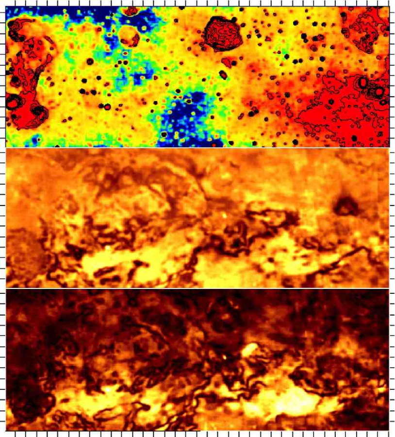
Figure 1: A $24^{\circ}\times 9^{\circ}$ section of the $1.4\,\mathrm{GHz}$ Effelsberg Medium Latitude Survey centred at $(l,b)=(162^{\circ},0^{\circ})$ (Reich et al. [2004]). Top: total intensity, with large-scale structure added from Dwingeloo data. Middle: polarized intensity, also including the Dwingeloo large-scale structure. Bottom: polarized intensity observed with the Effelsberg telescope with large scale structure missing. Note the strong difference between the (preliminary) absolutely calibrated polarized intensity map (middle) and the map with artificial base-levels (bottom).

High-resolution maps of the Milky Way synchrotron emission show a complex, irregular system of polarized and depolarized structures (Wieringa et al. [1993], Uyanıker et al. [1998b], Duncan et al. [1999], Gray et al. [1999], Haverkorn et al. [2000], Gaensler et al. [2001], Wolleben et al. [2006]). Many polarized structures can be attributed to objects in the interstellar medium (ISM), such as supernova remnants and shock fronts. These objects are usually bright in total intensity as well. However extended, diffuse polarized emission is also rich in structure which most plausibly arises from propagation effects as the radiation passes through the random ISM. As illustrated in Fig. 1, much of this structure is not mirrored in the total synchrotron intensity so the structure in polarization is not primarily caused by variations in emissivity. At low frequencies, the cloudy appearance of polarized intensity maps differs between adjacent, narrow frequency bands (Haverkorn et al. [2003]) strongly suggesting that the polarization varies with wavelength and so a connection with Faraday rotation is plausible. Random fluctuations in the magnetized ISM — caused by its turbulent flows, for example — leave their fingerprint in the random appearance of polarized intensity maps. If a connection can be established between measurable properties of the radio maps to the physics of the ISM, a powerful new source of information about the dynamic state of the interstellar plasma will become available, particularly its little studied magnetic properties. Similarly, a reliable separation of the Milky Way synchrotron polarized foreground from cosmological signals, either through the creation of templates from low-frequency data or through statistical analysis, requires a thorough understanding of the origins of structure in the diffuse polarized emission. In the context of cosmological studies, the effects of the ISM on the polarized emission propagating through it are especially important.

One of the most striking features of the maps is the twisting network of narrow, dark canals running through regions of bright polarized intensity, clearly visible in Fig. 1 at $1.4\,\mathrm{GHz}$ and common in other maps at this frequency (Uyanıker et al. [1998b], Gaensler et al. [2001]) and longer wavelengths (Haverkorn et al. [2000]). The observed canals have the following properties:

1. the observed polarized intensity falls to zero, because the polarization angle changes by $90^{\circ}$ across the canal;

2. a canal is one telescope beam wide;

3. a canal passes through a region of significant polarized intensity;

4. the canal is not related to any obvious structure in the total intensity.

Care in interpreting the observations is especially important in the case of polarized emission: interferometer observations miss emission at large scales (determined by their shortest baseline), and single-dish surveys often have arbitrarily set base-levels around their edges. Correcting for the missing large-scale structure involves adding a smoothly varying signal to the Stokes parameters. In the case of total intensity (Stokes $I$) the consequences are easily predictable. However, the Stokes parameters $Q$ and $U$ are not positive definite and therefore algebraic addition of a smooth component can create and/or remove zeros in either. Hence minima in polarized intensity $(Q^{2}+U^{2})^{1/2}$ can become maxima and vice versa. The effect of absolute calibration on the polarization angle $\Psi=\frac{1}{2}\arctan{(U/Q)}$ can be equally counter-intuitive. Reich et al. ([2004]) clearly identify and discuss these problems. The dramatic effect the missing data can have on the appearance of the polarization pattern can be seen by comparing the bottom two panels of Fig. 1. It is clear that unless statistical parameters can be identified that are independent of the $Q$ and $U$ intensity values, polarization surveys should be tied to an absolutely calibrated reference frame (Uyanıker et al. [1998a], Reich et al. [2004]). The recent absolutely calibrated all-sky survey at $1.4\,\mathrm{GHz}$ by Wolleben et al. ([2006]) will be a mine of useful information for polarization studies. Haverkorn et al. ([2004]) argue that if fluctuations in Faraday rotation measure are sufficiently strong and of a small scale, the resulting structure in $Q$ and $U$ can be of such a small scale that the missing short spacings will not cause a problem. In other words, $Q$ and $U$ may have no large scale structure; this can easily happen at metre wavelengths.

Two theories accounting for the origin of the canals have been proposed: one invokes strong plane-of-sky gradients or discontinuities in Faraday rotation measure in a foreground screen between the emitting region and the observer (Haverkorn et al. [2000, 2004]; Haverkorn & Heitsch [2004]) and the other proposes differential Faraday rotation along the line-of-sight through the emitting layer (Beck [1999], Shukurov & Berkhuijsen [2003]).

In this review we summarize recent work on the interpretation of depolarized canals and provide a more detailed explanation of some analytic results than is available in the readily accessible literature. After introducing basic equations and defining our notation in Section 2, we describe the effects of differential Faraday rotation and Faraday screens, demonstrate how canals are formed by the two proposed mechanisms and discuss how observable quantities behave in the vicinity of a canal in each case. Then in Section 3 we turn to the interpretation of the properties of the canals in terms of the physical state of the ISM. In Section 3.1 the case of differential Faraday rotation is discussed in the context of the statistical properties of contours of a random field and we show how canals of this type can yield information about the smallest scales of ISM turbulence. Similar techniques can be applied to canals produced by Faraday screens, and more generally to contours of any randomly distributed observable quantity. Section 2.2 demonstrates that true discontinuities in Faraday rotation are required if a foreground screen is to produce canals similar to those observed. In the case that these discontinuities are shock fronts originating from supernovae, we show in Section 3.2 how the distance between canals is related to the separation of shock fronts.

2 The complex polarization, Stokes parameters and depolarization

The complex polarization is commonly written as

$$\mathcal{P}=p_{0}\frac{\int_{V}W(\mathbf{r})\epsilon(\mathbf{r})\exp{[2i\psi(\mathbf{r})]\,\mathrm{d}V}}{\int_{V}W(\mathbf{r})\epsilon(\mathbf{r})\ \mathrm{d}V},$$ (1)

where $p_{0}\simeq 0.7$ is the maximum degree of polarization for synchrotron emission (a function of the spectral index), $W$ is the beam profile around a given position in the sky, $\epsilon$ is the synchrotron emissivity, and $\psi$ is the local polarization angle. The integrals are taken over the volume of the beam cylinder and $\mathbf{r}=(x,y,z)$ specifies a location with respect to the sky plane ($x,y$) and the line of sight, $z$. The modulus and argument of $\mathcal{P}$ are the observed degree of polarization $p$ and polarization angle $\Psi$ respectively,

$$\mathcal{P}=p\,\exp{(2i\Psi)}.$$ (2)

When polarized radio emission propagates through magnetized and ionized ISM, the local polarization angle $\psi$ undergoes Faraday rotation:

$$\psi(\mathbf{r})=\psi_{0}(\mathbf{r})+\phi(\mathbf{r})\;,$$ (3)

where $\psi_{0}$ is the intrinsic polarization angle (perpendicular to the magnetic field component transverse to the line of sight at the point of emission),

$$\phi=K\lambda^{2}\int^{\infty}_{z}n_{\mathrm{e}}(z^{\prime})B_{z}(z^{\prime})\,\mathrm{d}z^{\prime},$$ (4)

$K=0.81\,\mathrm{rad}\,\mathrm{m}^{-2}\,\mathrm{pc}^{-1}\,\mathrm{cm}^{3}\,\mu\mathrm{G}^{-1}$ is a constant, $n_{\mathrm{e}}$ is the density of free thermal electrons, $B_{z}$ is the component of the magnetic field along the line of sight $z$, $\lambda$ is the wavelength and the observer sits at $z=\infty$. The Faraday depth, at a position $(x,y)$ in the plane of the sky, is defined as,

$$F(x,y)=\phi(-\infty)=K\lambda^{2}\int^{\infty}_{-\infty}n_{\mathrm{e}}(z)B_{z}(z)\,\mathrm{d}z\;.$$

and $\phi(z)$ is known as the Faraday depth to a position $z$ (cf. Eilek [1989]). $F$ and $\phi(z)$ are convenient variables to work with; $\phi(z)$ gives the change in polarization angle of a photon of wavelength $\lambda$ passing through the region $z<z^{\prime}<\infty$, and $F$ is the maximum amount of Faraday rotation in a given direction in the sky. Note that $F/\lambda^{2}$ can differ strongly from the observed Faraday rotation measure $\mathrm{RM}=\mathrm{d}\psi/\mathrm{d}\lambda^{2}$. For example, $\mathrm{RM}=F/2\lambda^{2}$ when emission and rotation occur together in a uniform slab (see below). However, $\mathrm{RM}=F/\lambda^{2}$ for a layer that only rotates — a Faraday screen. A more comprehensive discussion of depolarization and the effects of Faraday rotation can be found in, e.g., Burn ([1966]) and Sokoloff et al. ([1998]).

Observations of linearly polarized emission measure the Stokes parameters $I$, $Q$, $U$ and these are related to $\mathcal{P}$, $p$ and $\Psi$:

$$\mathcal{P}=\frac{Q+iU}{I},\quad p=\frac{\sqrt{Q^{2}+U^{2}}}{I},\quad\Psi={\textstyle{\frac{1}{2}}}\left[{\mathrm{Arctan}\,}{\frac{U}{Q}}-{\textstyle{\frac{1}{2}}}\pi({\mathrm{sign}}Q-1){\mathrm{sign}}U\right]\$$ (5)

where $|{\mathrm{Arctan}\,}x|<\pi/2$ denotes the principal value; the above form of $\Psi$ allows for a consistent choice of the branch of arctan for any combination of signs of $Q$ and $U$, so that $-\pi/2\leq\Psi\leq\pi/2$.

2.1 Differential Faraday rotation

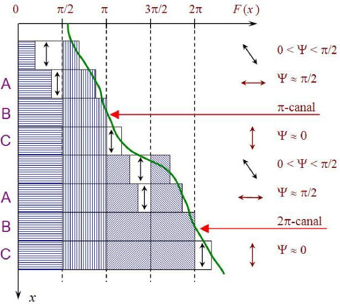
Figure 2: Diagram showing how canals are formed by differential Faraday rotation. The observer is on the right and $x$ is oriented perpendicular to their line of sight; each horizontal strip represents one telescope beam. The Faraday depth varies in the plane of the sky (with $x$) as shown with thick solid line; the intrinsic polarization angle is uniform (vertical double arrows on the left). Emission generated on the $x$-axis cancels the emission generated in a layer where the former is rotated by $\pi/2$, i.e., where $F(x)=\pi/2$. Layers whose emissions mutually cancel are indicated by perpendicularly hatched boxes. Only the emission from unshaded layers reaches the observer. The arrows on the right show the observed polarization plane which has been Faraday rotated in layers to the right of the visible (unshaded) layer to give the polarization angle $\Psi$ in the range indicated. Note that layers to the right of the ‘source’ (an unshaded layer) act as a Faraday screen, and so the rotation angle is equal to $F$. The canals occur where the polarized emission is fully cancelled (regions labelled B). The emission observed at values of $F(x)$ slightly smaller than $n\pi$ (regions A) and slightly larger than $n\pi$ (regions C) originates in different layers. The difference in $F(x)$ between regions A and C is $\pi/2$. Therefore, emission from region A is rotated by $\pi/2$ before reaching the observer, whereas emission from region C is rotated only slightly. Thus, the polarization angles observed on the two sides of a canal differ by $\pi/2$. A canal that occurs when $F(x)=n\pi$ with $n=1$ is shown near the top, and with $n=2$, near the bottom. (Adapted from Shukurov & Berkhuijsen [2003].)

If linearly polarized emission undergoes Faraday rotation, the photons originating at different positions along a single line of sight will suffer different rotations of their polarization planes. So even if all the photons are emitted with the same polarization plane, and the amount of Faraday rotation per unit path length is constant, the emerging radiation will comprise a mixture of polarization angles and the resulting degree of polarization will be reduced. This process is called differential Faraday rotation (Fig. 2); the depolarizing effect is wavelength-dependent but occurs even for infinitely small telescope beams.

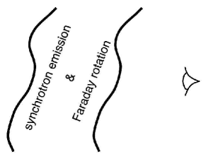
(a) Differential Faraday rotation

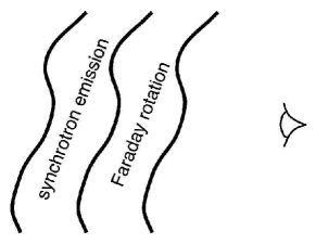
(b) Faraday screen

Figure 3: The relative positions, along the line of sight, of the regions producing synchrotron emission and Faraday rotation. The observer is on the right. (a): the case of differential Faraday rotation, , both emission and rotation occur in the same region. (b): a Faraday screen, where all the emission is produced behind the rotating layer.

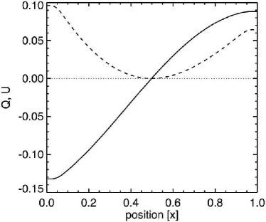
(a) Differential Faraday rotation

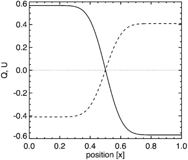
(b) Faraday screen

Figure 4: Variation of $Q$ (solid) and $U$ (dashed) (in arbitrary units) across depolarization canals caused by differential Faraday rotation (a) and in a nonuniform Faraday screen (b). In each panel, the canal occurs at $x=X_{\mathrm{c}}=0.5$ where $Q=U=0$. In Panel (a), the beam is infinitely narrow and the Faraday depth varies linearly with $x$ smoothly passing through $F=\pi$ at $x=0.5$. For the Faraday screen, the beam is a Gaussian of FWHM $D=0.2$, with the Faraday depth changing discontinuously by $\Delta F={\textstyle{\frac{1}{2}}}\pi$ at $x=0.5$. The Stokes parameters $Q$ and $U$ were obtained from Eqs. (1)–(5) for the respective configurations shown in Fig. 3 with $\epsilon,\ n_{\mathrm{e}}B_{z}$ and $\psi_{0}$ uniform along the line of sight.

Although the effect appears rather simple to understand, one can discover unexpected subtleties from simple mathematical analysis. Consider a slab extending between $-h<z<h$ along the line of sight, with constant synchrotron emissivity, $\epsilon=\mbox{const}$, and uniform magneto-ionic medium, $n_{\mathrm{e}}B_{z}=\mbox{const}$, throughout as shown in Fig. 3(a). The telescope beam is assumed to be infinitely narrow for simplicity, i.e. $W$ is a $\delta$-function in $x,y$; this makes trivial integration in the sky plane in Eq. (1). Equation (4) then yields

$$\phi(z)=\left\{\begin{array}[]{ll}F\;,&z<-h\;,\\ {\textstyle{\frac{1}{2}}}F(1-z/h)\;,&|z|\leq h\;,\\ 0\;,&z>h\;,\end{array}\right.$$ (6)

where $F=2K\lambda^{2}n_{\mathrm{e}}B_{z}$ is the Faraday depth of the slab. Then, for $\psi_{0}=\mathrm{const}$, Eqs. (1) and (3) lead to the well known result (Burn [1966])

$$\mathcal{P}=p_{0}\,\frac{\sin{F}}{F}\,\exp{\left[2i\left(\psi_{0}+{\textstyle{\frac{1}{2}}}F\right)\right]}.$$ (7)

To see more clearly how differential Faraday rotation produces depolarization canals, it is useful to rewrite this with the help of Eqs. (2) and (5):

$$p = p_{0}\left|\frac{\sin{F}}{F}\right|,$$ (8)

$$\frac{Q}{I} = p_{0}\frac{\sin{F}}{F}\cos{2(\psi_{0}+{\textstyle{\frac{1}{2}}}F)},$$ (9)

$$\frac{U}{I} = p_{0}\frac{\sin{F}}{F}\sin{2(\psi_{0}+{\textstyle{\frac{1}{2}}}F)}.$$ (10)

Equation (8) shows that $p=0$ where $|F|=n\pi$, $n=1,2\dots$. If $F$ is a continuous function of position with well-behaved contours, canals will develop on the contours of $F$ where $|F|=n\pi$. Therefore, for a canal produced by differential rotation we know the magnitude of the Faraday depth along the canal (up to an integer factor $n$). Techniques for retrieving further information about the physical state of the ISM from the statistical properties of these contours is discussed in Section 3.1.

We are free to measure the polarization angle from a line perpendicular to the transvese magnetic field near the canal; then $\psi_{0}=0$. Equations (9) and (10) show that in this reference frame

$$Q\propto\sin{F}\,\cos{F}\;,\qquad U\propto\sin^{2}{F}\;.$$

When $F(\mathbf{x})$ passes through an integer multiple of $\pi$, both $Q$ and $U$ vanish to produce a canal, but $Q$ will change sign across the canal and $U$ will not. In other words, there is always a reference frame in the sky plane such that one of the Stokes parameters changes sign, but the other does not across a canal produced by differential Faraday rotation. This behaviour is illustrated in Fig. 4(a) and we will see in Section 2.2 that this does not occur in the case of canals formed in a Faraday screen as illustrated in Fig. 4(b).

For the signs of $Q$ and $U$ shown in Fig. 4(a), $\Psi$ is in the second quadrant to the left of the canal and in the first quadrant on the right of it. As $Q\to 0$ and $U\to 0$ for $x\to X_{\mathrm{c}}$, where $X_{\mathrm{c}}$ is the position of the canal, we have $\Psi=-\pi/2$ for $x=X_{\mathrm{c}}-0$ but $\Psi=\pi/2$ for $x=X_{\mathrm{c}}+0$ — see also Eq. (5). Thus the polarization angle changes discontinuously across the canal although the magneto-ionic medium is perfectly continuous. In particular, $\mathrm{RM}$ has the same values on both sides of a canal (but is undefined at it). As illustrated in Fig. 2, the jump of the polarization angle in a continuous medium occurs because the polarized photons detected on the either side of the canal originate at different depths in the source and therefore have experienced different amounts of Faraday rotation.

The discussion above refers to the case of an infinitely narrow telescope beam; these canals are infinitely narrow curves in the sky plane. The effect of a finite beam width is twofold. Firstly, the canals in observed maps will be one beam wide, as the telescope combines emission from either side of the contour where $|F|=n\pi$. Secondly, the canals will gradually fill up with polarized emission as the resolution coarsens, so that asymmetry of the magneto-ionic medium within the beam becomes noticeable.

Canals are also filled up if the synchrotron emissivity varies along the line of sight provided this variation is not compensated by a variation in Faraday rotation. It can be shown, in particular, that a double-layered source where synchrotron intensities produced in each layer are $I_{1}$ and $I_{2}$, with $|I_{1}-I_{2}|/I_{1}=\varepsilon$, and $F=n\pi$, will produce a partially filled canal with the fractional polarization $p/p_{0}\simeq\varepsilon/\pi$, valid for $\varepsilon\ll 1$, , for weak inhomogeneity. This effect can explain why the observed canals are not all closed curves as might be expected of contours of a continuous function.

Tangled magnetic fields and fluctuations of the electron number density can produce additional depolarization known as internal Faraday dispersion, characterized by the standard deviation of the Faraday depth, $\sigma_{F}$. This effect also fills up a canal, so that the minimum fractional polarization is $p/p_{0}\simeq\sigma_{F}^{2}/\pi$ for $\sigma_{F}^{2}\ll\pi$. The above two effects are discussed by Fletcher & Shukurov (in preparation).

Joint action of various depolarization effects can produce counter-intuitive effects. For example, Sokoloff et al. ([1998], their Sect. 6.2 and Fig. 5 in Erratum) show that internal Faraday dispersion combined with differential Faraday rotation can lead to a jump of $90^{\circ}$ in polarization angle whilst the degree of polarization varies smoothly and $p$ differs from zero (if observed with infinitely narrow beam); this would appear as a canal when observed at finite resolution because of the jump in the polarization angle.

The position of a canal produced by differential Faraday rotation must change with the wavelength at which it is observed because $F$ depends on $\lambda$ according to Eq. (4). To a first approximation, a change of wavelength from $\lambda$ to $\lambda^{\prime}=\lambda+\delta\lambda$ will displace the canal by $\delta x$ where

$$\delta x\simeq\left|\frac{\delta F}{|\nabla F|}\right|\;,\qquad\delta F=F(\lambda^{\prime})-F(\lambda),\qquad|\delta\lambda|\ll\lambda\;.$$

For example, if differential Faraday rotation is the only depolarization mechanism, we have $F=2\mathrm{RM}\,\lambda^{2}$ with $\mathrm{RM}$ being independent of $\lambda$, and then

$$\delta x\simeq 2L_{\mathrm{RM}}\left|\frac{\delta\lambda}{\lambda}\right|\;,\qquad L_{\mathrm{RM}}=\left|\frac{\mathrm{RM}}{|\nabla\mathrm{RM}|}\right|\;,$$

where $L_{\mathrm{RM}}$ is the scale at which $\mathrm{RM}$ varies. Shukurov & Berkhuijsen ([2003]) argue, using a similar estimate, that the displacement can be difficult to observe if $|\delta\lambda|\;\raise 1.29167pt\hbox{$<$\kern-7.5pt\raise-4.73611pt\hbox{$\sim$ }}\;\hskip-2.0pt\lambda$, which is often the case.

2.2 Foreground Faraday screens

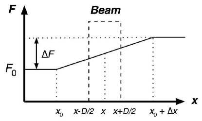
Figure 5: Sketch showing the variation of Faraday depth $F$ across the sky, here along $x$. There is a constant gradient of $F$ in the range $x_{0}<x<x_{0}+\Delta x$, and the telescope beam has a width $D$.

If synchrotron emission and Faraday rotation occur in distinct layers — with the rotating layer nearer to the observer as illustrated in Fig. 3(b) — the foreground magneto-ionic medium is called a Faraday screen. If Faraday rotation in the screen is uniform across a telescope beam then no depolarization occurs; the polarization angle of radiation emerging from the emitting layer is rotated by $\Delta\Psi=F$, but the mixing of different angles within a beam, that causes depolarization, does not occur. A Faraday screen can only cause depolarization if it is nonuniform on the scale of the beam, so that different lines of sight within the beam undergo differing amounts of Faraday rotation.

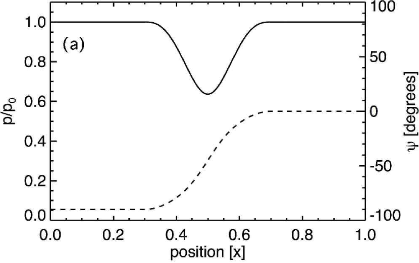
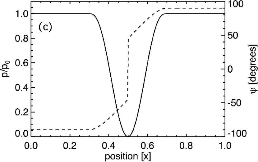
5

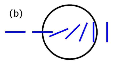
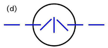
Figure 6: The variation of the fractional polarization and polarization angle across a Faraday screen with a smooth variation of Faraday depth described in Fig. 5 with $x_{0}=0.4$, $\Delta x=0.2$ and $X_{\mathrm{c}}=0.5$. Left-hand panels: (a) the change in the beam-averaged degree of polarization (solid) and polarization angle (dashed) for $\Delta F=\pi/2$ convolved with a square beam of width $D=0.2$. The fractional polarization does not reduce to zero although $\Psi$ changes by $\pi/2$ across the region. The reason is illustrated in panel (b) where we show the change in the polarization angles obtained along individual lines of sight (dashes) within the beam (circle). It is clear that the polarization cannot drop to zero in this configuration. The right-hand panels show the same as on the left, except that here $\Delta F=\pi$. Now, panel (c) shows that the fractional polarization does drop to zero at $x=X_{\mathrm{c}}$ producing a canal, but the corresponding change in $\Psi$ across the canal is $\pi$. Panel (d) explains how this variation in $\Psi$ among individual lines of sight leads to the complete depolarization. The calculation used Eqs. 1–5 for the configuration of Fig. 5.

Consider a uniform polarized radio source shining through a Faraday rotating layer. Consider a simple variation of the Faraday depth in the sky plane shown in Fig. 5, where $F$ changes by $\Delta F$ across a distance $\Delta x$, and the width of the telescope beam is $D$. We assume that the telescope beam has a square profile for simplicity. In the regions where $F=\mathrm{const}$ in Fig. 5, Eq. (1) reduces to

$$\mathcal{P}=p_{0}\left\{\begin{array}[]{ll}\exp[2i(\psi_{0}+F_{0})]\;,&x<x_{0}-D/2\;,\\ \exp[2i(\psi_{0}+F_{0}+\Delta F)]\;,&x>x_{0}+\Delta x+D/2\;,\end{array}\right.$$ (11)

so $p=\mathrm{Re}\,\mathcal{P}=p_{0}$ and no depolarization occurs if $F$ is constant. In the region $x_{0}+D/2<x<x_{0}-D/2+\Delta x$, where $F$ varies linearly, Eq. (1) yields

$$\mathcal{P} = p_{0}\exp[2i(\psi_{0}+F_{0})]\frac{1}{D}\int^{x+D/2}_{x-D/2}\exp{\left(2i\Delta F_{D}\frac{x-x_{0}}{D}\right)}\,\mathrm{d}x$$ (12)

$$= p_{0}\,\frac{\sin{\Delta F_{D}}}{\Delta F_{D}}\,\exp{[2i(\psi_{0}+F)]}\;,$$

where $\Delta F_{D}=D\,\mathrm{d}F/\mathrm{d}x$ is the increment in the Faraday depth across the telescope beam arising from a continuous gradient in $F$. (We ignore, for simplicity, the ranges $|x-x_{0}|<D/2$ and $|x-x_{0}+\Delta x|<D/2$ with a mixture of constant $F$ and a gradient in $F$ within a beam.) Then

$$p=p_{0}\left|\frac{\sin{\Delta F_{D}}}{\Delta F_{D}}\right|.$$ (13)

Thus, the depolarization in a continuously inhomogeneous screen is complete if $|\Delta F_{D}|=n\pi$ and we can then expect a canal to form along a contour where $|\nabla F|=n\pi/D$ (where we have replaced $\mathrm{d}F/\mathrm{d}x$ by $\nabla F$). An increment of $|\Delta F_{D}|=n\pi$ across the beam means that the change in polarization angle across the canal is $\Delta\Psi=180^{\circ},$ , no change — see Eq. 12. However, canals attributed to a Faraday screen by Haverkorn et al. ([2000]) have $\Delta\Psi=90^{\circ}$. As we illustrate in Fig. 6, this change in $\Psi$ in fact cannot produce a canal if $F$ varies continuously: a gradient in $F$ that produces a $90^{\circ}$ change in polarization angle across the beam does not lead to complete depolarization, whereas a gradient that produces $180^{\circ}$ of Faraday rotation does give $p=0$. Canals with $\Delta\Psi=0$ (or $180^{\circ}$) predicted here have not yet been observed.

Depolarization can be complete if the change in Faraday rotation within the beam produces a mixture of polarization angles that exactly cancel each other. Complete cancellation depends on both the variations in the Faraday depth across the screen $\Delta F$ and the telescope resolution, so that the pattern of canals can change very significantly if observed at different resolution.

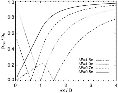
Figure 7: The minimum degree of polarization produced by a gradient of the Faraday depth in a foreground screen, $p_{\mathrm{min}}$, as a function of the relative extent of the gradient $\Delta x/D$, where $D$ is the width of a square beam. Different curves represent different Faraday rotation increments ($\Delta F$, shown in legend). For $\Delta x/D<1$, $F$ varies over a range narrower than the beam width, and is effectively discontinuous when $\Delta x/D\ll 1$. Complete depolarization in a discontinuous screen, $\Delta x/D\to 0$, occurs if $\Delta F=(2n+1)\pi/2,\ n=0,1,\ldots$.

Figure 7 shows how the depth of a canal produced by a Faraday screen depends on the increment in Faraday depth across the beam $\Delta F_{D}$ and on how well resolved this increment is, $\Delta x/D$. We can see that all gradients in $F$ can produce $p=0$ if observed at an appropriate resolution and so we should expect to see canals with all jumps in polarization angle across them. The only condition for that is that the total variation in $F$ available exceeds $\pi/2$, the minimum that can produce a canal for $\Delta x/D\ll 1$. The jump in $\Psi$ across the canal (which is one beam wide) in Fig. 7 is equal to the corresponding value of $\Delta F$ (shown in the legend) if $\Delta x/D\leq 1$ and to $\Delta F_{D}$ otherwise.

It is evident from Fig. 7 that the only way that canals with $\Delta\Psi=90^{\circ}$ will be preferentially created is if the variations in $F$ in the Faraday screen are discontinuous. In this case complete cancellation will only occur if all of the polarization angles within a beam are a mixture of exactly orthogonal pairs and canals will be formed along contours where $\Delta F_{D}=(2n+1)\pi/2$. Like the case of differential Faraday rotation, canals produced by discontinuities in a Faraday screen do not depend on the resolution of the observations. In Section 3.2 we will discuss how the statistical properties of canals formed by discontinuities in a Faraday screen can provide information about the shock-wave turbulence in the diffuse ISM.

For a canal produced by a discontinuous change of $\Delta F$, the behaviour of $Q$ and $U$ across the canal can obtained from Eq. (11) with $\Delta F=(2n+1)\pi/2$: each changes by $\pi$ (neglecting $2n\pi$ in the arguments of $\cos$ and $\sin$),

$$\frac{Q}{I}=p_{0}\left\{\begin{array}[]{ll}\cos{[2(\psi_{0}+F_{0})]},&x<X_{\mathrm{c}}\;,\\ \cos{[2(\psi_{0}+F_{0})+\pi]},&x>X_{\mathrm{c}}\end{array}\right.$$ (16)

and likewise for $U$. Figure 4 shows an example of how $Q$ and $U$ change across a canal produced in a Faraday screen and by differential Faraday rotation. In contrast to the case of differential Faraday rotation, Eqs. (9) and (10), both $Q$ and $U$ of Eq. 16 will always change sign across a canal produced by a Faraday screen. (A special case is where $Q$ (or $U$) is zero whereas $U$ (or $Q$) changes sign at the canal.) This offers an opportunity to reveal the nature of an observed canal from a careful analysis of the variation of $Q$ and $U$ across it.

3 What can we learn about the ISM from depolarization canals?

If the mechanism which forms a canal can be identified — for example by looking at the variation of $Q$ and $U$ across the canal — we then know the location of level lines of Faraday depth where $|F|=n\pi$, in the case of differential rotation, or the projected position of discontinuities with $|\Delta F_{D}|=(2n+1)\pi/2$, for the action of a Faraday screen. In both cases, canals represent contours of a random function of position in the plane of the sky, namely the Faraday depth or the magnitude of its gradient. In this section we discuss how statistical properties of the contours of a random function can be used to measure its parameters, and hence how statistical properties of the depolarization canals can be interpreted in terms of the properties of the random (turbulent) ISM.

3.1 Differential Faraday rotation: contour statistics and turbulence

As we show here, the mean separation of the contours of a differentiable random function is sensitive to the curvature of its autocorrelation function at zero lag, i.e., to a parameter known as the Taylor microscale in turbulence theory. Reviews of this theory can be found in Longuet-Higgins ([1957]), Sveshnikov ([1966]) and Vanmarcke ([1983]). Observations of canals (or contours of another observable), obtained under quite a modest resolution, provide a possibility to measure the Taylor microscale, related to the dissipation scale of the turbulent flow and to the Reynolds number. Contour statistics have been used in astrophysics in the studies of structure formation (Peebles [1984]; Barden et al. [1986]; Ryden [1988]; Ryden et al. [1989]) and the cosmic microwave background (Coles & Barrow [1987]).

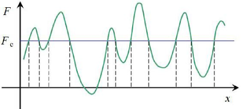
Figure 8: Crossings of a level $F_{\mathrm{c}}$ by a random function $F(x)$ are indicated with vertical dashed lines.

3.1.1 Overshoots of a random function in one dimension

We start with crossings of a random function of a single variable over a reference level (Fig. 8); a clear and detailed discussion of this problem can be found in §9 of Sveshnikov ([1966]). Consider a stationary, differentiable random function of position $\mathcal{F}(x)$, whose realisation, or measured value, is denoted by $F(x)$. (We have in mind applications where $F$ can be the Faraday depth or the magnitude of its gradient.) The function will pass, from below, through the level $F_{\mathrm{c}}$ in the infinitesimal interval $(x,x+\mathrm{d}x)$ if the following inequalities are satisfied simultaneously: $\mathcal{F}(x)<F_{\mathrm{c}}$ and $\mathcal{F}(x+\mathrm{d}x)>F_{\mathrm{c}}$. For a continuous $\mathcal{F}(x)$, we can write $\mathcal{F}(x+\mathrm{d}x)\approx\mathcal{F}(x)+\mathcal{F}^{\prime}(x)\,\mathrm{d}x$, where $\mathcal{F}^{\prime}=\mathrm{d}\mathcal{F}/\mathrm{d}x$. Thus we have

$$F_{\mathrm{c}}-\mathcal{F}^{\prime}(x)\,\mathrm{d}x<\mathcal{F}(x)<F_{\mathrm{c}}\quad\mbox{for }\mathcal{F}^{\prime}(x)>0\;.$$ (17)

In order to calculate the probability that these two inequalities hold, consider the joint probability density of $\mathcal{F}$ and its derivative $\mathcal{F}^{\prime}$ at a given position $x$, which we denote $f(F,F^{\prime})$. Then the probability of a overshoot above a level $F_{\mathrm{c}}$ is given by

$$P\{F_{\mathrm{c}}-\mathcal{F}^{\prime}(x)\,\mathrm{d}x<\mathcal{F}(x)<F_{\mathrm{c}}\}=\int_{0}^{\infty}\mathrm{d}F^{\prime}\int_{F_{\mathrm{c}}-F^{\prime}(x)\,\mathrm{d}x}^{F_{\mathrm{c}}}\mathrm{d}F\,f(F,F^{\prime})\;,$$

where integrations are performed over all values of $\mathcal{F}$ and $\mathcal{F}^{\prime}$ that satisfy Eq. (17). The integral over $F$ is immediately taken using the mean value theorem:

$$\int_{F_{\mathrm{c}}-F^{\prime}(x)\,\mathrm{d}F}^{F_{\mathrm{c}}}f(F,F^{\prime})\,\mathrm{d}x=f(F_{\mathrm{c}},F^{\prime})F^{\prime}\,\mathrm{d}x\;,$$

and then

$$P\{F_{\mathrm{c}}-\mathcal{F}^{\prime}(x)\,\mathrm{d}x<\mathcal{F}(x)<F_{\mathrm{c}}\}=\mathrm{d}x\int_{0}^{\infty}f(F_{\mathrm{c}},F^{\prime})F^{\prime}\,\mathrm{d}F^{\prime}\;.$$ (18)

It is convenient to introduce the probability density of an overshoot, , the probability $p_{\mathrm{a}}(F_{\mathrm{c}})$ of an overshoot above a level $F_{\mathrm{c}}$ at a position $x$ per unit interval of $x$. The above result can be written as

$$p_{\mathrm{a}}(F_{\mathrm{c}})=\int_{0}^{\infty}f(F_{\mathrm{c}},F^{\prime})\,F^{\prime}\,\mathrm{d}F^{\prime}\;.$$

Similarly, we obtain the probability density for $F(x)$ to cross the level $F_{\mathrm{c}}$ from above:

$$p_{\mathrm{b}}(F_{\mathrm{c}})=-\int_{-\infty}^{0}f(F_{\mathrm{c}},F^{\prime})\,F^{\prime}\,\mathrm{d}F^{\prime}\;,$$

and the total probability density for $F(x)$ to cross the level $F_{\mathrm{c}}$ at a position $x$ either from above or from below is given by

$$p_{\mathrm{c}}=p_{\mathrm{a}}+p_{\mathrm{b}}=\int_{-\infty}^{\infty}f(F_{\mathrm{c}},F^{\prime})\,|F^{\prime}|\,\mathrm{d}F^{\prime}\;.$$ (19)

It can be shown (Sveshnikov [1966]) that the mean numbers of crossings of a level $F_{\mathrm{c}}$ per unit length, $N_{1}$, is equal to $p_{\mathrm{c}}$, , the mean separation of the crossing points is given by

$$\overline{x}_{\mathrm{c}}=N_{1}^{-1}=p_{\mathrm{c}}^{-1}\;,$$

where overbar denotes averaging.

The results can be written in a closed, explicit form if $\mathcal{F}(x)$ is a Gaussian random function because then the fact that $\mathcal{F}(x)$ and $\mathcal{F}^{\prime}(x)$ are uncorrelated (which is true for any stationary, differentiable random function) implies that they are statistically independent, so that

$$f(F,F^{\prime})=f_{F}(F)f_{F^{\prime}}(F^{\prime})\;,$$

and hence (we note that $\overline{F^{\prime}}=0$)

$$f(F,F^{\prime})=\frac{1}{\sigma_{F}(2\pi)^{1/2}}\,\exp{\left[-\frac{(F-\overline{F})^{2}}{2\sigma_{F}^{2}}\right]}\,\frac{1}{\sigma_{F^{\prime}}(2\pi)^{1/2}}\,\exp{\left[-\frac{(F^{\prime})^{2}}{2\sigma_{F^{\prime}}^{2}}\right]}\;,$$

where we have introduced the standard deviations of $F$ and $F^{\prime}$, $\sigma_{F}$ and $\sigma_{F^{\prime}}$, respectively. Integration over $F^{\prime}$ in Eq. (19) can now be easily performed to obtain

$$N_{1}=p_{\mathrm{c}}=\frac{1}{\pi}\,\frac{\sigma_{F}}{\sigma_{F^{\prime}}}\exp{\left[-\frac{(F_{\mathrm{c}}-\overline{F})^{2}}{2\sigma_{F}^{2}}\right]}.$$ (20)

In application to canals, where $F_{\mathrm{c}}=n\pi,\ n=1,2,\ldots$ in the case of differential Faraday rotation, one needs to calculate the mean separation of positions where $|F(x)|=F_{\mathrm{c}}$. The corresponding probability density involves an additional contribution arising from crossings at $F(x)=-F_{\mathrm{c}}$, which should be added to the right-hand side of Eq. (20). The additional term is proportional to $\exp[-(F_{\mathrm{c}}+\overline{F})^{2}/2\sigma_{F}^{2}]$. This term can be significant if $\overline{F}\approx 0$, so that $|F_{\mathrm{c}}-\overline{F}|\simeq|F_{\mathrm{c}}+\overline{F}|$. If only one of the two terms is significant, it is sufficient to replace $\overline{F}$ by $|\overline{F}|$ in Eq. (20).

Since

$$\frac{\sigma_{F^{\prime}}^{2}}{\sigma_{F}^{2}}=-\left.\frac{\mathrm{d}^{2}C(r)}{\mathrm{d}r^{2}}\right|_{r=0}=\frac{2}{l_{\mathrm{T}}^{2}}\;,$$

where $C(r)$ is the autocorrelation function of $F(x)$ normalised to $C(0)=1$ and $l_{\mathrm{T}}$ is known as the Taylor microscale (e.g., Sect. 6.4 in Tennekes & Lumley [1972]), we obtain the following expression for the mean separation of the positions where $|F(x)|=F_{\mathrm{c}}$:

$$\overline{x}_{\mathrm{c}}=\frac{\pi}{\sqrt{2}}\,l_{\mathrm{T}}\,\exp{\left[\frac{(F_{\mathrm{c}}-|\overline{F}|)^{2}}{2\sigma_{F}^{2}}\right]}\;.$$ (21)

3.1.2 Contour statistics in two dimensions

The theory of overshoots can be generalized to two dimensions, where we consider a random field $\mathcal{F}(\mathbf{x})$ depending on two variables $\mathbf{x}=(x,y)$ (e.g., position in the sky plane); we also introduce $\mathbf{V}=\nabla\mathcal{F}$. The probability of an overshoot is now equal to the probability that the following inequalities are satisfied simultaneously:

$$\mathcal{F}(\mathbf{x})<F_{\mathrm{c}}\;,\qquad\mathcal{F}(\mathbf{x}^{\prime})>F_{\mathrm{c}}\;,\qquad\mathbf{x}^{\prime}=\mathbf{x}+\mathrm{d}\mathbf{x}\;,$$

where $\mathrm{d}\mathbf{x}=\widehat{\mathbf{V}}\,\mathrm{d}x$, with $\widehat{\mathbf{V}}=\nabla\mathcal{F}/|\nabla\mathcal{F}|$ the unit vector parallel to the gradient of $\mathcal{F}$. Expanding $\mathcal{F}(\mathbf{x}^{\prime})\approx\mathcal{F}(\mathbf{x})+\nabla\mathcal{F}\cdot\mathrm{d}\mathbf{x}$ and retaining only the term linear in $\mathrm{d}\mathbf{x}$, we reduce the above inequalities to

$$F_{\mathrm{c}}-|\nabla\mathcal{F}(\mathbf{x})|\,\mathrm{d}x<\mathcal{F}(\mathbf{x})<F_{\mathrm{c}}\;,$$

and, using arguments similar to those that lead to Eq. (18) and further, we obtain the probability of a crossing (either upward or downward) of the contour $\mathcal{F}(\mathbf{x})=F_{\mathrm{c}}$ in two dimensions:

$$p_{\mathrm{c}}^{(2)}=\int_{-\infty}^{\infty}\int_{-\infty}^{\infty}f(F_{\mathrm{c}},\mathbf{V})\,|\mathbf{V}|\,\mathrm{d}V_{x}\,\mathrm{d}V_{y}\;$$

where $f(F_{\mathrm{c}},\mathbf{V})$ is the joint probability distribution of $\mathcal{F}$ and its gradient. This quantity can be identified with the mean length of the $F_{\mathrm{c}}$ contour per unit area,

$$N_{2}=p_{\mathrm{c}}^{(2)}\;.$$

In both one and two dimensions, the probability of crossing a contour is given by the mean value of the magnitude of the gradient of the random field at that contour. As discussed by Ryden ([1988]), for an isotropic random field $\mathcal{F}$, the mean number of crossings per unit length along a line, $N_{1}$, and the mean length of a contour per unit area, $N_{2}$, are related,

$$N_{2}=\frac{\pi}{2}N_{1}\;,$$

and so statistical properties of contours in the plane can be conveniently studied using one-dimensional cuts, which is technically easier.

3.1.3 The separation of canals and parameters of ISM turbulence

Shukurov & Berkhuijsen ([2003]) applied a one-dimensional version of this theory to canals observed at $\lambda 20.5\,\mathrm{cm}$ in the direction to the Andromeda nebula (around $l=120^{\circ},b=-20^{\circ}$). Their estimate of the mean separation of canals is $5^{\prime}$ which results in a estimate of the Taylor microscale of RM (or, more precisely, the Faraday depth) of $l_{\mathrm{T}}\simeq 2^{\prime}$. For the presumed mean distance within the Milky Way’s non-thermal disc in that direction, 1 kpc, the corresponding linear scale is 0.6 pc. If this scale can be identified with the Taylor microscale of interstellar turbulence (which may or may not be the case!), the effective value of the Reynolds number follows as $\mathrm{Re}\simeq(l_{0}/l_{\mathrm{T}})^{2}\simeq 10^{5}$ for the energy-range scale of $l_{0}=100\,\mathrm{pc}$. This value of Re is many orders of magnitude smaller than those based on the molecular viscosity. If this estimate can be confirmed by more comprehensive and deeper analyses, this would imply that the dissipation range of the interstellar MHD turbulence is controlled by relatively large viscosities, perhaps associated with kinetic plasma effects. The latter are often described as anomalous viscosity or resistivity; useful recent results were obtained in the context of galaxy clusters by Schekochihin et al. ([2005]).

3.2 Faraday screens: the mean separation of canals and shocks

If canals are caused by rotation measure discontinuities in a Faraday screen, the mean distance between them will be related to the distribution of discontinuities in the ISM. Most plausibly these are shock fronts. (Another possible source are tangential discontinuities but it is difficult to identify a physical reason for their widespread occurrence.)

A canal forms where the background Faraday depth $F$ changes by $|\Delta F|=(n+1/2)\pi$ across a shock front. If the magnetic field is frozen into the gas and the gas density increases by a factor $\epsilon_{\rho}$ then so will the field strength (we neglect a factor $\sim 1/\sqrt{2}$ due to the relative alignment of the shock and field). Therefore

$$\epsilon_{\rho}\simeq\sqrt{\left|\frac{\Delta F}{F_{0}}\right|+1}.$$ (22)

The increase in gas density depends on the Mach number of the shock $\mathcal{M}$ as (e.g. Landau & Lifshitz [1960])

$$\epsilon_{\rho}=\frac{(\gamma+1)\mathcal{M}^{2}}{(\gamma-1)\mathcal{M}^{2}+2}\simeq 4\frac{\mathcal{M}^{2}}{\mathcal{M}^{2}+3}$$ (23)

where we have used $\gamma\simeq 5/3$ for the polytropic index of the gas. Combining Eqs. (22) and (23), we obtain the minimum Mach number necessary to produce a canal,

$$\mathcal{M}_{*}\simeq\sqrt{\frac{3\epsilon_{\rho}}{4-\epsilon_{\rho}}}=\left[\frac{4}{3(|\Delta F/F_{0}|+1)^{1/2}}-\frac{1}{3}\right]^{-1/2},\hskip 14.22636pt|\Delta F|=\frac{\pi}{2}.$$ (24)

As follows from Sect. 2.2, stronger shocks can also produce canals.

The dominant source of the primary shocks are supernovae. When these shocks encounter gas clouds they will be reflected, generating a population of secondary shocks. Following Bykov & Toptygin ([1987]), the probability density function of both primary and secondary shocks is given by

$$G(\mathcal{M})\simeq G_{0}\left[\frac{1}{\mathcal{M}^{\alpha+1}}+\frac{3C(\alpha)f_{\mathrm{cl}}}{(\mathcal{M}-1)^{4}}\right],$$ (25)

where $G_{0}=S\frac{4}{3}\pi r_{0}^{3}$, $S$ is the supernova rate per unit volume, $r_{0}$ is the maximum radius of a supernova (primary) shock, and $\alpha$ characterizes the dependence of the shock radius on the Mach number, $r(\mathcal{M})=r_{0}\mathcal{M}^{-\alpha/3}$, $f_{\mathrm{cl}}$ is the volume filling factor of diffuse clouds and $C(\alpha)$ is a constant. For the Sedov solution, $\alpha=2$ and for a three-phase ISM, $\alpha=4.5$; $C(\alpha)=2.3\times 10^{-2}$ for $\alpha=2$ and $4.1\times 10^{-3}$ for $\alpha=4.5$. The mean number of shocks of a strength $\geq\mathcal{M}$ crossing a position in the ISM per unit time is

$$H(\mathcal{M})=\int_{\mathcal{M}}^{\infty}G(\mathcal{M})\,\mathrm{d}\mathcal{M}=G_{0}\left[\frac{1}{\alpha\mathcal{M}^{\alpha}}+\frac{C(\alpha)f_{\mathrm{cl}}}{(\mathcal{M}-1)^{3}}\right],$$ (26)

and the mean separation of shocks with a strength $\geq\mathcal{M}$ is

$$L(\mathcal{M})\simeq\frac{c_{s}}{H(\mathcal{M})},$$ (27)

with $c_{s}$ the sound speed. Substituting Eqs. (24) and (26) into Eq. (27), we find the mean separation of shocks in three dimensions:

$$L \simeq 9\,\mathrm{pc}\left(\frac{c_{s}}{10\,\mathrm{km\,s^{-1}}}\right)\left(\frac{\nu_{\mathrm{SN}}}{0.02\,\mathrm{yr}^{-1}}\right)^{-1}\left(\frac{R}{15\,\mathrm{kpc}}\right)^{2}\left(\frac{h}{50\,\mathrm{pc}}\right)\left(\frac{r_{0}}{100\,\mathrm{pc}}\right)^{-3}$$ (28)

$$\mbox{}\times\left[\frac{1}{\alpha\mathcal{M}_{*}^{\alpha}}+\frac{C(\alpha)f_{\mathrm{cl}}}{(\mathcal{M}_{*}-1)^{3}}\right]^{-1},$$

where $\nu_{\mathrm{SN}}$ is the Galactic supernova rate, $R$ and $h$ are the radius and scale height of the star-forming disc respectively; the term in the square brackets is close 0.2 for $\mathcal{M}=1.2$ and $\alpha=4.5$. Projecting onto the sky plane changes $\mathcal{L}$ by a factor $\xi=\pi^{-1}\int_{0}^{\pi}\sin^{2}\theta\,\mathrm{d}\theta=1/2$. If the shocks fill a region of a depth $d$, the separation of the shocks in the plane of the sky is further reduced by a factor $d/L$. The angular separation $\mathcal{L}$ at an average distance $d/2$ to the shocks follows as

$$\mathcal{L}=\frac{L^{2}}{d^{2}}$$ (29)

As an example, let us use the observations by Haverkorn et al. ([2003]) as inputs to Eq. (29) and compare the observed separation of canals with the predicted separation of shocks. In this field the average Faraday depth is $F\simeq\pi\,\mathrm{radians}$ and the most abundant canals are produced when $|\Delta F|=\pi/2$, since weaker shocks are the most abundant according to Eq. (25). Equation (24) then gives $\mathcal{M}_{*}\simeq 1.2$. The maximum depth of the layer is estimated as $d\simeq 600\,\mathrm{pc}$. With the parameter values used to normalize Eq. (28) and $f_{\mathrm{cl}}=0.25$, $\alpha=4.5$, we obtain a mean separation of canals of $L\simeq 40\,\mathrm{pc}$, or $\mathcal{L}\simeq 15^{\prime}$. The latter value is reasonably close to a by-eye estimate of the average separation of canals in Fig. 3 of Haverkorn et al. ([2003]) of $45^{\prime}$. Thus, the canals observed by Haverkorn et al. ([2003]) are compatible with a system of shocks producing discontinuities in a Faraday screen. The canals in these observations appear to be straighter (or less twisting) than those observed at shorter wavelengths by, e.g., Uyanıker et al. ([1998b]) and Gaensleret al. ([2001]). This might be expected if the straighter canals arise from shocks in the diffuse ISM and the twisting canals have a different origin such as differential Faraday rotation. The Mach number of the shocks required to produce $|\Delta F|=\pi/2$ at metre wavelengths is quite low, so that they can be inefficient in accelerating cosmic rays. Then the expected increase in total synchrotron emissivity at a shock is just $\mathcal{M}_{*}^{2}\simeq 1.5$. Such features can be difficult to detect in total intensity radio maps, especially if their area covering factor is high.

4 Prospects

At first sight, the chaotic appearance of radio polarization maps of the diffuse Milky Way emission and the difficulty of connecting standard statistical tools, such as power spectra, to ISM physics, makes interpretation of the data a daunting task. Moreover, changes in the polarization pattern with wavelength depend on random quantities, such as the thermal electron density and magnetic field fluctuations. Analysis of the ubiquitous depolarization canals provides a practical starting point from which we can develop the methods required to make full use of the polarization observations. As we have shown here, the origin of canals can be determined from observed quantities — by examining how $Q$ and $U$ vary across a canal — and their statistical measures are related to the parameters of interstellar turbulence. The extension of methods used to study canals to the wider analysis of polarized radio emission will lead to better techniques for separating Milky Way foregrounds from polarized cosmological signals.

References

- [1986] Barden J. M., Bond J. R., Kaiser N. & Szalay A. S., 1986, ApJ, 304, 15
- [1999] Beck R., 1999, in “Galactic Foreground Polarization”, ed. E. M. Berkhuijsen (MPIfR: Bonn), p. 3
- [1966] Burn B. J., 1966, MNRAS, 133, 67
- [1987] Bykov A. M. & Toptygin N., 1987, Ap&SS, 138, 341
- [1987] Coles P. & Barrow J. D., 1987, MNRAS, 228, 407
- [1999] Duncan A. R., Reich P., Reich W. & Fürst E., 1999, A&A, 350, 447
- [1989] Eilek J. A., 1989, AJ, 98, 244
- [2001] Gaensler B. M., Dickey J. M., McClure-Griffiths N. M., Green A. J., Wieringa M. H. & Haynes R. F., 2001, ApJ, 549, 959
- [1999] Gray A. D., Landecker T. L., Dewdney P. E., Taylor A. R., Willis A. G. & Normandeau M., 1999, ApJ, 514, 221
- [2004] Haverkorn M. & Heitsch F., 2004, A&A, 421, 1011
- [2000] Haverkorn M., Katgert P. & de Bruyn A. G., 2000, A&A, 356, L13
- [2003] Haverkorn M., Katgert P. & de Bruyn A. G., 2003, A&A, 403, 1031
- [2004] Haverkorn M., Katgert P. & de Bruyn A. G., 2004, A&A, 427, 549
- [1960] Landau L. D. & Lifshitz E. M., 1960, “Fluid Mechanics” (Pergamon Press: Oxford)
- [1957] Longuet-Higgins M. S., 1957, Phil. Trans. R. Soc. London, Ser. A, 249, 321
- [1984] Peebles P. J. E., 1984, ApJ, 277, 470
- [2004] Reich, W., Fürst, E., Reich, P., Uyanıker, B., Wielebinski, R. & Wolleben, M., 2004, in “The Magnetized Interstellar Medium”, ed. B. Uyanıker, W. Reich & R. Wielebinski (Katlenburg-Lindau: Copernicus), p. 45
- [1988] Ryden B. S., 1988, ApJ, 333, L41
- [1989] Ryden B. S., Melott A. L., Craig D. A., Gott R., Weinberg D. H., Scherrer R. J., Bhavsar S. P. & Miller J. M., 1989, ApJ, 340, 647
- [2005] Schekochihin A. A., Cowley S. C., Kulsrud R. M., Hammett G. W. & Sharma P., 2005, ApJ, 629, 139
- [2003] Shukurov A. & Berkhuijsen E. M., 2003, MNRAS, 342, 496 (Erratum: 2003, MNRAS, 345, 1392)
- [1998] Sokoloff D. D., Bykov A. A., Shukurov A., Berkhuijsen E. M., Beck R. & Poezd A. D., 1998, MNRAS, 299, 189 (Erratum: 1999, MNRAS, 303, 207)
- [1966] Sveshnikov A. A., 1966, “Applied Methods in the Theory of Random Functions” (Pergamon Press: Oxford)
- [1972] Tennekes H., Lumley J. L., 1982, “A First Course in Turbulence” (MIT Press: Cambridge, Mass)
- [1998a] Uyanıker B., Fürst E., Reich W., Reich P. & Wielebinski R., 1998a, A&AS, 132, 401
- [1998b] Uyanıker B., Fürst E., Reich W., Reich P. & Wielebinski R., 1998b, A&AS, 138, 31
- [1983] Vanmarcke E., 1983, “Random Fields: Analysis and Synthesis” (MIT Press: Cambridge, Mass.)
- [1993] Wieringa M. H., de Bruyn A. G., Jansen D., Brouw W. N. & Katgert P., 1993, A&A, 268, 215
- [2006] Wolleben M., Landecker T. L., Reich W. & Wielebinski R., 2006, A&A, 448, 411