ESO Imaging Survey: Infrared observations of CDF-S and HDF-S

This paper presents infrared data obtained from observations carried out at the ESO 3.5m New Technology Telescope (NTT) of the Hubble Deep Field South (HDF-S) and the Chandra Deep Field South (CDF-S). These data were taken as part of the ESO Imaging Survey (EIS) program, a public survey conducted by ESO to promote follow-up observations with the VLT. In the HDF-S field the infrared observations cover an area of $\sim$ 53 square arcmin, encompassing the HST WFPC2 and STIS fields, in the $JHK_{s}$ passbands. The seeing measured in the final stacked images ranges from 0$\aas@@fstack{\prime\prime}$79 to 1$\aas@@fstack{\prime\prime}$22 and the median limiting magnitudes (AB system, 2” aperture, 5 $\sigma$ detection limit) are $J_{AB}\sim 23.0$, $H_{AB}\sim 22.8$ and $K_{AB}\sim 23.0$ mag. Less complete data are also available in $JK_{s}$ for the adjacent HST NICMOS field. For CDF-S, the infrared observations cover a total area of $\sim$ 100 square arcmin, reaching median limiting magnitudes (as defined above) of $J_{AB}\sim 23.6$ and $K_{AB}\sim 22.7$ mag. For one CDF-S field $H$ band data are also available. This paper describes the observations and presents the results of new reductions carried out entirely through the un-supervised, high-throughput EIS Data Reduction System and its associated EIS/MVM C++-based image processing library developed, over the past 5 years, by the EIS project and now publicly available. The paper also presents source catalogs extracted from the final co-added images which are used to evaluate the scientific quality of the survey products, and hence the performance of the software. This is done comparing the results obtained in the present work with those obtained by other authors from independent data and/or reductions carried out with different software packages and techniques. The final science-grade catalogs together with the astrometrically and photometrically calibrated co-added images are available at CDS.

1 Introduction

One of the goals of the ESO Imaging Survey (EIS, Renzini & da Costa, 1997) was to carry out moderately deep, multi-passband, optical/infrared observations over relatively large areas to produce faint galaxy samples. The primary objective was to produce samples with color information to estimate photometric redshifts, extract statistical samples of galaxies likely to be in the poorly sampled $1\lesssim z<2$ redshift interval or Lyman-break candidates at $z\gtrsim 2.5$ and, perhaps, examples of high redshift quasars and galaxies all of which are interesting targets for follow-up spectroscopic observations with the VLT.

The first such attempt was the EIS-DEEP survey carried out at the NTT in the period 1998-2000. The infrared part of the survey was carried out in the period 1998-1999 and is reported in the present paper. While by recent standards this survey is relatively modest in size, the combination of depth and area made it unique at the time it was conceived. The survey consisted of optical and infrared observations of the Hubble Deep Field South (HDF-S, Williams et al., 2000) and the Chandra Deep Field South (CDF-S, Giacconi et al., 2001). The choice of the regions was an attempt by the EIS Working Group to reconcile the great interest generated by the HST observations of a region selected in the southern hemisphere (HDF-S), with the desire to conduct observations in a less crowded region and, in particular, devoid of bright stars. Therefore, the second region was chosen to overlap the area, selected for its low HI column density, for which deep Chandra observations were already being planned. This region is particularly well-suited for ground-based imaging due to its lack of bright stars. Not surprisingly, it eventually became a widely explored window to the high redshift Universe with deep multi-wavelength observations being conducted by all major space observatories and several ground-based follow-up programs (e.g. Giavalisco et al., 2004).

Preliminary results of this survey were originally reported in preprints by da Costa et al. (1998) and Rengelink et al. (1998) who presented fully calibrated optical and infrared images, single-passband catalogs extracted from these images, color catalogs based on a reference $\chi^{2}$ image and lists of color-selected high-redshift galaxy candidates utilizing the Ly-break technique. All of these data products were made publicly available world-wide. The optical images were reduced using IRAF and the infrared images using the program Jitter of the Eclipse library (Devillard et al., 1999) developed by ESO to reduce ISAAC and SOFI data.

Despite satisfactory attempts to assess the quality of the derived products by, for instance, comparing counts of galaxies with those of other authors and of star counts and the stellar locus in color-color diagrams with model predictions, subsequent comparisons with deeper data and with independent analysis using other reduction techniques showed that the reductions carried out by the EIS team using the available Jitter package led to a systematic loss of flux at faint magnitudes. The color catalogs released also showed some unexpected results which, after some time, were traced to relative offsets between the astrometric calibration of the optical and infrared images. Due to these problems the abovementioned preprints were withdrawn and the data release described in the present work supersedes those made earlier by the EIS team of this dataset. The identified problems, together with the need to develop a common, high-throughput system to handle optical/infrared, single and multi-chip instruments, led to the development, as part of the EIS project, of an image processing engine (EIS/MVM library, Vandame, 2004). This library is a central part of the integrated, end-to-end EIS Data Reduction System (da Costa et al., 2004) built to carry out un-supervised image reductions, stacking and catalog preparation. Preliminary results obtained with the new image processing library, in particular addressing the flux loss problem were originally reported by Vandame et al. (2001). However, even though a significant improvement was achieved, additional testing indicated that an error was introduced in the code. To avoid additional intermediate releases, the final release of these data was postponed until the completion of the EIS Data Reduction System infrastructure which includes the photometric pipeline and provides the infrastructure required for re-processing and re-calibrating data in an efficient way, a key element for testing new software.

In this paper these new reductions of the data accumulated by EIS-DEEP, including new ones not previously released, are presented. In Sect. 2, the observations, including those carried out in 1999 and not previously reported, are reviewed. The goal of this paper is two-fold: first, provide the most recent reductions and substitute previous releases; second, use these data as a test case to justify the use of the developed software to treat the much larger dataset accumulated by the infrared part of the Deep Public Survey (DPS) carried out by the EIS team over 81 nights in the period 2000-2004, which generated about 15000 science frames. The results for this survey will be presented in a forthcoming paper of this series (Olsen et al., 2006). In Sect. 3 the procedures adopted to remove the instrumental signature and to astrometrically and photometrically calibrate the nightly data are discussed, while in Sect. 4 the attributes of the final co-added images and their associated catalogs are presented. The scientific quality of these advanced survey products is assessed by comparing in Sect. 5 the results derived from the present dataset with those obtained from a variety of other datasets reduced using diverse techniques. The main results of the present paper are summarized in Sect. 6.

2 Observations

Table 1: SOFI Pointings (J2000.0).

Field	$\alpha$	$\delta$
HDF-S-1	22:33:29.1	-60:33:50
HDF-S-2	22:32:42.4	-60:33:50
HDF-S-3	22:33:00.0	-60:37:59
CDF-S-1	03:32:16.7	-27:46:00
CDF-S-2	03:32:38.0	-27:46:00
CDF-S-3	03:32:16.7	-27:50:35
CDF-S-4	03:32:38.0	-27:50:35

Table 2: Number of observed fields in each region.

Region	$J$	$H$	$K_{s}$
CDF-S	4	1	4
HDF-S	3	2	3

As described above, the EIS-DEEP observations originally were planned to cover two regions: one region consisting of three adjacent fields, of about 25 square arcmin each, covering the WFPC2, STIS and NIC3 fields; and another region constituting a $2\times 2$ mosaic, comprising a total area of $\sim 100$ square arcmin covering part of the now well-known CDF-S region. The center of the mosaic was chosen to coincide with the nominal position selected for the X-ray observations, where the sensitivity and image quality were expected to be the best. The pointings adopted in the construction of the mosaics are listed in Table 1.

The observations were obtained using the SOFI camera (Moorwood et al., 1998) mounted on the NTT. SOFI is equipped with a Rockwell 1024² detector that, when used together with its large field objective, provides images with a pixel scale of 0.29 arcsec, and a field of view of about $4.9\times 4.9$ square arcmin. The total area covered in $J$ and $K_{s}$ is about $\sim 175$ square arcmin split into two mosaics, one of $\sim 75$ square arcmin covering HDF-S and the other of $\sim 100$ square arcmin covering CDF-S. The observations were carried out in groups of exposures (OBs). The excution of an OB consists of a series of short exposures with small position offsets from the target position. The observations were conducted using the AutoJitter observing template, which implements the offsetting of adjacent exposures within a box of a user specified size $s$, chosen to be $s=45$ arcsec, approximately 15% of the field of view. The offsets are constrained so that all distances between pointings, in a series of 15 consecutive exposures are larger than 9 arcsec. Each observation comprised sixty one-minute exposures, which themselves were the average of six ten-second sub-exposures. Table 2 summarizes the available observations for each of the mosaics. The numbers listed in the table represent the number of observed fields regardless of their exposure times.

A total of 3051 science frames were obtained. Out of those, 1316 are in the CDF-S region and represent 22 hours of on-target integration, obtained during 7 nights in the period August 3, 1998 and November 11, 1998. The remaining 1735 are located in the HDF-S region and were accumulated in 29 hours of on-target integration, in observations carried out during 14 nights over the period August 3, 1998 to July 7, 1999. Observations of standard stars are available for all nights, generating 613 images taken in 7805 sec.

3 Data reduction

The new reduction of the data, described in the present paper, was carried out using the EIS Data Reduction System (da Costa et al., 2004), which is an end-to-end, integrated system providing the infrastructure for the un-supervised reduction and calibration of large volumes of imaging data. An integral part of the reduction system is a C++-based image processing library (EIS/MVM library, Vandame, 2004) developed as part of the EIS effort. It is both a library of basic image processing routines, and an integrated, high-throughput pipeline (reaching a sustainable rate of about 0.5 Mpix/sec) for automated reduction of single or multi-chip optical/infrared images.

The main steps of the EIS Data Reduction System are: the creation of reduced images on a night by night basis; the photometric calibration of the reduced images; stacking of the reduced images yielding the final stacked images forming the basis of the catalog extraction. The EIS/MVM pipeline is responsible for the first step of producing fully reduced images and weight-maps carrying out bias subtraction, flatfielding, de-fringing, correction of eletronic cross-talk effects, identification and automatic masking of satellite tracks, and sky-background subtraction as well as first-order pixel-based image stacking (allowing for translation, rotation and stretching of the image). The stacking process combines the reduced images into final image stacks properly flux scaling the images to conserve the photometric calibration. Finally, the object catalogs are extracted using SExtractor. The reductions of optical wide-field imaging data are presented by Dietrich et al. (2005, hereafter Paper I) and Mignano et al. (2006), where details about common aspects of the reduction can be found. Paper I also includes a detailed description of the released images and catalogs and their format. Here only the more important steps for handling infrared data are reviewed.

After the basic image reduction, the de-fringing, sky-subtraction and elimination of image artifacts are carried out in a two-step procedure: first, a preliminary image is obtained by stacking a set of sky-subtracted frames, with the background estimated using a running median; second, objects are identified in this stacked image and masks are created and enlarged by a user-specified factor; finally, the de-fringing/sky-subtraction step is repeated with the object masks mapped to the jittered position of each individual image. In the final co-addition of the images the masked pixels are neglected and deviant pixels are clipped. This procedure is particularly important for infrared observations since, as explained in Sect. 2, the observations are carried out as sequences of short exposures, in order to allow a suitable estimate of the fast varying background at these wavelengths to be made. The short exposure time of the individual images, prevent the detection of a large number of objects with non-negligible flux, which can make a significant contribution to the background when several images are co-added. Therefore, if these objects are not properly masked when estimating the background, the background is over-estimated, biasing the flux of even relatively bright objects. This was the effect observed in the original release of the EIS-DEEP data using the Eclipse reduction package (da Costa et al., 1998; Rengelink et al., 1998). With the two-step procedure now adopted, the flux estimates have greatly improved and, as shown in Sect. 5, the flux estimates are in excellent agreement with those obtained using other reduction packages commonly used to reduce infrared data.

The library also includes advanced algorithms used for the astrometric calibration and warping of reduced images onto a user-defined reference grid. The astrometric calibration of the infrared frames was performed using the GSC2.2 (HDF-S) and USNO-B (CDF-S, Monet et al., 2003) catalogs as reference following the method developed by Djamdji et al. (1993). The GSC2 catalog was used because of the lack of reference stars in the USNO-B within the surveyed are of the HDF-S region. The internal astrometric accuracy is about half a pixel ($\sim$0.15 arcsec) and is limited by the internal accuracy of the reference catalog. When dealing with multi-wavelength surveys it is preferable to register the infrared data using a catalog from an optical counterpart image. This will not only provide a much larger number of reference objects but also avoid the effects associated with small deviations of the astrometric solutions obtained for the optical and infrared data that were identified in the original release of the EIS-DEEP data.

The photometric calibration for each night is based on observations of standard stars taken from Persson et al. (1998). Typically two to seven stars were observed over a range of airmass. For all nights, independent photometric solutions were attempted using the photometric pipeline of the EIS Data Reduction System. Depending on the airmass and color coverage linear fits with one, two or three free parameters are attempted. If no standard star observations are available or no suitable fits are possible a default solution is adopted. This was the case for only two nights: August 4, 1998 for both $J$ and $K_{s}$ bands and November 11, 1998 for the $K_{s}$-band with insufficient observations of standard stars during the night to derive a reliable solution.

Table 3: Type of photometric solutions available for each combination of mosaic and band.

Region	Passband	Default	1-par	2-par	3-par	total
CDF-S	$J$	0	1	2	0	3
CDF-S	$H$	0	0	1	0	1
CDF-S	$K_{S}$	1	1	2	0	4
HDF-S	$J$	1	4	0	0	5
HDF-S	$H$	0	4	0	0	4
HDF-S	$K_{s}$	1	4	1	0	6

Table 4: Average photometric solutions. There was no case where the color term could be determined.

Passband	Zp	k
$J$	$23.21\pm 0.05$	$0.11$
$H$	$23.00\pm 0.05$	$0.02$
$K_{s}$	$22.45\pm 0.06$	$0.13$

Table 5: Comparison between EIS and Telescope Team solutions (EIS-Telescope). There was no case where the color term could be determined.

Passband	Zp	k
$J$	-0.07	0.01
$H$	-0.06	-0.02
$K_{s}$	0.0	0.03

Table 3 summarizes the type of photometric solutions available for each mosaic. The table gives in Col. 1 the region name; in Col. 2 the passband; in Col. 3 the number of default solutions; in Cols. 4–6 the number of nights with photometric solutions derived from 1- to 3- parameter fits; and in Col. 7 the total number of nights with science and standard star observations for a given combination of mosaic and passband. It can be seen that in many cases only 1-parameter fits are available, in particular in the HDF-S mosaic, and that no solution was obtained with an independent estimate of the color term. This is the result of insufficient airmass and/or color coverage of the standard star observations. Note that for mosaics, in principle, one good solution suffices to determine a reliable calibration, using overlapping regions to propagate a given solution.

Table 4 summarizes the average photometric solutions determined for the entire period of observations, covering more than one year. The table lists in Col. 1 the passband; in Col. 2 the mean zeropoint and standard deviation; in Col. 3 the mean extinction. The number of solutions is in general small ranging from 1 to 6 solutions in the different bands and only for 1–3 of these could the extinction be determined, as can also be seen from Table 3. Therefore, the standard deviation for the extinction values could not be determined reliably. The errors estimated for the extinction values are typically of the order of $\lesssim 0.05$. The listed standard deviations are a good indication of the uncertainty of the estimated zeropoints. The solutions have been compared with the values provided by the Telescope Team in Table 5 listing in Col. 1 the passband; in Col. 2 the difference in zeropoint of the photometric solutions computed as (EIS-Telescope Team); in Col. 3 the corresponding difference for the determined extinction. It can be seen that the differences are all within the estimated uncertainty, which is noteworthy given that the solutions are not derived for the same period of time. Below, the derived magnitudes are compared with those of other authors, and thus careful consideration is given to the photometric quality of the data. Where the magnitudes are listed in the $AB$ system the following conversions have been used: $J_{AB}=J+0.904$, $H_{AB}=H+1.374$ and $K_{AB}=K_{s}+1.841$.

Table 6: Quality assessment of reduced images.

Region	Passband	A	B	C	D
CDF-S	$J$	13	0	0	0
CDF-S	$H$	1	0	0	0
CDF-S	$K_{s}$	10	3	0	0
HDF-S	$J$	11	0	0	0
HDF-S	$H$	7	2	0	0
HDF-S	$K_{s}$	3	12	0	0

Before creating stacks and associated catalogs, discussed in the next section, all the reduced images were inspected and graded. Table 6 summarizes the results of the visual inspection grouping by mosaic. The table lists in Col. 1 the region name; in Col. 2 the passband; and in Cols. 3–6 the grades given ranging from A (best) to D (worst). These grades reflect the overall cosmetic quality of the images including the background and the presence of other features that may affect the source extraction. In general, a grade A image shows no significant cosmetic problems, while grade D indicates that this image is useless for any further use. Grades B and C are intermediate, where C is usually not useful in itself but can still add information in the subsequent stacking procedure. In addition to the grade a subjective comment, to describe any abnormality or feature, is normally associated with the image. As can be seen from the table all images were graded A or B, corresponding to a high cosmetic quality.

Table 7: Summary of reductions.

Region	Passband	# Fields	T (ksec)	Nights	Exposures	# Images
CDF-S	$J$	4	40.1	3	668	13
CDF-S	$H$	1	3.5	1	58	1
CDF-S	$K_{s}$	4	35.4	4	590	13
HDF-S	$J$	3	29.9	5	498	11
HDF-S	$H$	2	23.2	4	387	9
HDF-S	$K_{s}$	3	51.0	6	850	15

The 3051 science frames were input to the EIS Data Reduction System and converted into 62 reduced images, each corresponding to an observing block, with 35 in the HDF-S and 27 in the CDF-S regions. Table 7 summarizes the information on the available reduced images. The table gives in Col. 1 the region name; in Col. 2 the passband; in Col. 3 the number of fields observed; in Col.  4 the total on-source time in ksec; in Col. 5 the number of nights in which the observations were carried out; in Col. 6 the number of raw exposures involved; in Col. 7 the number of reduced images available.

Typically, the reduction data rate is of the order of 0.2 Mpix/sec for each dual processor. Since the system was operating with 8 independent machines the effective data rate was of the order of 1.6 Mpix/sec. The high-throughput of the system together with its administrative infrastructure provided by its associated database and system architecture was essential, allowing re-processing and re-calibration, in particular, taking into account the large number of indivdual programs carried out by the EIS team. This, together with the infrastructure available for keeping different versions of products, enabled the comparison of different reductions in an easy way, a key element for long term programs.

4 Final products

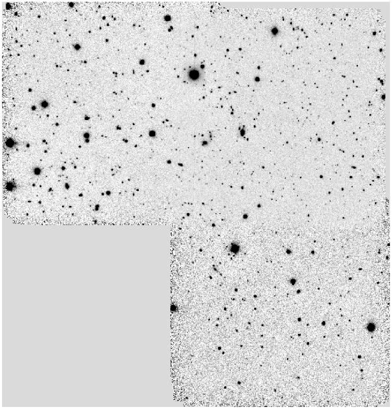
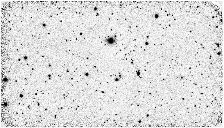
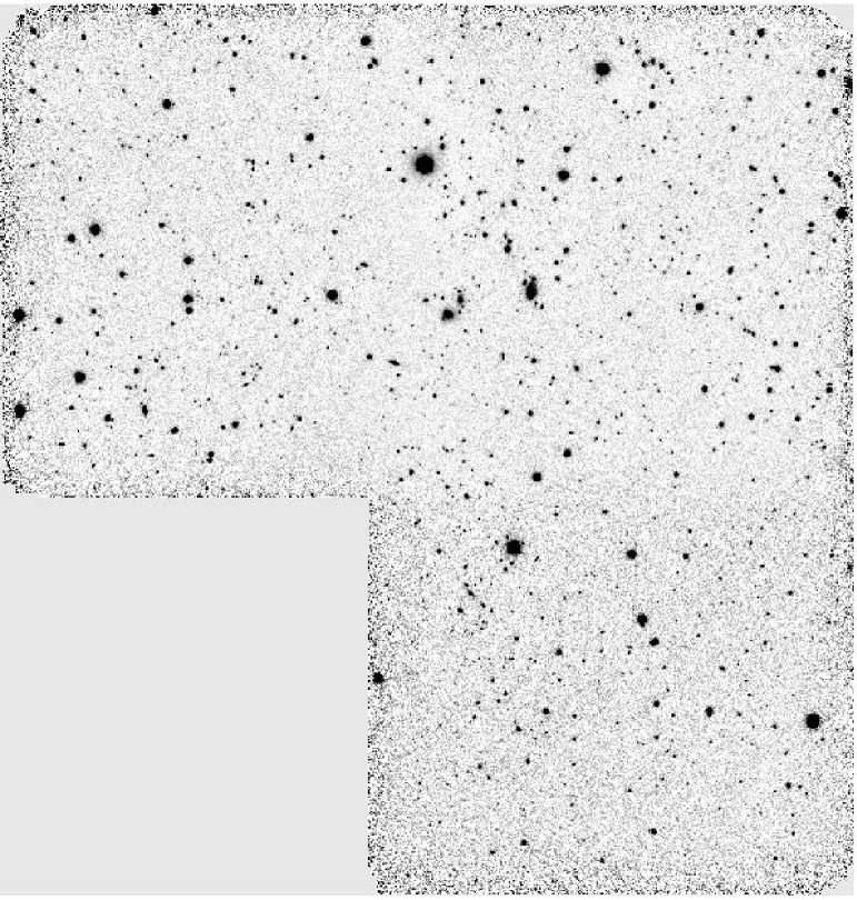
Figure 1: Mosaic image of the HDF-S in the $J$, $H$ and $K_{s}$-band from top to bottom.

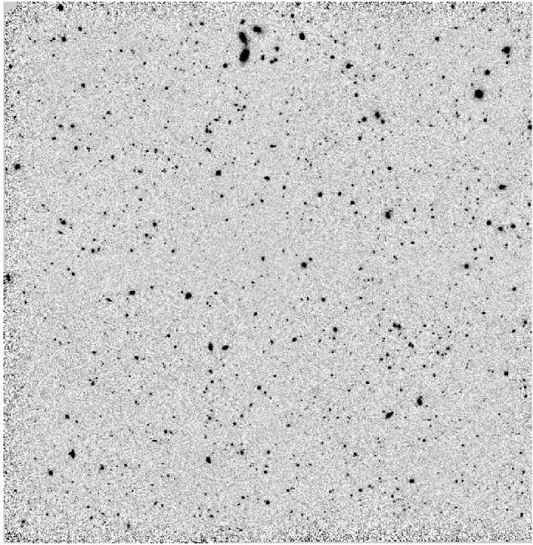
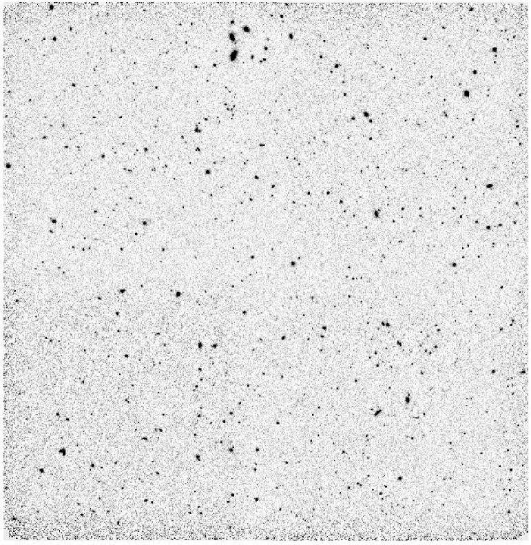
Figure 2: Mosaic image of the CDF-S in the $J$ (upper) and $K_{s}$-band (lower).

4.1 Images

The 62 reduced images mentioned in the previous section were converted into 17 stacked (co-added) images following the procedures described in Paper I. All stacked images were visually inspected and graded. Again the quality was found to be good with 14 images being graded A and the remaining 3 B. The resulting mosaics in each passband are shown in Figs. 1 and 2 for HDF-S and CDF-S, respectively.

Table 8: Main characteristics of the final stacks.

Field	Passband	Grade	PSF FWHM	PSF rms	$m_{lim}$ (Vega)	Completeness
CDF-S-1	$J$	A	0.84	0.194	22.72	94%
CDF-S-1	$K_{s}$	A	0.97	0.183	21.08	105%
CDF-S-2	$J$	A	0.92	0.139	22.86	89%
CDF-S-2	$K_{s}$	A	0.70	0.189	20.90	90%
CDF-S-3	$J$	A	0.80	0.194	22.95	99%
CDF-S-3	$K_{s}$	B	1.12	0.123	20.75	84%
CDF-S-4	$J$	A	0.64	0.111	21.44	89%
CDF-S-4	$H$	A	0.84	0.113	21.21	32%
CDF-S-4	$K_{s}$	A	0.87	0.122	20.64	49%
HDF-S-1	$J$	A	1.22	0.113	22.79	156%
HDF-S-1	$H$	B	0.77	0.187	21.47	103%
HDF-S-1	$K_{s}$	A	0.82	0.212	21.34	208%
HDF-S-2	$J$	A	0.83	0.159	21.98	88%
HDF-S-2	$H$	A	0.84	0.181	21.69	112%
HDF-S-2	$K_{s}$	A	1.08	0.176	21.20	198%
HDF-S-3	$J$	A	1.17	0.060	22.07	33%
HDF-S-3	$K_{s}$	B	0.79	0.127	20.80	67%

The main attributes of the stacks produced for each mosaic are summarized in Table 8. The table gives in Col. 1 the field name; in Col. 2 the passband; in Col. 3 the grade; in Cols. 4 and 5 the point-spread function (PSF) FWHM in arcseconds and its anisotropy (PSF rms) as measured in the final stacked image; in Col. 6 the limiting magnitude, $m_{lim}$, estimated for the final image stack for a 2″aperture, $5\sigma$ detection limit in the Vega system; in Col. 7 the completeness of the observations expressed as the fraction (in percentage) of observing time relative to that originally planned. It can be seen that the seeing is, in general, quite good, ranging from 0.64 to 1.22 arcsec with a median of 0.84 arcsec. The median limiting magnitudes in the Vega system are 22.72, 21.47 and 20.90 in the $J$, $H$, and $K_{s}$-band, corresponding to 23.62, 22.84 and 22.74 in the AB-system.

As a final check of the quality of the photometric calibration, the regions of overlap between adjacent frames were used to estimate the relative field-to-field magnitude variations, yielding an estimate of the overall uncertainty in the absolute calibration. In the HDF-S there are only two overlaps in $J$  and $K_{s}$, with the mean values being 0.05 and 0.07, and comparable scatter. In the $H$-band there is only one overlap with an offset of 0.05. For the CDF-S there are four overlaps for the $J$  and $K_{s}$ data, yielding a mean offset of 0.03 and 0.02 mag and a scatter of 0.029 and 0.024 mag, respectively. From these results one can estimate the accuracy of the absolute calibration of HDF-S is $\sim$ 0.05 mag, while that of CDF-S is considerably better $\lesssim 0.03$ mag in both bands.

4.2 Catalogs

Table 9: Main characteristics of the catalogs extracted from the final images.

Field	Passband	Eff. area	# Objects	$m_{lim}$ (Vega)
CDF-S-1	$J$	26.3	448	21.56
CDF-S-1	$K_{s}$	25.9	362	19.56
CDF-S-2	$J$	25.6	453	21.78
CDF-S-2	$K_{s}$	25.2	320	19.67
CDF-S-3	$J$	26.3	459	21.45
CDF-S-3	$K_{s}$	26.3	352	19.76
CDF-S-4	$J$	25.9	431	21.68
CDF-S-4	$H$	25.9	227	19.95
CDF-S-4	$K_{s}$	25.9	230	19.13
HDF-S-1	$J$	25.9	460	21.59
HDF-S-1	$H$	25.9	442	19.64
HDF-S-1	$K_{s}$	25.9	496	19.30
HDF-S-2	$J$	26.3	672	21.87
HDF-S-2	$H$	25.6	564	19.81
HDF-S-2	$K_{s}$	26.3	521	20.10
HDF-S-3	$J$	25.2	262	20.81
HDF-S-3	$K_{s}$	26.3	395	19.34

Catalogs were extracted from the stacked images using the EIS Data Reduction System adopting the same procedure as described in Paper I, which also describes the catalog format. The final science-grade catalogs presented include only objects with $S/N\geq 5$ as computed from the magnitude error. Table 9 summarizes the characteristics of the extracted catalogs. The table gives in Col. 1 the field name; in Col. 2 the passband; in Col. 3 the effective area in square arcmin; in Col. 4 the number of objects; and in Col. 5 the 80% completeness limit in the Vega system, $m_{lim}$, as estimated from mock catalogs.

Each catalog and its associated product log, including extensive comparison with other data previously ingested in the associated database of the EIS system, takes about 2.5 min, corresponding to an overall mean data rate of 0.03 Mpix/s.

5 Discussion

The EIS-DEEP infrared data presented here was used as the test case for the implementation of both the stand-alone version of the image processing library EIS/MVM, and the EIS Data Reduction System as a whole. The latter is responsible for a variety of automatic and un-supervised processes ranging from the creation of the reduction blocks and of the reduced images on a nightly basis to the creation of stacks and their associated final science-grade catalogs presented in the previous section. Because the EIS-DEEP infrared dataset is at the same time relatively small, enabling extensive tests to be done, and large enough to sample a variety of problems that emerge under real observing conditions, thereby helping identify trouble-spots in the code, it provides an excellent test case. Furthermore, this dataset has been reduced both by the EIS team, using different software packages (da Costa et al., 1998; Rengelink et al., 1998) or versions of the same software (Vandame et al., 2001, and the present paper), and independently by other groups using different techniques, thereby allowing the comparison of different versions. Finally, several other datasets covering the regions considered have been compiled since the completion of the EIS-DEEP observations, using either the same or different instruments with different limiting magnitudes. The availability of these various datasets discussed below is in marked contrast to the time these data were first released by the EIS team.

The availability of this large array of different datasets covering the same region allows a careful assessment of the performance of the EIS system and the quality of its final science products by direct comparison of the position, flux scale and absolute calibration of objects in common between source catalogs extracted from different final images. Additionally, statistical measures, here limited to number counts of galaxies and stars, compared to those computed by other authors or predicted by models are used to assess the overall consistency with results from the literature.

5.1 Comparison with other reductions

The comparison with other reductions of the same dataset has been extensively used to show, a posteriori, the shortcomings of previous releases of this dataset either produced by the original implementation of the program Jitter of Eclipse (Devillard et al., 1999) or by an earlier version of the new EIS/MVM image processing library. Below, the same strategy is adopted to evaluate the performance of the current version of the system also used in the reduction of the infrared part of the DPS survey to be presented in a forthcoming paper (Olsen et al., 2006) and of the optical data in Dietrich et al. (2005); Mignano et al. (2006).

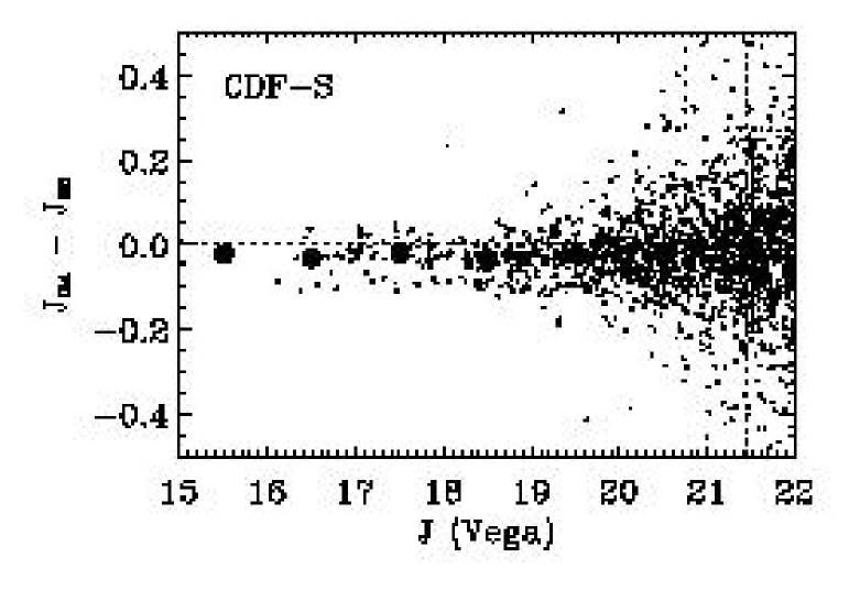
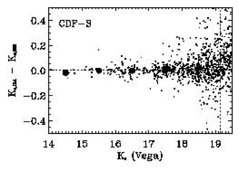
Figure 3: Comparison between the measured $J$ (upper panel), and $K_{s}$ (lower panel) magnitudes of objects in common with those from Vandame et al. (2001). The large filled circles represent the mean magnitude difference computed in bins of 1 mag, while the error bars denote the scatter in each bin. All magnitudes are in the Vega system.

As a starting point, Fig. 3 shows the difference in magnitude of objects identified in images produced using an earlier version of the EIS/MVM library, as reported in Vandame et al. (2001), and those of the most recent version of the package, in all four fields of the CDF-S region. The objects were matched by positional coincidence, using a search radius of 1 arcsec, and only 5$\sigma$ detections are considered. These values are used throughout this paper. The large filled circles are the mean value of the magnitude differences in bins of one magnitude, and the error bars indicate their scatter. The vertical dashed lines in the figure denote the brightest magnitude $m_{lim}$, of the four fields considered, where $m_{lim}$ is the magnitude at which the completeness of the catalog drops to 80%. From the top panel one finds that the error in the earlier version of the image processing library had little effect in the relative photometry of the $J$-band data, with the possible exception of the faintest magnitude bin, which shows the hallmark of lost flux in the older reduction. Surprisingly, after re-calibration one also finds that the $J$ magnitudes for one of the fields exhibits an offset with respect to the others of as much as 0.1 mag. Closer inspection of the data shows that this is associated to the field CDF-S-4. From the bottom panel, one finds that in the $K_{s}$-band the effects of flux loss are slightly larger but still of the order of $\lesssim$ 0.05 mag, significantly smaller than the originally reported bias, which reached 0.15 mag at the faint end.

Figure 4: Difference in magnitudes $J$ (top panels) and $K_{s}$ (lower panels) as measured reducing the infrared data using the DIMSUM package (Daddi private communication) and the EIS software. As before, the large filled circles are the mean values of the difference in bins of one magnitude and the error bars are the scatter.

To further verify the quality of the produced stacks, the $J$- and $K_{s}$-band images of the CDF-S fields 1 and 2 reduced using the IRAF package DIMSUM (Daddi, private communication) were used to extract catalogs, in the same way as those created by the EIS system. The catalogs were matched and the magnitudes of the objects in common compared. In this comparison, the absolute calibration has been neglected and any residual offset at the bright end between the two sets of catalogs was arbitrarily removed. The results are shown in Fig. 4 with the top panels showing the results for the $J$-band and the bottom panels for the $K_{s}$-band, for the fields indicated in each panel. As can be seen from the comparison in both bands and fields the results are excellent, demonstrating that the earlier problems identified in the image processing system have been properly addressed.

Similar results were obtained comparing other reductions of SOFI and ISAAC data, reduced using either the same or different software (e.g. Saracco, private communication; Dickinson, private communication). In summary, it has been shown that the current reductions of the infrared data obtained using the EIS Data Reduction System is free from any flux bias at faint magnitudes, yielding results in excellent agreement with those obtained using other software packages designed specifically to deal with infrared data.

5.2 Comparison with other datasets

Figure 5: Position (left panels) and magnitude (right panels) differences (2MASS-EIS) between EIS sources in common with those identified by the 2MASS survey (Kleinmann et al., 1994) showing the results in different passbands with $J$  on top and $K_{s}$ on the bottom.

Figure 6: Magnitude difference (FIRES-EIS) between EIS sources in common with FIRES (Labbé et al., 2003) objects, as a function of the EIS magnitude. The filled circles and error bars are defined as in the previous figure. All magnitudes are in the Vega system.

Figure 7: Position (left panel) and magnitude differences (right panel) between EIS sources in common with those identified by Moy et al. (2003) in the CDF-S region, as a function of the EIS magnitude. The filled circles and error bars are defined as in the previous figure. All magnitudes are in the Vega system.

Figure 8: Same as Fig. 7 but now comparing positions and magnitudes measured by the LCIRS of the HDF-S.

The validation of the infrared reductions presented here can be extended, comparing them to other fully calibrated datasets available in the literature and covering the same regions surveyed by EIS-DEEP. Examples of these datasets include: 1) data from the Two Mass All Sky Survey (2MASS, Kleinmann et al., 1994) in all three passbands, useful to check the bright end; 2) deep data taken with ISAAC at the VLT for the FIRES survey (Labbé et al., 2003) covering one of the pointings of the HDF-S region; 3) data taken in H-band of the CDF-S region by Moy et al. (2003); and data from the Las Campanas Infrared Survey (LCIRS, Chen et al., 2002) of the HDF-S region.

The results of these various comparisons are shown in Figs. 5–8. Fig. 5 shows the offset in position (left panels) and magnitude (right panels) for objects in common with 2MASS within 1 arcsec of EIS-DEEP detections. Each row shows the results obtained combining all the fields for the different bands with $J$ on top and $K_{s}$ on the bottom. While the number of objects is relatively small, considering the magnitude interval of the two samples, the main advantage of 2MASS is that data are available for all fields allowing the use of a single reference to check both the astrometric and photometric calibration. From Fig. 5 one finds that there is a relative offset between the reference system of the two datasets. However, this offset is nearly the same for all passbands ranging from 0.27 to 0.43 arcsec in right ascension and from 0.19 to 0.26 arcsec in declination with a scatter of $\lesssim 0.40$ arcsec in all bands. Since the objects in common are predominantly from HDF-S, the observed offset reflects the difference between the Tycho and GSC2 coordinates in the HDF-S region. As shown by (Olsen et al., 2006), no systematic shifts are found relative to the USNO-B catalog used to calibrate the different regions covered by the DPS infrared dataset.

Comparison of the magnitudes yields offsets of -0.02, 0.004, and -0.05 mag in $J$, $H$ and $K_{s}$, respectively, if one discards very bright objects which tend to be partly saturated in the deep data. Another important fact is that, except for the Malmquist bias seen in the plots, there is no evidence of systematic trends with magnitude in the interval considered. Furthermore, the small scatter suggests some degree of consistency between the calibration of the images involving as much as 7 fields distributed over two distant regions of the sky, in some cases observed in different nights. All this evidence suggests a consistent absolute calibration of the EIS-DEEP data.

The behavior at faint magnitudes is evaluated by comparing the present data to the deep observations of the FIRES survey (Labbé et al., 2003). Since the authors do not provide the data with an astrometric solution a crude shift has been applied to obtain a proper match between the final images derived for the two datasets. Therefore, in this case only magnitudes are compared. Furthermore, in the comparison only objects detected at 5$\sigma$ in both catalogs are considered. Fig. 6 shows the result of this comparison for all the available passbands. From the figure one finds that regardless of the passband, there is no systematic deviation of the magnitude differences as a function of the magnitude apart from a constant offset. One possible exception is the difference at the faintest bin in the $J$-band, which seems to reflect the effects of a Malmquist bias rather than flux-loss at the faint end. The comparison yields offsets of -0.11, 0.06 and 0.001 mag in $J$, $H$ and $K_{s}$, respectively.

In the $H$-band two more datasets are available for comparison. One is that of Moy et al. (2003) covering the CDF-S region, for which there is an overlap with the somewhat shallow EIS-DEEP observations of CDF-S-4, and the other is that obtained as part of the LCIRS coverage of the HDF-S region. The results of the comparison with Moy et al. (2003) are shown in Fig. 7, where the differences in position (left panel) and magnitude (right panel) of objects in common are plotted. The mean offset in position is less than 0.1 arcsec with an rms of about 0.45 arcsec, consistent with both having an error of the order of $\sim 0.25$ arcsec. This result shows that the positions in the CDF-S region have no systematic shift. The magnitudes are also in good agreement except for an offset of 0.1 mag, somewhat larger than the 0.06 mag derived from the comparison with FIRES data of HDF-S. The origin of this offset is unknown and may be due to an inadequate absolute calibration. However, this calibration can only be improved by additional observations under photometric conditions and a better calibration plan. Again there is no systematic deviation of the magnitude differences over the entire magnitude interval considered. This is in marked contrast with the results obtained comparing the EIS data with the LCIRS $H$-band data taken in the region of the HDF-S, shown in Fig. 8. Here the magnitude difference tends to increase for fainter objects, with the LCIRS magnitudes being fainter than those assigned by the EIS system. This trend reaches about 0.2 mag relative to the bright end, except for the faintest bin shown affected by the Malmquist bias. Since this effect is not seen in any of the other comparisons discussed above, it suggests that this effect stems from the LCIRS reductions. Note that the offset in the bright end is $0.12\pm 0.07$, consistent with that computed from the comparison with Moy et al. (2003) of 0.1 mag, but somewhat larger than the offset of 0.06 mag measured against FIRES. Still, regardless of the exact value this result also suggests a remarkable consistency in the photometric calibration of the CDF-S and HDF-S regions. On the other hand, the left panel of Fig. 8 shows the same offset in the coordinates as observed relative to the 2MASS data. Note that the absolute differences can easily be corrected. To construct optical/infrared catalogs the astrometric calibration of infrared images should be done using catalogs extracted from the optical images, thereby minimizing possible relative offsets.

5.3 Comparison of galaxy and star counts

It is not always possible to assess the quality of the data by direct comparison with overlapping observations. An alternative is to compute different statistical measures, the simplest examples being galaxy and star counts, and compare them with those obtained by other authors in other regions of the sky, typically used for galaxies, or for stars with those predicted by models of the Galaxy.

Figs. 9 and  10 show the galaxy counts computed from the catalogs extracted from the EIS-DEEP images of each field (columns) and passband (rows) of the HDF-S and CDF-S regions, respectively. This is done in order to minimize differences that could be introduced in mean counts from field-to-field variations in depth of the observations. Here all objects with stellarity index $<$ 0.95 were classified as galaxies. The present counts are compared to those published earlier by different authors (Väisänen et al., 2000; Martini, 2001; Iovino et al., 2005). The good agreement between the various counts is further evidence of the scientific quality of the data and calibration presented in this paper. One can also see the strong field-to-field variations in limiting magnitude, a problem one must take into account when dealing with mosaics covering large areas of the sky.

For completeness, Figs.  11 and  12 show similar plots for the stellar counts, comparing them with the predictions of the Galactic model of Girardi et al. (2005). Considering the uncertainties involved in the model and the shot-noise the agreement is quite remarkable, with the possible exception of the $K_{s}$ counts in the CDF-S-1 and -3.

Figure 9: Galaxy number counts computed from the present data for each band (rows) and field (columns) of the HDF-S region (solid circles) compared to the published values with diamonds denoting those of Väisänen et al. (2000); triangles Martini (2001) and squares Iovino et al. (2005) .

Figure 10: Same as Fig. 9 but for the CDF-S region.

Figure 11: Star counts in the three passbands (rows) for the three fields (columns) covering HDF-S (full circles) compared to the predictions (solid line) computed from the model of Girardi et al. (2005).

Figure 12: Same as Fig. 11 but for the four fields of CDF-S

6 Summary

This paper presents the results of the infrared part of the EIS-DEEP survey carried out in the period 1998-1999 covering the HDF-S and CDF-S regions. The paper includes re-processed and re-calibrated images of previously released data, as well as new sets of data not released before. These data are available at the CDS and supersede earlier releases described in the preprints by da Costa et al. (1998); Rengelink et al. (1998) and Vandame et al. (2001) which represent different phases of the project. In contrast to the original release, new datasets have become available, allowing a critical examination of the results by carrying out an array of direct comparisons with reductions of the same dataset as well as comparison with independent datasets.

The results show that the past problems with flux loss of Jitter and an earlier version of the EIS/MVM library have been successfully corrected with the magnitudes measured from the EIS images showing no systematic deviations relative to those derived from images reduced using other reduction techniques. Furthermore, comparisons with data obtained by other authors also suggest that the absolute calibration is reliable to within $\sim 5-10\%$. To obtain a better accuracy would require additional observations under photometric conditions and a good sampling of standards over the entire night.

The results obtained in this paper, combined with those discussed in previous papers of this series, demonstrate the power and versatility of the EIS Data Reduction System which can be used to efficiently process optical and infrared data in the same environment yielding reliable results. The EIS-DEEP survey was the precursor of the the Deep Public Survey (DPS), which combines optical wide-field imaging with infrared data. The results of this survey will be reported in forthcoming papers of this series (Olsen et al., 2006; Mignano et al., 2006). Combined, these data provide information in up to seven bands from the ultraviolet to the near-infrared, thus being an excellent test case for future optical/infrared surveys. The results presented here and in other papers of this series demonstrate that the EIS Data Reduction System meets the requirements for long-term programs using the VST and VISTA survey telescopes.