[
Long range correlation in cosmic microwave background radiation
Abstract
We investigate the statistical anisotropy and Gaussianity of temperature
fluctuations of Cosmic Microwave Background radiation (CMB) data
from Wilkinson Microwave Anisotropy Probe survey, using the
multifractal detrended fluctuation analysis, rescaled range and
scaled windowed variance methods. The multifractal detrended
fluctuation analysis shows that CMB fluctuations has a long range
correlation function with a multifractal behavior. By comparing the
shuffled and surrogate series of CMB data, we conclude that the
multifractality nature of temperature fluctuation of CMB is mainly
due to the long-range correlations and the map is
consistent with a Gaussian distribution.
PACS numbers: 05.10.-a ,05.10.Gg, 05.40.-a, 98.80.Es, 98.70.Vc
]
I Introduction
The Wilkinson Microwave Anisotropy Probe (WMAP) mission is designed to determine the geometry, matter content, and the evolution of the universe. It is shown that the universe is geometrically flat and dark energy at the present time has the dominant contribution in the matter content of the universe, causes the universe to have positive acceleration [1, 2, 3, 4]. The statistical properties of the Cosmic Microwave Background radiation (CMB) data can be a unique tool to identify the parameters of standard model of cosmology [5]. One of the main aims of the statistical analysis of the CMB is to examine the early universe scenarios as the inflationary cosmology. The Gaussianity of primordial fluctuations is a key assumption of modern cosmology, motivated by inflationary models [6, 7, 8].
Since the observed CMB sky is a single realization of the map of the large scale structures, the detection of statistical isotropy violation or correlation patterns pose a great observational challenge. In order to extract more information from the rich source of information provided by present (and future) CMB maps [9, 10, 11], it is important to design as many independent statistical methods as possible to study deviations from standard statistics, such as statistical isotropy and possible correlations. Since statistical isotropy can be violated in many different ways [12], various statistical methods can come to different conclusions. Each method by design is more sensitive to a special kind of statistical isotropy violation [13, 14, 15]. Based on bipolar power spectrum, it has shown no strong evidence of statistical isotropy violation [16, 17, 18], but analysis of the distribution of extrema in WMAP sky maps has indicated non-Gaussianity and to some extent, violation of statistical isotropy [19]. In addition there are many criteria have been introduced to measure the statistical isotropy of CMB such as, quadratic maximum-likelihood [20], multipole vectors [21] and more recently P. Naselsky et. al. used symmetry of CMB map to determine statistical isotropy as well as non-Gaussianity [22].
The statistical properties of the primordial fluctuations generated by the inflationary cosmology are closely related to the cosmic microwave background radiation anisotropy and a measurement of non-Gaussianity is a direct test of the inflation paradigm (see Refs. [23, 24] for more details). Many authors have searched for non-Gaussian signatures in CMB data using peak distributions [25, 26], the genus curve [27, 28], peak correlations [29], global Minkowski functionals methods [30] and directional spherical wavelet [31, 32]. The techniques used for the detection of non-Gaussianity in hydrodynamic turbulence was applied for CMB data [33, 34]. Moreover the Gaussianity of CMB in different angular scales have been tested [35, 36, 37, 38, 39, 40, 41, 42, 43, 44, 45, 46, 47, 48, 49, 50, 51, 52, 53, 54, 55, 56, 57, 58, 59, 60, 61, 62, 63, 64]. Most of the previous works only tested the consistency between the CMB data and simulated Gaussian realizations and so far they found no significant evidence for cosmological non-Gaussianity.
In this work we characterize the complex behavior of CMB through the computation of the fluctuation parameters - scaling exponents - which quantifies the correlation exponents and multifractality of the data. We use certain fractal analysis approaches such as, Multifractal Detrended Fluctuation Analysis (MF-DFA), Rescaled Range Analysis and Scaled Windowed Variance (SWV) to analysis the data set. Using the new approaches, we will test the statistical isotropy and Gaussianity of temperature fluctuations at the last scattering surface. The MF-DFA method shows that Cosmic Microwave Background fluctuations has a long range correlation function with multifractal behavior. Comparing the MF-DFA results of the original temperature fluctuations to those for shuffled and surrogate series, we conclude that the multifractality nature of CMB is mainly due to long-range correlations and the map is consistent with Gaussian distribution. Applied methods of MF-DFA, and SWV, show that WMAP data is a statistically isotropic data set. The value of scaling exponent (Hurst exponent) guarantees that there is no evidence for violation of statistical isotropy in the CMB anisotropy map considered here.
This paper is organized as follows: In Section II we briefly describe
the MF-DFA method and show that the scaling exponents determined via the
MF-DFA method are identical to those obtained by the standard
multifractal formalism based on partition functions. Also briefly
introduce the Rescaled Range Analysis and Scaled Windowed Variance
methods. The fractal analysis of the temperature fluctuations are
presented in Section III. In Section IV, we compare the multifractal
behavior of the original data with that of shuffled and surrogate
series and show that the multifractality is mainly due to the
long-range correlations. In Section V we investigate the statistical
isotropy and Gaussianity of temperature fluctuations using the
MF-DFA, R/S and SWV results. Section VI provides
discussion and presents the results.
II Fractal Analysis Methods
In this section we review three standard methods, i.e. MF-DFA, and SWV, to investigate the fractal properties of stochastic processes.
A Multifractal Detrended Fluctuation Analysis
The MF-DFA methods are the modified version of detrended fluctuation analysis (DFA) to detect multifractal properties of series. The detrended fluctuation analysis (DFA) method introduced by Peng et al. [65] has became a widely-used technique for determination of (mono)-fractal scaling properties and the detection of long-range correlations in noisy non-stationary time series [65, 66, 67, 68, 69]. It has successfully been applied to diverse fields such as DNA sequences [65, 70], heart rate dynamics [71, 72], neuron spiking [73], human gait [74], long-time weather records [75], cloud structure [76], geology [77], ethnology [78], economical time series [79], solid state physics [80], solar physics and plasma fluctuations [81].
The simplest type of the multifractal analysis is based upon the standard partition function multifractal formalism, which has been developed for the multifractal characterization of normalized, isotropic (stationary) measurements [82, 83, 84, 85]. Unfortunately, this standard formalism does not give correct results for non-isotropic angular (non-stationary time) series that are affected by trends or that cannot be normalized. Thus, in the early 1990s an improved multifractal formalism has been developed, the wavelet transform modulus maxima (WTMM) method [86], which is based on the wavelet analysis and involves tracing the maxima lines in the continuous wavelet transform over all scales. The other method, the multifractal detrended fluctuation analysis (MF-DFA), is based on the identification of scaling of the th-order moments depending on the signal length and is a generalization of the standard DFA using only the second moment .
The MF-DFA does not require the modulus maxima procedure in contrast to the WTMM method, and hence does not require more effort in programming and computing than the conventional DFA. On the other hand, often experimental data are affected by non-isotropic (non-stationarities) like trends, which have to be well distinguished from the intrinsic fluctuations of the system in order to find the correct scaling behavior of the fluctuations. In addition very often we do not know the reasons for underlying trends in collected data and even worse we do not know the scales of the underlying trends, also, usually the available recorded data is small. For the reliable detection of correlations, it is essential to distinguish trends from the intrinsic fluctuations in the data. Non-detrending methods work well if the records are long and do not involve trends. But if trends are present in the data, they might give wrong results. Detrended fluctuation analysis (DFA) is a well-established method for determining the scaling behavior of noisy data in the presence of trends without knowing their origin and shape [65, 70, 71, 87, 88]
The modified multifractal DFA (MF-DFA) procedure consists of five steps. The first three steps are essentially identical to the conventional DFA procedure (see e. g. [65, 66, 67, 68, 69]). In our case which is studying the temperature fluctuations of CMB, we take the temperature data with the size of and follow the steps as follows:
Step 1: Determine the “profile”
| (1) |
where is the temperature of CMB map, is the unit vector pointing CMB and is the size of segment of CMB that we are calculating the series. Subtraction of the mean is not compulsory, since it would be eliminated by the later detrending in the third step.
Step 2: Divide the profile into non-overlapping segments of equal angular lengths .
Step 3: Calculate the local trend for each of the segments by fitting a polynomial function to . The variance between and the function of the best fit for each segment , , is as follows:
| (2) |
A Linear, quadratic, cubic, or higher order polynomials can be used in the fitting procedure (conventionally called DFA1, DFA2, DFA3, ) [65, 67, 68, 72].
Step 4: Average over all segments to obtain the -th order fluctuation function, defined as:
| (3) |
where, in general, the index variable can take any real value except zero. For , equation (3) becomes:
| (4) |
For , the standard DFA is retrieved. Generally we are interested in how the generalized dependent fluctuation functions, , depend on the angular scale for different values of . Hence, we must repeat steps 2, 3 and 4 for several angular scales . It is apparent that will increase with the increasing of .
Step 5: Determine the scaling behavior of the fluctuation functions by analyzing log-log plots of versus for each value of . If the series are long-range power-law correlated, increases, for large values of , as a power-law
| (5) |
In general, the exponent may depend on . For isotropic fluctuations, and is identical to the well-known Hurst exponent [65, 66, 82]. In the absence of statistical isotropy the corresponding scaling exponent of is larger than unity and its relation to the Hurst exponent is [65, 81, 89]. Thus, one can call the function as the generalized Hurst exponent.
For monofractal fluctuations, is independent of , since the scaling behavior of the variances is identical for all segments of , and the averaging procedure in Eq. (3) will just give this identical scaling behavior for all values of . If we consider positive values of , the segments with large variance (i. e. large deviations from the corresponding fit) will dominate the average . Thus, for positive values of , describes the scaling behavior of the segments with large fluctuations. Usually the large fluctuations are characterized by a smaller scaling exponent for multifractal series [90]. On the contrary, for negative values of , the segments with small variance will dominate the average . Hence, for negative values of , describes the scaling behavior of the segments with small fluctuations [90].
1 Relation to standard multifractal analysis
For an isotropic series the multifractal scaling exponents defined in Eq. (5) are directly related to the scaling exponents defined by the standard partition function-based multifractal formalism as shown below. Suppose that the data of length is an isotropic sequence. Then the detrending procedure in step 3 of the MF-DFA method is not required, since no trend has to be eliminated. Thus, the DFA can be replaced by the standard Fluctuation Analysis (FA) with the definition of variance for each segment , as follows:
| (6) |
| (7) |
In order to relate also to the standard textbook box counting formalism [82, 83, 84, 85], we employ the definition of the profile in Eq. (1). It is evident that the term in Eq. (7) is identical to the sum of the numbers within each segment of size . This sum is known as the box probability in the standard multifractal formalism for :
| (8) |
The scaling exponent is usually defined via the partition function
| (9) |
where is a real parameter as in the MF-DFA method, discussed above. Using Eq. (8), we see that Eq. (9) is identical to Eq. (7), and obtain analytically the relation between the two sets of multifractal scaling exponents
| (10) |
Thus, we observe that defined in Eq. (5) for the MF-DFA is directly related to the classical multifractal scaling exponents . Note that is different from the generalized multifractal dimensions which is defined as:
| (11) |
that are used instead of in some papers. While is independent of for a monofractal time series, depends on in this case. Another way to characterize a multifractal series is the singularity spectrum , that is related to via a Legendre transform [82, 84]
| (12) |
here, is the singularity strength or Hölder exponent, while denotes the dimension of the subset of the series that is characterized by . Using Eq. (10), we can directly relate and to
| (13) |
A Hölder exponent denotes mono-fractality, while in the multifractal case, the different parts of the structure are characterized by different values of , leading to the existence of the spectrum . The interval of Hlder spectrum for a multifractal process, , can be determined by [91]
| (14) | |||||
| (15) |
B Scaled Windowed Variance Analysis
The Scaled Windowed Variance analysis was developed by Cannon et al. (1997)[89]. The profile of temperature, , is divided into intervals of angular length scale . Then the standard deviation is calculated within each interval using the following relation
| (16) |
The average standard deviation of all angular intervals of length is computed. This computation is repeated over all possible interval lengths. The scaled windowed variance is related to by a power law
| (17) |
C Rescaled Range Analysis
Hurst developed the Rescaled Range analysis, a statistical method to analyze long records of natural phenomena [89, 92]. There are two factors used in this analysis: firstly the range , this is the difference between the minimum and maximum ’accumulated’ values or cumulative sum of of a typical natural phenomenon at discrete time over a time span , and secondly the standard deviation , estimated from the observed values . Hurst found that the ratio is very well described for a large number of natural phenomena by the following empirical relation
| (18) |
where and are time span and Hurst exponent, respectively. For temperature fluctuations on the last scattering surface, and are defined as
| (19) | |||||
| (20) |
where is defined according to Eq. (1). The scaling behavior of the fluctuation function is determined by analyzing log-log plot of versus as
| (21) |
III Fractal Analysis of cosmic microwave background radiation data
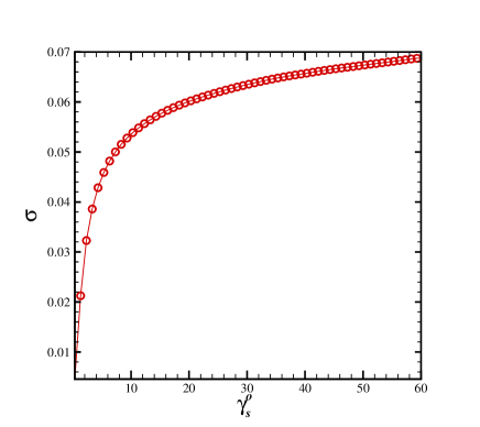
As mentioned in section II, a spurious of correlations may be detected in the absence of statistical isotropy, so direct calculation of correlation functions, fractal dimensions etc., may not give reliable results [65, 66, 82, 89, 90]. The simplest way to verify the statistical isotropy of the temperature fluctuations on the last scattering surface is by measuring the stability of the variance of the temperature in various sizes of windows. Figure 1 shows the standard deviation of the temperature verses the angular size of the window. Here we have a saturation for the standard derivation in the large angular scale which reflects the long-range correlation behavior of the temperature fluctuations of CMB [65, 66, 82, 89, 90].
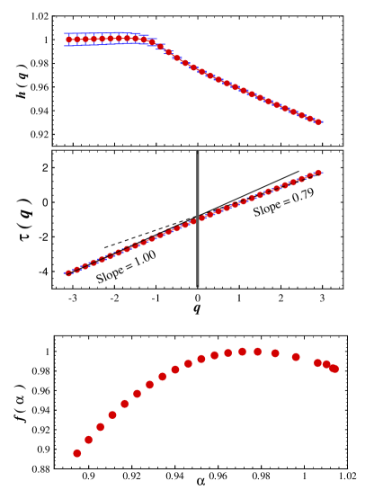
We use the MF-DFA1 method for analyzing the temperature fluctuations on CMB. Following the procedure for MF-DFA analysis as described in the last section we obtain as a function of angular scale . For each index of the generalized Hurst exponents in Eq. (5) can be found by analyzing log-log plots of versus . Figure 2 shows the Hurst exponent in terms of for MF-DFA1 analysis. Variation of Hurst exponent in terms of shows the multifractal behavior of temperature fluctuation of CMB. More over we have different values of the slope of classical multifractal scaling exponent,, for and , which indicates that CMB has a multifractal structure. For positive and negative values of , we obtain with the slopes of and , respectively at confidence interval. According to the relation between the Hurst exponent and MF-DFA exponent, we obtain at confidence interval which means that temperature fluctuation is an isotropic process with long-range correlation [90]. The variation of singularity spectrum , Eq. (12) also is shown in Figure 2. The values of derived quantities from MF-DFA1 method, are given in Table I.
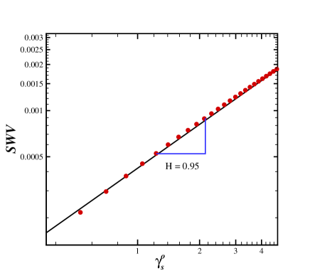
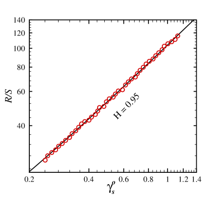
We also use the Scaled Windowed Variance (SWV) analysis [89, 92] to determine the Hurst exponent for CMB via Eq. (17). Figure 3 shows log-log plot of Scaled Windowed Variance of CMB fluctuations as a function of angular scale, which results at confidence interval. Finally we apply the Rescaled Range analysis (), to determine the Hurst exponent of CMB fluctuations. According to Figure 4, the value of Hurst exponent obtain as at confidence interval, which is in agreement with the two previous results.
IV Comparison of multifractal nature for original, shuffled and surrogate CMB data
In this section we are interested in to determine the source of multifractality and test the Gaussianity of CMB data. In general, two different types of multifractality in certain data set can be distinguished: (i) Multifractality due to a fatness of probability density function (PDF) and (ii) Multifractality due to different correlations in small and large scale fluctuations. In the first case the multifractality cannot be removed by shuffling the data set, while in the second case data may have a PDF with finite moments, e. g. a Gaussian distribution and the corresponding shuffled series will exhibit mono-fractal scaling, since all long-range correlations are destroyed by the shuffling procedure.
| Data | |||
|---|---|---|---|
| CMB | |||
| Surrogate | |||
| Shuffled |
If we have both kinds of multifractality in data, the shuffled series will show weaker multifractality than the original series. The easiest way to distinguish the type of multifractality, is by analyzing the corresponding shuffled and surrogate series. The shuffling of data set destroys the long range correlation, therefore if the multifractality only belongs to the long-range correlation, we should find [90]. The multifractality nature due to the fatness of the PDF signals is not affected by the shuffling procedure. On the other hand, to determine the multifractality due to the broadness of PDF by the surrogating method, the phase of discrete fourier transform (DFT) coefficients of CMB data are replaced with a set of pseudo independent uniform distribution within the range of [81, 93]. The correlations in the surrogate series do not change, while the probability function changes to the Gaussian distribution. If multifractality in the data set is due to a broadness of PDF, obtained by the surrogate method will be independent of . If both kinds of multifractality are present in CMB data, the shuffled and surrogate series will show weaker multifractality than the original one.
To check the nature of multifractality, we compare the fluctuation function , for the CMB map with the result of the corresponding shuffled, and surrogated data . Differences between these two fluctuation functions with the original one can indicate the presence of long range correlations or broadness of probability density function in the original data. These differences can be obtained by the ratio and as a function of [90]. Since the anomalous scaling due to a broad probability density affects and in the same way, only multifractality due to correlations will be observed in . The scaling behavior of these ratios are:
| (22) |
| (23) |
If only fatness of the PDF be responsible for the multifractality, one should find and . On the other hand, deviations from indicates the presence of correlations, and dependence of indicates that multifractality is due to the long-rage correlation.
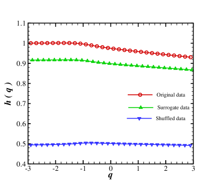
If the multifractal behavior of CMB is made by the broadness of PDF and long-range correlation, both and will depend on . The dependence of the generalized exponent for original, surrogate and shuffled CMB data are shown in Figures 5 which shows that the multifractality nature of temperature fluctuation is almost due to the correlation. The absolute value of is larger than which indicates that the multifractality due to the fatness is much weaker than the multifractality due to the correlation. The deviation of and from can be determined by using as follows:
| (24) |
where the symbol represents for and series. The value of reduced chi-square ( is the number of degree of freedom) for shuffled and surrogate time series are , , respectively.
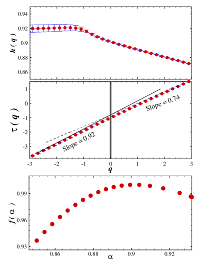
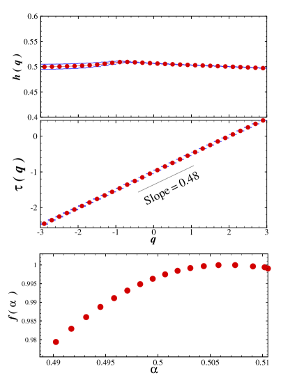
Singularity spectrum of the surrogate series is almost similar to the original temperature fluctuations, while in the case of shuffled series we have a narrower singularity spectrum of compare to that of surrogate and original data . The small value of compare to the two other series shows that the multifractality in the shuffled CMB map has almost been destroyed [94]. Figures 6 and 7 show the MF-DFA1 results for surrogate and shuffled temperature fluctuation series. Comparing the MF-DFA results of the data set to those for shuffled and surrogate series, we conclude that the multifractal nature of temperature fluctuations in CMB data is almost due to the and the probability distribution function of CMB is almost Gaussian (see also the section ). The values of the Hurst exponent , multifractal scaling , generalized multifractal dimension of the original, shuffled and surrogate data of CMB obtained with MF-DFA1 method are reported in Table I.
V Statistical Isotropy and Gaussianity of CMB Anisotropy
In this section we examine the Gaussianity and statistical isotropy of temperature fluctuations in CMB data through MF-DFA, and SWV methods.
Standard models of inflationary cosmology predict a Gaussian distribution of CMB temperature fluctuations. However, along with standard inflationary models, there exist theories such as inflationary scenarios with two or more scalar fields which predict a non-Gaussian primordial fluctuations [95, 96, 97, 98, 99, 100, 101]. Another possibility of deviation from the Gaussianity is the manipulation of the CMB signals after the recombination due to subsequent weak gravitational lensing [102, 103] and various foregrounds like dust emission, synchrotron radiation, or unresolved point sources [104]. One should also take into account the additional instrumental noise in the observational data [105]. One of the advantages of Gaussian field is that the two point correlation function will be sufficient for fully specify the statistical properties of the field. In the case of non-Gaussianity, one must take the higher moments of the field into account in order to fully describe the whole statistics. So, studying the Gaussian nature of the signals or detecting some distinctive non-Gaussianity is an important issue to understand the statistical properties of CMB.
As we have seen in Sec.IV, the MF-DFA1 results of the shuffled series shows almost constant which indicates that is independent of the or in another word the shuffled series is a monofractal structure. This means that the multifractality of the original data is due to the long-range correlations not due to a broadness of PDF of temperature fluctuations (Figure 5). Furthermore small differences in the generalized Hurst exponent between the original and surrogated data (Figure 5) and similarity of the singularity spectrum, , in those two series, show that the probability density function of temperature fluctuations has well confidence with the Gaussian distribution which is in agreement with the recent results [16, 17, 33, 34]
The second important question about the CMB data is its statistical isotropy. One of the main motivations for anisotropy of the universe comes from the global topology of the universe. The idea of a multi-connected topology of the universe comes back to Schwarzschild’s work [106] before the Einstein’s first seminal paper on cosmology [107]. If the universe is assumed to be simply-connected, the cosmological principle implies that it should be globally isotropic to any observer. In the case of multi-connected universe while the Einstein gravity still hold in this space but the global structure of universe at large scales will be more complicated. One of the most promising signatures may be on the CMB as the existence of large scale anisotropies with a repeating patterns [108]. In addition to cosmological mechanisms, instrumental and environmental effects in observations of CMB can also easily produce spurious breakdown of statistical isotropy. Here we examine the anisotropy of CMB with the MF-DFA analysis.
The statistical isotropy means that the statistical properties of CMB (e.g. -point correlations) to be invariant under the Eulerian rotation. This means that two point correlation function is function of angle between two points, i.e.
| (25) |
where is the angle between and . It is then convenient to expand it in terms of Legendre polynomials,
| (26) |
where is the widely used angular power spectrum. The summation over starts from because the term is the monopole which in the case of statistical isotropy the monopole is constant, and it can be subtracted out. The dipole is due to the local motion of the observer with respect to the last scattering surface and can be subtracted out as well. In order to extract the statistical property of CMB we need an ensemble maps from the CMB to calculate the correlation functions. In reality we have only one map from the CMB, but if we assume the statistical isotropy we can calculate the correlation functions moving on overall data. As we mentioned in section II, for a process with stationarity in time or isotropic process in space, the Hurst exponent is always less than unity [65, 89]. According to the MF-DAF1, SWV and methods we obtained the value of Hurst exponent for WMAP data as at confidence interval. These analysis with the Hurst exponent show that there is no evidence for violation of statistical isotropy of WMAP data.
VI Conclusion
In this work we used three method to investigate the statistical properties of WMAP data. The applied methods Multifractal Detrended Fluctuation Analysis, Rescaled Range Analysis and Scaled Windowed Variance methods show that the WMAP data is a statistically isotropic data set. The value of Hurst exponent, , guarantees that there is no evidence for violation of statistical isotropy in the CMB map. The MF-DFA method allows us to determine the multifractal characterization of this map. The dependence of generalized Hurst and classical multifractal scaling exponents, show that the temperature fluctuations on the last scattering surface has multifractal behavior [33]. We obtained the generalized multifractal dimension of CMB data . According to a small difference between generalized Hurst exponent and singularity spectrum of the original data set with the surrogate one’s, and , we found that there is no crucial evidence for non-Gaussianity of the CMB map. The compatibility of the multifractal behavior of the temperature fluctuations of CMB with their Gaussian distribution has been also explored recently [109]. Comparison of the generalized Hurst exponent of the original data with the shuffled and surrogate series showed that the nature of the multifractality of CMB is mainly due to the long-range correlation , rather than the broadness of the probability density function.
Acknowledgements
We would like to thank M. Fazeli and G.R. Jafari for useful discussions.
REFERENCES
- [1] N. Afshordi, Y. Loh, M. A. Strauss, Phys. Rev. D, 69, (2004).
- [2] C. L. Bennett, et al., ApJS, 148, 213 (2003).
- [3] D. N. Spergel, et al., ApJS, 148, 175 (2003).
- [4] M. Tegmark, et al., Phys. Rev. D 69, 103501 (2004).
- [5] H. V. Peiris, et al., ApJS 148, 213 (2003).
- [6] V. F. Mukhanov, G. V. Chibisov, Journal of Experimental and Theoretical Physics Letters, Vol. 33, p.532 (1981).
- [7] S. W. Hawking, Phys. Lett. B 115, 295 (1982).
- [8] A. H. Guth and S. Y. Pi, Phys. Rev. Lett. 49, 1110 (1985).
- [9] Planck Collaboration, arXiv:1101.2028.
- [10] Planck Collaboration, arXiv:1101.2022.
- [11] E. Shirokoff et. al., arXiv:1012.4788.
- [12] L. Ackerman, S.M. Carroll and M.B. Wise, PRD, 75, 083502 (2007).
- [13] Zhen Hou, A.J. Banday, K.M. Gorski, N.E. Groeneboom, H.K. Eriksen, Mon. Not. R. Astron. Soc. 401, 2379-2387 (2010).
- [14] Nidhi Joshi, Sanjay Jhingan, Tarun Souradeep, Amir Hajian, Phys.Rev. D 81, 083012 (2010).
- [15] Moumita Aich, Tarun Souradeep, Phys.Rev. D 81, 083008 (2010).
- [16] Tarun Souradeep and Amir Hajian, astro-ph/0502248.
- [17] Amir Hajian, Tarun Souradeep and Neil Cornish, Ap. J. 618 L63 (2005).
- [18] Amir Hajian and Tarun Souradeep, Phys.Rev. D 74, 123521 (2006).
- [19] D. L. Larson and B. D. Wandelt, Astrophys.J. 613, L85-L88 (2004).
- [20] Duncan Hanson and Antony Lewis, Phys.Rev.D 80, 063004 (2009).
- [21] Caroline Zunckel, Dragan Huterer and Glenn D. Starkman, arXiv:1009.4701.
- [22] P. Naselsky, M. Hansen and J. Kim, arXiv:1105.4426.
- [23] N. Bartolo, S. Matarrese and A. Riotto, Advances in Astronomy, vol. 2010, id. 157079, arXiv:1001.3957.
- [24] L. Raul Abramo and Thiago S. Pereira, Advances in Astronomy, 2010, article id. 378203, arXiv:1002.3173.
- [25] J. M. Bardeen, J. R. Bond, N. Kaiser and A. S. Szalay, Ap. J. 304, 15 (1986).
- [26] J. R. Bond and G. Efstathiou, Mon. Not. Roy. Astron. Soc. 226, 655 (1987).
- [27] P. Coles, Mon. Not. Roy. Astron. Soc. 234, 509 (1988).
- [28] G. F. Smoot, L. Tenorio,A. J. Banday, A. Kogut, E. L. Wright, G. Hinshaw and C. L. Bennett, Ap. J. 437, 1 (1994).
- [29] A. Kogut, A. J. Banday, C. L. Bennett, K. M. Gorski, G. Hinshaw, G. F. Smoot and E. L. Wright, Ap. J. Lett. 464, L29 (1996).
- [30] S. Winitzki, and A. Kosowsky, New Astronomy 3, 75 (1998).
- [31] J. D. McEwen, M. P. Hobson, A. N. Lasenby and D. J. Mortlock, Mon. Not. Roy. Astron. Soc. 388, 659-662 (2008).
- [32] J. D. McEwen, M. P. Hobson, A. N. Lasenby and D. J. Mortlock, Mon. Not. Roy. Astron. Soc. 371 L50-L54 (2006).
- [33] A. Bershadskii and K. R. Sreenivasan, Phys. Lett. A. 319, 21 (2003).
- [34] F. Ghasemi, A. Bahraminasab, M. S Movahed, Sohrab Rahvar, K. R. Sreenivasan and M. Reza Rahimi Tabar, J. Stat. Mech. P11008, (2006).
- [35] A. F. Heavens, Mon. Not. Roy. Astron. Soc. 299, 805 (1998).
- [36] J. A. Peacock and A. F. Heavens, Mon. Not. Roy. Astron. Soc. 217, 805 (1985).
- [37] A. F. Heavens and R. K. Sheth, Mon. Not. Roy. Astron. Soc. 310,1062 (1999).
- [38] A. F. Heavens and Sujata Gupta, Mon. Not. Roy. Astron. Soc. 324, 960 (2001).
- [39] J. Schmalzing and K. M. Gorski, Mon. Not. Roy. Astron. Soc. 297, 355 (1998).
- [40] P. G. Ferreira, J. Magueijo and K. M. Górski, Ap. J. Lett. 503, L1 (1998).
- [41] J. Pando, D. Valls-Gabaud and L. Z. Fang, Phys. Rev. Lett. 81, 4568 (1998).
- [42] B. C. Bromley and M. Tegmark, Ap. J. Lett. 524, L79 (1999).
- [43] A. J. Banday, S. Zaroubi and K. M. Górski, Ap. J. 533, 575 (2000).
- [44] C. R. Contaldi, P. G. Ferreira, J. Magueijo and K. M. Górski, Ap. J. 534, 25 (2000).
- [45] P. Mukherjee, M. P. Hobson and A. N. Lasenby, Mon. Not. Roy. Astron. Soc. 318, 1157 (2000).
- [46] J. Magueijo, Ap. J. Lett. 528, L57 (2000).
- [47] D. Novikov, J. Schmalzing and V. F. Mukhanov, A&A 364, 17 (2000).
- [48] H. B. Sandvik and J. Magueijo, Mon. Not. Roy. Astron. Soc. 325, 463 (2001).
- [49] R. B. Barreiro, M. P. Hobson, A. N. Lasenby, A. J. Banday, K. M. Górski and G. Hinshaw, Mon. Not. Roy. Astron. Soc. 318, 475 (2000).
- [50] N. G. Phillips and A. Kogut, Ap. J. 548, 540 (2001).
- [51] E. Komatsu and U. Seljak, Mon. Not. Roy. Astron. Soc. 336, 1256 (2002).
- [52] E. Komatsu and D. N. Spergel, Phys. Rev. D 63, 63002 (2001).
- [53] M. Kunz, A. J. Banday, P. G. Castro, P. G. Ferreira and K. M. Górski, Ap. J. Lett. 563, L99 (2001).
- [54] N. Aghanim, O. Forni and F. R. Bouchet, A&A 365, 341 (2001).
- [55] L. Cayón, E. Martinez-Gonzalez, F. Argueso, A. J. Banday and K. M. Górski, Mon. Not. Roy. Astron. Soc., 339, 1189 (2003).
- [56] C. Park, B. Ratra and M. Tegmark, Ap. J. 556, 582 (2001).
- [57] S. F. Shandarin, H. A. Feldman, Y. Xu and M. Tegmark, Ap. J. S. 141, 1 (2002).
- [58] J. H. Wu et al., Phys. Rev. Lett. 87, 251303 (2001).
- [59] M. G. Santos, A. Cooray, Z. Haiman, L. Knox and Ch. Ma., Ap. J. 598, 756 (2003).
- [60] G. Polenta et al., Ap. J. Lett. 572, L27 (2002).
- [61] J. M. G. Mead., A. Lewis and L. King, Phys. Rev. D 83, 023507 (2011).
- [62] Bartosz Lew, JCAP 0808:017,2008.
- [63] C. Raeth, G. Rossmanith, G. Morfill, A. J. Banday and K. M. Gorski, arXiv:1005.2481.
- [64] Dragan Huterer, Eiichiro Komatsu and Sarah Shandera, arXiv:1012.3744.
- [65] C. K. Peng, S. V. Buldyrev, S. Havlin, M. Simons, H. E. Stanley and A. L. Goldberger, Phys. Rev. E 49, 1685 (1994); S. M. Ossadnik, S. B. Buldyrev, A. L. Goldberger, S. Havlin, R.N. Mantegna, C.-K. Peng, M. Simons and H.E. Stanley, Biophys. J. 67, 64 (1994).
- [66] M. S. Taqqu, V. Teverovsky and W. Willinger, Fractals 3, 785 (1995).
- [67] J. W. Kantelhardt, E. Koscielny-Bunde, H. H. A. Rego, S. Havlin and A. Bunde, Physica A 295, 441 (2001).
- [68] K. Hu, P. Ch. Ivanov, Z. Chen, P. Carpena and H. E. Stanley, Phys. Rev. E 64, 011114 (2001).
- [69] Z. Chen, P. Ch. Ivanov, K. Hu and H. E. Stanley, Phys. Rev. E 65, (2002).
- [70] S. V. Buldyrev, A. L. Goldberger, S. Havlin, R. N. Mantegna, M. E. Matsa, C. K. Peng, M. Simons and H. E. Stanley, Phys. Rev. E 51, 5084 (1995); S. V. Buldyrev, N. V. Dokholyan, A. L. Goldberger, S. Havlin, C. K. Peng, H. E. Stanley and G. M. Viswanathan, Physica A 249, 430 (1998).
- [71] C. K. Peng, S. Havlin, H. E. Stanley, and A. L. Goldberger, Chaos 5, 82 (1995); P. Ch. Ivanov, A. Bunde, L. A. N. Amaral, S. Havlin, J. Fritsch-Yelle, R. M. Baevsky, H. E. Stanley, and A. L. Goldberger, Europhys. Lett. 48, 594 (1999); Y. Ashkenazy, M. Lewkowicz, J. Levitan, S. Havlin, K. Saermark, H. Moelgaard, P. E. B. Thomsen, M. Moller, U. Hintze and H. V. Huikuri, Europhys. Lett. 53, 709 (2001); Y. Ashkenazy, P. Ch. Ivanov, S. Havlin, C. K. Peng, A. L. Goldberger and H. E. Stanley, Phys. Rev. Lett. 86, 1900 (2001).
- [72] A. Bunde, S. Havlin, J. W. Kantelhardt, T. Penzel, J.-H. Peter and K. Voigt, Phys. Rev. Lett. 85, 3736 (2000).
- [73] S. Blesic, S. Milosevic, D. Stratimirovic and M. Ljubisavljevic, Physica A 268, 275 (1999); S. Bahar, J. W. Kantelhardt, A. Neiman, H. H. A. Rego, D. F. Russell, L. Wilkens, A. Bunde, and F. Moss, Europhys. Lett. 56, 454 (2001).
- [74] J. M. Hausdorff, S. L. Mitchell, R. Firtion, C. K. Peng, M. E. Cudkowicz, J. Y. Wei and A. L. Goldberger, J. Appl. Physiology 82, 262 (1997).
- [75] E. Koscielny-Bunde, A. Bunde, S. Havlin, H.E. Roman, Y. Goldreich and H. J. Schellnhuber, Phys. Rev. Lett. 81, 729 (1998); K. Ivanova and M. Ausloos, Physica A 274, 349 (1999); P. Talkner and R.O. Weber, Phys. Rev. E 62, 150 (2000); R. G. Kavasseri and R. Nagarajian, IEEE Transactions on Circuits and Systems, 51, 2255 (2004).
- [76] K. Ivanova, M. Ausloos, E. E. Clothiaux and T. P. Ackerman, Europhys. Lett. 52, 40 (2000).
- [77] B. D. Malamud and D. L. Turcotte, J. Stat. Plan. Infer. 80, 173 (1999).
- [78] C. L. Alados and M. A. Huffman, Ethnology 106, 105 (2000).
- [79] R. N. Mantegna and H. E. Stanley, An Introduction to Econophysics (Cambridge University Press, Cambridge, 2000); Y. Liu, P. Gopikrishnan, P. Cizeau, M. Meyer, C. K. Peng, and H. E. Stanley, Phys. Rev. E 60, 1390 (1999); N. Vandewalle, M. Ausloos, and P. Boveroux, Physica A 269, 170 (1999); P. Oswiecimka, J. Kwapien and S. Drozdz, Physica A, 347, 626 (2005).
- [80] J. W. Kantelhardt, R. Berkovits, S. Havlin, and A. Bunde, Physica A 266, 461 (1999); N. Vandewalle, M. Ausloos, M. Houssa, P. W. Mertens and M. M. Heyns, Appl. Phys. Lett. 74, 1579 (1999).
- [81] M. Sadegh Movahed, G. R. Jafari, F. Ghasemi, Sohrab Rahvar and M. Reza Rahimi Tabar, J. Stat. Mech. P02003 (2006); S. Kimiagar, M. S. Movahed, S. Khorram, S. Sobhanian and M. Reza Rahimi Tabar, J. Stat. Mech. P03020 (2009).
- [82] J. Feder, Fractals (Plenum Press, New York, 1988).
- [83] A. L. Barabási and T. Vicsek, Phys. Rev. A 44, 2730 (1991).
- [84] H. O. Peitgen, H. Jürgens and D. Saupe, Chaos and Fractals (Springer-Verlag, New York, 1992), Appendix B.
- [85] E. Bacry, J. Delour and J. F. Muzy, Phys. Rev. E 64, 026103 (2001).
- [86] J. F. Muzy, E. Bacry and A. Arneodo, Phys. Rev. Lett. 67, 3515 (1991).
- [87] U. Fano, Phys. Rev. 72, 26 (1947).
- [88] J. A. Barmes and D. W. Allan, Proc. IEEE 54, 176 (1996).
- [89] A. Eke, P. Herman, L. Kocsis and L. R. Kozak, Physiol. Meas. 23, R1-R38 (2002).
- [90] J. W. Gantelhardt, S. A. Zschiegner, E. Kosciliny-Bunde, A. Bunde, S. Pavlin and H. E. Stanley, Physica A 316, 78-114 (2002).
- [91] J. F. Muzy, E. Bacry, and A. Arne’odo, Int. J. of Bifurcation and Chaos 4, 245 (1994); A. Arne’odo, E. Bacry and J. F. Muzy, Physica A 213, 232 (1995).
- [92] H. E. Hurst, R. P. Black and Y. M. Simaika Y M,Long-term storage. An experimental study (Constable, London) (1965).
- [93] D. Prichard and J. Theiler , Phys. Rev. Lett. 73, 951 (1994).
- [94] P. Oświȩcimka et. al., Phys.Rev.E 74, 016103 (2006).
- [95] A. Linde and V. F. Mukhanov, Phys. Rev. D 56, 535 (1997).
- [96] I. Antoniadis, P. O. Mazur and E. Mottola, Comment on ” Nongaussian Isocurvature Perturbations from Inflation’, astro-ph/9705200.
- [97] P. J. E. Peebles, Ap.J. 510, 531 (1999).
- [98] P. J. E. Peebles, Ap.J. 510, 523 (1999).
- [99] M. Sadegh Movahed and Shahram Khosravi, JCAP 1103:012,2011
- [100] J. L. Starck, N. Aghanim and O. Forni, Astron.Astrophys. 416, 9-17 (2004).
- [101] H. Firouzjahi and S.H.H. Tye, JCAP 03 (2005) 009.
- [102] T. Fukushige, J. Makino, O. Nishimura and T. Ebisuzaki, Publications of the Astronomical Society of Japan 47, 493 (1995).
- [103] F. Bernardeau, Astron. Astrophys. 324, 15 (1997).
- [104] A. J. Banday, M. GórskiK, C. L. Bennett, G. Hinshaw, A. Kogut and G. F. Smoot, Ap. J. 468, L85 (1996).
- [105] M. Tegmark, Ap. J. 480, L87 (1997).
- [106] K. Schwarzschild, Vierteljahrsschrift der Astron. Gesellschaft 35, 337 (1900).
- [107] A. Einstein, Sitzungsber. Preu. Akad. Wiss. 142, (1917).
- [108] L. Perivolaropoulos, Phys. Rev. D 48, 1530 (1993).
- [109] A. Bershadskii, Phys. Lett. A360 (2006) 210.