Systematics in the X-ray Cluster Mass Estimators

Abstract

We examine the systematics affecting the X-ray mass estimators applied to a set of five galaxy clusters resolved at high resolution in hydrodynamic simulations, including cooling, star formation and feedback processes. These simulated objects are processed through the X-ray Map Simulator, X-MAS , to provide Chandra -like long exposures that are analyzed to reconstruct the gas temperature, density, and mass profiles used as input. These clusters have different dynamic state: we consider an hot cluster with temperature $T=11.4$ keV, a perturbed cluster with $T=3.9$ keV, a merging object with $T=3.6$ keV, and two relaxed systems with $T=3.3$ keV and $T=2.7$ keV, respectively. These systems are located at $z=0.175$ so that their emission fits within the Chandra ACIS-S3 chip between 0.6 and 1.2 $R_{500}$.

We find that the mass profile obtained via a direct application of the hydrostatic equilibrium equation is dependent upon the measured temperature profile. An irregular radial distribution of the temperature values, with associated large errors, induces a significant scatter on the reconstructed mass measurements. At $R_{2500}$, the actual mass is recovered within 1 $\sigma$, although we notice this estimator shows high statistical errors due to high level of Chandra background. Instead, the poorness of the $\beta-$model in describing the gas density profile makes the evaluated masses to be underestimated by $\sim 40$ per cent with respect to the true mass, both with an isothermal and a polytropic temperature profile. We also test ways to recover the mass by adopting an analytic mass model, such as those proposed by Navarro et al. (1997) and Rasia et al. (2004), and fitting the temperature profile expected from the hydrostatic equilibrium equation to the observed one. We conclude that the methods of the hydrostatic equilibrium equation and those of the analytic fits provide a more robust mass estimation than the ones based on the $\beta-$model. In the present work the main limitation for a precise mass reconstruction is to ascribe to the relatively high level of the background chosen to reproduce the Chandra one. After artificially reducing the total background by a factor of 100, we find that the estimated mass significantly underestimates the true mass profiles. This is manly due (i) to the neglected contribution of the gas bulk motions to the total energy budget and (ii) to the bias towards lower values of the X-ray temperature measurements because of the complex thermal structure of the emitting plasma.

1 INTRODUCTION

The gravitating mass in galaxy clusters is the most fundamental quantity to use them as cosmological probes. Measurements of the total cluster masses have been used for the last 70 years (since Zwicky, 1933) to infer the presence of dark matter over Mpc scales and to constrain the cosmological parameters that describe the distribution and growth of the cosmic density fluctuations of $>10^{14}M_{\odot}$ virialized structures (see the reviews by Rosati et al., 2002; Voit, 2005). These structures appear as well defined and easily observable at the X-ray wavelengths, where the emission is mainly dominated by bremsstrahlung processes and is proportional to the square of the plasma density. This observational evidence allows to identify massive relaxed clusters and to study their physical properties through the estimates of the X-ray emitting intra-cluster medium (ICM) density and temperature. Since the sound crossing time in the ICM is sufficiently shorter than the age of the structure, the assumption that the ICM is in hydrostatic equilibrium within the underlying dark matter potential generally holds (Sarazin, 2002). ICM density and temperature are used to determine the radial mass profile via the hydrostatic equation (see, e.g., Cowie et al., 1987), with a further assumption of the spherical symmetry for the sake of simplicity.

In the present work, we investigate the systematics that affect the X-ray mass measurements by using hydrodynamic simulations processed by our X-ray Map Simulator (X-MAS , Gardini et al., 2004) to produce realistic event files and images that are then analyzed in a way identical to what is done with observed clusters systems. Several authors studied the robustness of the hydrostatic equilibrium and the uncertainties related to this mass estimator. General conclusions were that there is a good agreement between X-ray and true masses, in particular in the outer regions, with a standard deviation of approximately 15 per cent (see, e.g., Schindler 1996; Evrard et al. 1996; cfr. also Bartelmann & Steinmetz 1996). Balland & Blanchard (1997) pointed out, however, that the uncertainties on the mass measurement propagated from the weak constraints on the gas temperature profile via the hydrostatic equilibrium equation make any accuracy on the determination of the mass profile very poor. More recently, Rasia et al. (2004) (see also Kay et al., 2004; Borgani et al., 2004) found in a set of hydro-N-body simulations that the ICM is not in a perfect hydrostatic state and, thus, the masses can be underestimated by up to 20 per cent in non-radiative ICM models due to residual gas bulk motions. Kay et al. (2004) conclude that more thermalization (and less significant departures from the true mass estimates) is obtained when cooling and feedback are included and that an isothermal $\beta$–model still provides accurate mass estimates within 20-30 per cent uncertainties. With our approach in which (1) the known input on the matter distribution is properly convolved with the response of real instruments and (2) an observational-like analysis is performed on the output to recover the original input, we extend the previous work limited to the study of the hydrodynamic simulations in order to highlight the systematic effects present both in the assumption of hydrostatic equilibrium and in the observational techniques adopted in recovering the mass estimates.

The paper is organized as follows. We introduce our simulated dataset in Section 2. The outputs produced by combing the hydrodynamic simulations and the X-ray Map Simulator for Chandra data are presented in Section 3 and analyzed to recover the gravitating mass in Section 4. The results are presented in Section 5 and summarized and discussed in Section 6. All the errors quoted are at $1\sigma$ level (68.3 per cent level of confidence for one interesting parameter).

2 THE SAMPLE OF SIMULATED CLUSTERS

The simulated clusters have been taken from two different simulations in order to obtain a sample with a significant range of masses and dynamical states.

The simulations has been carried out with GADGET-2 (Springel, 2005), a new version of the parallel Tree-SPH simulation code GADGET (Springel et al., 2001). It uses an entropy-conserving formulation of SPH (Springel & Hernquist, 2002), and includes radiative cooling, heating by a UV background, and a treatment of star formation and feedback processes. The latter is based on a sub-resolution model for the multi-phase structure of the interstellar medium (Springel & Hernquist, 2003).

The first cluster, $C_{Hot}$, has been extracted from a dark-matter only simulation with a box-size of 479 $h^{-1}$ Mpc (Yoshida et al., 2001). The assumed cosmological model is a standard flat $\Lambda$CDM universe, with $\Omega_{\rm m}=1-\Omega_{\Lambda}=0.3$, $\sigma_{8}=0.9$, $\Omega_{\rm b}h^{2}=0.019$ and $H_{0}=100h$ km s^-1 Mpc^-1 with $h=0.7$. This cluster has been resimulated at higher mass and force resolution. The new initial conditions for this system have been generated by applying the Zoomed Initial Condition (ZIC) technique (Tormen et al., 1997). This method allows one to increase the mass resolution in a suitably chosen high–resolution Lagrangian region surrounding the structure to be re–simulated, and at the same time to correctly describe the large–scale tidal field of the cosmological environment by using low–resolution particles. The mass resolution of the gas particle for this cluster is $1.7\times 10^{8}h^{-1}M_{\odot}$, the gravitational softening length was kept fixed at $\epsilon=30.0h^{-1}$kpc comoving (Plummer-equivalent) and was switched to a physical softening length of $\epsilon=5.0h^{-1}$ kpc at $z=5$. The resimulation follows star formation, feedback and heating by thermal conduction (Jubelgas et al., 2004; Dolag et al., 2004). The SN efficiency in powering galactic winds is set to 50 per cent which turns into a wind speed of 340 km s^-1.

The other four simulated systems, $C_{Pert}$, $C_{Merg}$, $C_{Rel1}$, and $C_{Rel2}$, used in the following analysis, have been extracted from the large–scale hydrodynamic simulation described in Borgani et al. (2004). We refer to that paper for a detailed description of that simulation, while we provide here only a short summary. The simulation follows the evolution of $480^{3}$ dark matter (DM) particles and an initially equal number of gas particles within a box of $192\,h^{-1}{\rm Mpc}$ on a side of the previous cosmological model, but with a lower normalization of the power spectrum, $\sigma_{8}=0.8$. The mass of the DM and gas particles are, respectively, $m_{\rm DM}=4.6\times 10^{9}h^{-1}M_{\odot}$ and $m_{\rm gas}=6.9\times 10^{8}h^{-1}M_{\odot}$. The Plummer–equivalent gravitational softening was kept fixed at $\epsilon_{\rm Pl}=7.5\,h^{-1}$ kpc comoving and switched in physical units at $z=2$.

$C_{Pert}$ is directly extracted from the final output of this simulation by using the standard identification criterion based on the spherical over-density. From the same simulation we selected the remaining three objects which, in an analogous way of $C_{Hot}$, have been re-simulating at high-resolution, following the ZIC tecnique.

These runs, whose results are extensively discussed elsewhere (Borgani et al., 2005), have been performed by assuming a mass for the DM and gas particles 10 times smaller than in the original simulation; also the Plummer–equivalent gravitational softening has been reduced and corresponds to $\epsilon_{\rm Pl}=3.5\,h^{-1}$ kpc at $z=0$. For these new runs the feedback scheme is calibrated to lead to higher galactic wind velocities with respect to the original Borgani et al. (2004)’ simulation ($\approx 480$ km/s instead of $\approx 360$ km/s).

The main properties of the five clusters forming our dataset are summarized in Table 1. In particular we list: the virial radius, $R_{\rm vir}$, defined as the radius at which the over-density assumes the value dictated by the spherical top-hat model (see, e.g., Eke et al., 1996); the radii $R_{2500}$ and $R_{500}$, within which the over-density with respect to the critical value is 2500 and 500, respectively; the virial mass $M_{\rm vir}$, i.e. the mass included inside $R_{\rm vir}$; the number of DM and gas particles inside the virial radius ($N_{\rm DM}$ and $N_{\rm gas}$, respectively); the spectroscopic-like temperature, defined as $T_{\rm sl}\equiv\int WTdV/\int WdV$, where the weighting function $W$ equals to $n^{2}/T^{0.75}$, being $n$ and $T$ the density and temperature of each gas particle. This temperature definition has been introduced in the analysis of the hydrodynamic simulations of galaxy clusters by Mazzotta et al. (2004) to provide a better approximation to the values extracted from fits of observed X-ray spectra (see also Vikhlinin, 2005, for an extension to cooler systems considering the effects of metals).

To summarize, the following five objects have been selected as examples of clusters with different thermal and dynamic states:

• $C_{Hot}$ ($T_{\rm sl}=11.4$ keV, $M_{\rm vir}=2.26\times 10^{15}\,M_{\odot}$): a forming cluster, still accreting mass from the outskirts;

• $C_{Pert}$ ($T_{\rm sl}=3.9$ keV, $M_{\rm vir}=7.0\times 10^{14}\,M_{\odot}$): a perturbed cluster which shows in the temperature map a cold substructure infalling toward the centre;

• $C_{Merg}$ ($T_{\rm sl}=3.6$ keV, $M_{\rm vir}=4.1\times 10^{14}\,M_{\odot}$): an object that experienced a recent major merger;

• $C_{Rel1}$ ($T_{\rm sl}=3.3$ keV, $M_{\rm vir}=3.6\times 10^{14}\,M_{\odot}$): a relaxed structure;

• $C_{Rel2}$ ($T_{\rm sl}=2.7$ keV, $M_{\rm vir}=2.3\times 10^{14}\,M_{\odot}$): a colder relaxed cluster.

Table 1: Properties of the simulated galaxy clusters forming our dataset (their identification names are given in the corresponding columns). $R_{\rm vir}$ is the virial radius; $R_{500}$ and $R_{2500}$ are the radii within which the over-density with respect to the critical value is 500 and 2500, respectively; $M_{\rm vir}$ is the virial mass. $N_{\rm DM}$ and $N_{\rm gas}$ represent the number of DM and gas particles inside $R_{\rm vir}$, respectively. $T_{\rm sl}$ is the spectroscopic-like temperature inside $R_{\rm vir}$, calculated by summing over the particles having $T>0.5$ keV ($T>1$ keV for $C_{Pert}$); $r_{\rm s,NFW}$ and $c_{\rm NFW}$ and $r_{\rm s,RTM}$ and $c_{\rm RTM}$ are the scale radius (rescaled at the observation redshift) and the concentration of the NFW and RTM mass model, respectively.

	$C_{Hot}$	$C_{Pert}$	$C_{Merg}$	$C_{Rel1}$	$C_{Rel2}$
$R_{\rm vir}\;[kpc]$	2713	1967	1662	1567	1368
$R_{500}\;[kpc]$	1255	1225	808	732	646
$R_{2500}\;[kpc]$	515	585	361	305	265
$M_{\rm vir}\;[10^{14}M_{\odot}]$	22.6	7.0	4.1	3.6	2.3
$N_{\rm DM}\;[10^{5}]$	17.4	0.9	5.5	4.6	3.0
$N_{\rm gas}\;[10^{5}]$	14.1	0.7	4.2	3.9	2.6
$T_{\rm sl}\;[keV]$	11.4	3.9	3.6	3.3	2.7
$r_{\rm s,NFW}$	438	250	182	168	142
$c_{\rm NFW}$	4.5	5.0	5.3	5.4	5.3
$r_{\rm s,RTM}$	170	93	63	57	46
$c_{\rm RTM}$	11.7	13.5	15.6	16.4	16.4

Figure 1: Images obtained from the simulated galaxy clusters: different rows refer to $C_{Hot}$, $C_{Pert}$, $C_{Merg}$, $C_{Rel1}$ and $C_{Rel2}$, from top to bottom. Left column: photon images in the X-ray soft [0.5-2 keV] energy band. The images are 8.3 arcmin-width, exposure-corrected, and binned to $2^{\prime\prime}$–pixel. The green circles show the regions masked out in the analysis. Central column: X-ray logarithmic isoflux contours over-plotted to the spectroscopic-like temperature map, both extracted directly from the hydrodynamic simulations; the temperature scale is shown on the left. Right column: emission measure from the region inside $R_{500}$ (inside the box photon image for $C_{Hot}$, $C_{Pert}$); the solid vertical black line refers to $T_{2500}$ (see Table LABEL:tab:param).

3 Mock X-ray observations of the high-resolution simulated clusters

The sample of our hydro-N-body simulated galaxy clusters has been processed with X-MAS to obtain mock Chandra ACIS-S3 observations. The event files produced with our program are then analyzed in the same way and with the same tools of real observations. A detailed description of X-MAS is reported in Gardini et al. (2004). The design of the two main units constituting the software is here summarized.

• First Unit: generation of differential flux maps. The input of this unit is the output of a hydro-N-body simulation. For each gas particle, we compute the emissivity and distribute it over the corresponding volume. After selecting a line of sight for the simulated observation, we compute the projected spectrum for each pixel and then the differential flux for each angular coordinate in bins of energy. The final step is to add Galactic absorption.

• Second Unit: simulation of Chandra observations. We estimate the expected number counts and iteratively subdivide the tile region until the counts become smaller than a given threshold (10 counts); we then use the command fakeit in the utility XSPEC (see, e.g., Xspec User’s Guide version 12.2; Dorman et al., 2003) to convolve the spectral model of each subregion with the response of the CCD and to add the sky background (acis_c_S3_bg_evt_191000.fits); at the end we generate the final photon event file.

A Galactic equivalent column density of $N_{H}=5\times 10^{20}$ cm^-2 is assumed and the cluster metallicity has been fixed at $Z=0.3\,Z_{\odot}$, using the solar value tabulated in Anders & Grevesse (1989). In order to be able to observe a physical size of $\sim$ 1.5 Mpc within the field of view of Chandra ACIS-S3 (8.3 arcmin) we impose a redshift $z=0.175$ for the simulated clusters.

Since we want to study the systematic discrepancies between observed and real quantities for ideal observations, we have applied very long exposure times to all the simulated observations aiming to minimize the statistical uncertainties related to the number counts: 0.5 Msec for $C_{Hot}$, 1 Msec for $C_{Pert}$, $C_{Merg}$, $C_{Rel1}$ and $C_{Rel2}$. Note that, despite the high exposure time, the effective net counts number is of order of 20 per cent or less in the bins more external than $R_{2500}$ due to the fact of the background.

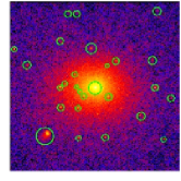
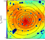
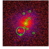
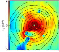
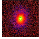
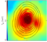
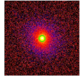
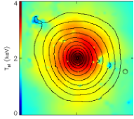
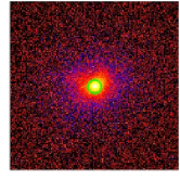
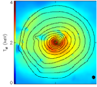
In the left panels of Fig. 1, we report the photon images of our simulated sample. All the images are binned to $2^{\prime\prime}$ pixels and divided by their instrument maps. They are computed in the soft [0.5-2 keV] energy band, to better resolve the presence of small high-emissivity structures or merging objects that otherwise could be hidden by the background. The central panels of Fig. 1 present the spectroscopic-like temperature maps, with the isoflux contours over-plotted. These maps are directly produced from the gas particles in the simulation and show the thermal structure of the systems as would been obtained by ideal X-ray observations of the simulated clusters. On the right panels of the same figures, we plot the histograms of the emission measure, i.e. the sum of the square of the gas density of all the particles inside the box image for $C_{Hot}$, $C_{Pert}$ and $C_{Merg}$ or inside $R_{2500}$ for $C_{Rel1}$ and $C_{Rel2}$, for each bin of temperature and per unit volume. The vertical lines represent the cluster temperature, $T_{2500}$. We notice that the distribution is quite regular and Gaussian only for the relaxed cluster $C_{Rel2}$, while many features are evident for the other systems, revealing their perturbed dynamic state. Nevertheless, we notice that $T_{2500}$ is always lower than the value corresponding to the peak in the emission measure distribution. This is the consequence of fitting with a single temperature the spectra of cluster regions that, as highlighted by the temperature map, show significant gradients or are highly thermally complex (see, e.g. Mazzotta et al., 2004).

3.1 Description of the clusters in the sample

$C_{Hot}$ and $C_{Pert}$ have a quite complex cluster structure. This is evident in the emission measure distributions, which are very broad. The fact that they extend to low temperatures indicates the presence of many cold blobs of gas. Some of them can be seen in the soft X-ray images as bright X-ray blobs distributed around the clusters. The cool nature of these X-ray blobs is confirmed by the temperature maps. To estimate the cluster mass of these complex clusters, we follow the observational approach of excluding from the spatial and spectral analysis all sub-clumps clearly detectable from the soft X-ray image. The excluded regions are shown as green circles in Fig. 1. We know that this procedure partially helps to reduce thermal contamination from colder substructures, however many thermal structures may still remain as they do not produce detectable perturbations in the soft X-ray image.

The largest and hottest cluster, $C_{Hot}$, is actually a still forming object that has not reached the equilibrium state and is undergoing merging events by small substructures.

$C_{Pert}$ presents, in the southern hemisphere, a sub-clump infalling toward the cluster centre and merging with a cold structure located at 1.5 arcmin from the centre.

$C_{Merg}$ appears very relaxed, with no evidence of any peculiar structure both in the photon image and in the temperature map. The elliptical shape of the isoflux contours is the only imprint of a recent major merging happened at $z\approx 0.2$. A further evidence of this recent impact with another big clump comes from the histogram of the emission measure that peaks at two different temperatures ($T\sim 4.1$ keV and $T\sim 3.4$ keV).

The simulated clusters $C_{Rel1}$ and $C_{Rel2}$ have a regular photon image with round isophotes. On the other hand, the temperature map of $C_{Rel2}$ shows the presence of a cold arc in the northern part at $\approx 1$ arcmin from the centre.

4 AN OBSERVATIONAL-LIKE X-RAY ANALYSIS

The event files produced by X-MAS have been then processed using the CIAO 3.0.1 software (see http://cxc.harvard.edu/ciao/) and the calibration files in CALDB 2.23. Surface brightness profiles and spectra have been created and analyzed as described below. In both analyses we exclude the sub-clumps detected in the photon image of $C_{Hot}$ and $C_{Pert}$. Moreover, in all clusters we mask the inner 50 kpc to avoid the influence of the central cooling part. The excluded regions are marked by green circles in the photon images.

4.1 Spatial analysis: brightness profiles

The surface brightness profiles have been extracted from [0.5-5 keV] images that have been corrected thanks to the corresponding instrumental maps.

To build the profile we consider annuli centred on the X-ray peak (in any case, we verified that the off-set from the actual minimum of the cluster potential well is never larger than 2 arcsec) by requiring at least 5000 total counts per bin.

The azimuthal profile has been fitted with a $\beta$-model (Cavaliere & Fusco-Femiano, 1976):

$$S(r)=S_{0}\left[1+\left(\frac{r}{r_{\rm c}}\right)^{2}\right]^{0.5-3\beta}+c_{\rm bkg},$$ (1)

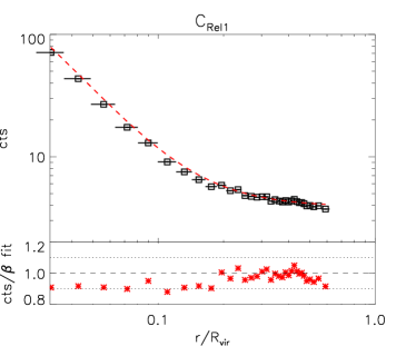
where $r_{c}$ is the core radius, $\beta$ is the power coefficient, and the constant $c_{\rm bkg}$ is the value added to take into account the background present in the image. The best-fit parameters obtained by analyzing our clusters are listed in Table LABEL:tab:param. For all our systems, the deviations between the surface brightness profile and the $\beta$–model fit are less than 10 per cent in the interval between $0.1R_{\rm vir}$ and $1R_{\rm vir}$ (see, e.g., Fig. 2 for cluster $C_{Rel1}$). Nevertheless, the model shows a significant discrepancy in unit of $\sigma$, as shown by the large values of the reduced $\chi^{2}$ reported in Table LABEL:tab:param. Overall, we conclude that the $\beta-$model cannot reproduce the profile of the X-ray emission of the simulated clusters and we find that also a double $\beta$–model is statistically excluded by our data.

Table 2: Best-fit parameters used for the X-ray mass estimators and obtained from the spatial and spectral analysis of the five objects in our sample. $r_{\rm c}$ and $\beta$ are the core radius (in kpc) and the power coefficient of the $\beta$–model; $c_{\rm bkg}$ is the constant representing the background (Eq. 1); $\gamma$ is the polytropic index; $\chi^{2}_{red,\beta}$ and $\chi^{2}_{red,\gamma}$ are the reduced $\chi^{2}$ associated to the $\beta$–model and polytropic relation fitting, respectively; d.o.f. are the degrees of freedom of the fits; $T_{2500}$ is the spectroscopic temperature calculated inside $R_{2500}$; $\sigma_{2500}$ is the associated error at 68 per cent confidence level; $\chi^{2}_{red}$ is the reduced $\chi^{2}$, evaluating the goodness of the spectral fit; $r_{\rm s,NFW}$ and $c_{\rm NFW}$ and $r_{\rm s,RTM}$ and $c_{\rm RTM}$ are the scale radius (in kpc) and the concentration of the NFW and RTM mass model, respectively.

	$C_{Hot}$	$C_{Pert}$	$C_{Merg}$	$C_{Rel1}$	$C_{Rel2}$
$r_{\rm c}$	85$\pm$2	101$\pm$6	61$\pm$2	21$\pm$1	14$\pm$1.5
$\beta$	0.56$\pm$0.01	0.44$\pm$0.01	0.62$\pm$0.01	0.52$\pm$0.01	0.56$\pm$0.01
$c_{\rm bkg}$	1.78	4.30	3.91	3.88	4.06
$\chi^{2}_{red,\beta}$ (d.o.f.)	4.2 (13)	3.9 (70)	7.6 (44)	5.3 (39)	11.7 (29)
$\gamma$	1.09$\pm$0.03	1.11$\pm$0.15	1.10$\pm$0.02	1.11$\pm$0.04	1.06$\pm$0.03
$\chi^{2}_{red,\gamma}$ (d.o.f.)	1.4 (6)	0.6 (4)	0.5 (10)	0.9 (5)	2.6 (3)
$T_{2500}$	11.18	3.87	3.76	3.39	2.64
$\sigma_{2500}$	$\pm 0.48$	$\pm 0.36$	$\pm 0.08$	$\pm 0.12$	$\pm 0.08$
$\chi^{2}_{red}$ (d.o.f.)	0.51 (45)	0.36 (39)	0.44 (103)	0.31 (30)	0.37 (80)
$r_{\rm s,NFW}$	668$\pm$47	350$\pm$100	216$\pm$103	82$\pm$45	252$\pm$38
$c_{\rm NFW}$	6.0$\pm$0.3	6.1$\pm$2.5	8.6$\pm$2.3	16.2$\pm$7.9	7.2$\pm$1.0
$r_{\rm s,RTM}$	693$\pm$112	351$\pm$121	148$\pm$69	41$\pm$20	226$\pm$70
$c_{\rm RTM}$	7.5$\pm$1.1	7.4$\pm$5.3	14.3$\pm$5.4	36.2$\pm$8	9.9$\pm$3.3

Figure 2: The surface brightness profile (in units of photon counts) of the simulated cluster $C_{Rel1}$. Open squares represent the values extracted from the X-ray analysis, the horizontal bars correspond to the bin sizes. The dashed curve is the corresponding best-fit $\beta$-model, with $\beta=0.52$ and $r_{c}=21$ kpc (= 0.013 $R_{\rm vir}$). The bottom panel shows the ratio between the profile from the X-ray analysis and the best-fit $\beta$-model.

4.2 Spectral analysis

To measure the overall temperature we extract spectra from circular regions centred on the cluster centre and with a radius $r=R_{2500}$. To calculate the temperature profiles we extract spectra from annular regions for which the net counts (i.e. belonging to the cluster) are greater than 5000 and are at least 25 per cent or the total counts. As in the spatial analysis the regions marked by green circles in Fig. 1 are excluded from the spectral analysis.

For each region, the ancillary response file (ARF) and the redistribution matrix file (RMF), weighted by the X-ray brightness in the [0.3–2 keV] energy range, are computed by using the CIAO tools mkwarf and mkrmf. Source spectra are extracted from the event file, re-binned and analyzed in the [0.5–6 keV] band. Background spectra are extracted from the background event file for the same source regions. A thermal model (mekal) absorbed by the Galactic column density is fitted to the data by using the $\chi^{2}$ statistic in the XSPEC package (Arnaud, 1996). The only free parameters are the gas temperature and the normalization, being Galactic absorption $N_{\rm H}$, redshift $z$ and metallicity $Z$ fixed to the input values adopted in the X-MAS run: $N_{\rm H}=5\times 10^{20}$ cm^-2, $z=0.175$ and $Z=0.3Z_{\odot}$.

In Table LABEL:tab:param, we quote the best-fit values of the spectroscopic temperature, $T_{2500}$, with the corresponding 68% confidence level error $\sigma_{2500}$. These value are also shown as vertical lines in the right panels of Fig. 1.

4.3 Deprojection results

To compute the mass through the equation of the hydrostatic equilibrium as described in the next section, we need to recover the three-dimensional profiles of the gas temperature and density by deprojecting the quantities measured in the X-ray spectral analysis. We adopt the deprojection technique presented in Ettori et al. (2002), that is described briefly here. For each annulus with luminosity $L_{\rm ring}$, a single thermal model is fitted to the projected spectrum as described in the previous section, giving the temperature $T_{\rm ring}$. By using the geometrical corrections discussed in Kriss et al. (1983), the photon-weighted, projected-on-the-sky measured quantities are converted to the values expected in spherical shells by the relations:

$$\begin{array}[]{l}n_{\rm e}=\left[({\bf Vol}^{T})^{-1}\#(EI/0.82)\right]^{1/2}\ ,\\ \epsilon=({\bf Vol}^{T})^{-1}\#L_{\rm ring}\ ,\\ T=({\bf Vol}^{T})^{-1}\#(L_{\rm ring}T_{\rm ring})\,/\,\epsilon\ ,\end{array}$$ (2)

where we define the electron density $n_{\rm e}$ in terms of proton density $n_{\rm p}$ as $n_{\rm e}=n_{\rm p}/0.82$, the Emission Integral is $EI=\int n_{\rm e}n_{\rm p}dV=0.82\int n_{\rm e}^{2}dV=K\times 4\pi d_{\rm ang}^{2}(1+z)^{2}\times 10^{14}$, $K$ is the normalization of the mekal model, and the symbol $\#$ represents the “matrix product” operator. The matrix ${\bf Vol}$ contains the values of the fractions of the spherical volume of a shell seen at each ring. [The notation $({\bf Vol}^{T})^{-1}$ indicates that the matrix is firstly transposed and then inverted]. The outputs are then the measurements of the electron density and plasma temperature in each volume shell with given inner and outer radii.

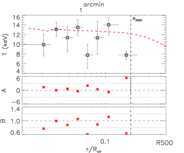
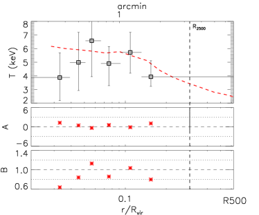
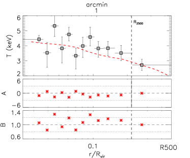
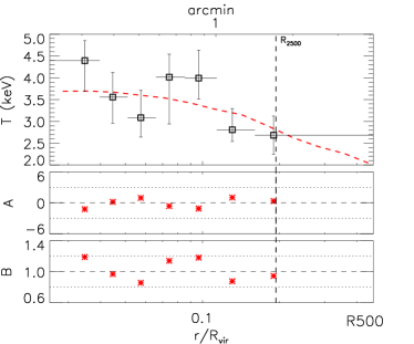
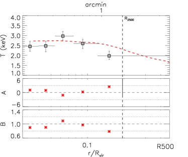
We compare in Fig.3 the deprojected temperature measure, $T$, with the three-dimensional mass-weighted estimate, $T_{\rm mw}$, resulting from the simulations. The mass-weighted temperature is estimated directly from the hydrodynamic simulations as $T_{\rm mw}=\int mTdV/\int mdV$, where $m$ is the mass of each gas particle. $T_{\rm mw}$ is the proper temperature value we should use in the hydrostatic equilibrium equation to derive the mass (Mathiesen & Evrard, 2001, see also Section 4.4). Since the clusters in our sample have an azimuthally quite symmetric thermal structure, we find that their $T_{\rm mw}$ profile is not very dissimilar from the $T_{\rm spec}$ one, even if in the outer regions the values obtained in the X-ray analysis are systematically lower. A more quantitative comparison can be done by looking at the bottom graphs of each panel, where we show a parameter similar to the one defined in Section 4.2: $A\equiv(T-T_{\rm mw})/\sigma_{\rm spec}$, where now the temperatures are three-dimensional quantities, and the ratio between the deprojected temperature and the mass-weighted temperature: $B\equiv(T/T_{\rm mw})$. We find that, while $|A|\la 3$ up to $R_{500}$ for all the objects, $B$ indicates that the spectroscopic temperature is within 20 per cent of $T_{\rm mw}$, with implications on the mass estimates (Mathiesen & Evrard, 2001; Vikhlinin et al., 2005, see Section 5.1).

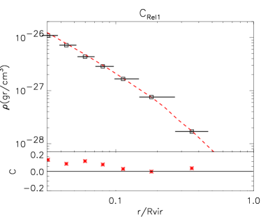
Just as an example, in Fig. 4 we compared to the true profile $\rho_{\rm sim}$, of the simulated cluster $C_{Rel1}$ (dashed line), with the gas density obtained from the deprojection technique used. We find a good agreement for $r/R_{\rm vir}>0.1$, result that holds also for the other clusters.

Figure 3: Deprojected temperature profile for $C_{Hot}$, $C_{Pert}$, $C_{Merg}$, $C_{Rel1}$, and $C_{Rel2}$. The dashed line represents the profile for the three-dimensional mass-weighted temperature $T_{\rm mw}$ as obtained from the hydrodynamic simulation. The open squares are the values extracted from the X-ray analysis, the vertical bars are $1\sigma$ errors ($\sigma_{\rm spec}$), while the horizontal ones correspond to the bin sizes. The bottom graphs in each panel show quantities related to the differences between the two temperatures: $A\equiv(T-T_{\rm mw})/\sigma_{\rm spec}$ and $B\equiv(T/T_{\rm mw})$. The dotted lines indicate $A=(-3,3)$ and $B=(0.8,1.2)$.

Figure 4: Deprojected density profile of $C_{Rel1}$. The red dashed line represents the density profile as obtained from the hydrodynamic simulation ($\rho_{\rm sim}$). The dots are the values extracted from the X-ray analysis ($\rho$), the vertical bars (having sizes comparable to the dots) are $1\sigma$ errors, while the horizontal ones correspond to the bin sizes. The bottom panel shows the relative differences between the true values of the simulation and the derived ones, $C\equiv(\rho_{\rm sim}-\rho)/\rho_{\rm sim}$.

4.4 X-ray estimates of the gravitational mass

The “true” mass profile, $M_{\rm sim}(<r)$, of the simulated objects, obtained by summing all the masses of the particles inside a sphere of radius $r$, can be now compared to several different X-ray mass estimators, $M_{\rm est}$, that we discuss below.

• $M_{\rm est}$ from the direct application of the hydrostatic equilibrium equation: $M_{\rm HE}$

  This method (as discussed in Ettori et al., 2002) makes use of the hydrostatic equilibrium (HE) equation under the assumption of spherical symmetry to estimate the total gravitating mass:

  $$M_{\rm HE}(<x)=-\frac{kT(x)xR_{\rm vir}}{G\mu m_{\rm p}}\left(\frac{d\ln\rho}{d\ln x}+\frac{d\ln T}{d\ln x}\right)\ ,$$ (3)

  where $G$ is the gravitational constant, $\mu$=0.59 is the mean molecular weight in a.m.u., $m_{\rm p}$ is the proton mass, $k$ is the Boltzmann constant, $x\equiv r/R_{\rm vir}$ and $T$ and $\rho$ are the deprojected 3D profiles. The equation is applied directly to the deprojected data by estimating the derivatives with respect to $\ln x$ of $\ln(\rho\times T)$ without any further smoothing of the measured data points. The HE equation is based on simple assumptions: sphericity, static gravitational potential and isotropic velocity field. Recent studies have shown how the latter hypothesis is often not satisfied inside both simulated clusters (see, e.g., Rasia et al., 2004; Kay et al., 2004) and observed ones (see, e.g., Zhang et al., 2005; Dupke & Bregman, 2005). Rasia et al. (2004) suggested that in order to correctly compute the total mass, the gas velocity has to be taken into account, because it is a relevant component of the total energy equipartition between gas and dark matter. The more general model describing the gas dynamical equilibrium can be then written as:

  $$M_{HE,v}(<x) =-\frac{kT(x)xR_{\rm vir}}{G\mu m_{\rm p}}\left[\frac{d\ln\rho}{d\ln x}+\frac{d\ln T}{d\ln x}\right]$$ (4)

  $$-\frac{\sigma_{r}^{2}xR_{\rm vir}}{G}\left[\frac{d\ln\rho}{d\ln x}+\frac{d\ln\sigma_{r}^{2}}{d\ln x}+2\beta_{v}(x)\right],$$

  where $\beta_{v}(\equiv 1-\sigma_{t}^{2}/2\sigma_{r}^{2})$ is the gas velocity anisotropy parameter and $\sigma_{r}$ and $\sigma_{t}$ are the gas radial and tangential velocity dispersions, respectively. Since some years, velocity fields have been studied in simulated cluster as bulk motion (see, e.g. Norman & Bryan, 1999) or turbulent motions (see, e.g. Dolag et al., 2005; Vazza et al., 2006). Nevertheless, robust observational measurements of $\beta_{v}$ and, more in general, of the gas bulk motions are difficult (see, e.g., Dupke & Bregman, 2005) and due to the failure of Suzaku satellite spectrometer, we have to wait the new generation of high spectroscopic resolution X-satellites to determine the cluster velocity structure. In the present analysis, we evaluate the second part of Eq. 4 directly from the simulations.

• $M_{\rm est}$ using $\beta-$model and polytropic temperature profile: $M_{\beta,\gamma}$

  Assuming that the gas density profile is described by a $\beta-$model and that it is related to the temperature through the polytropic relation ($T\propto\rho^{\gamma-1}$, with $1\leq\gamma\leq 5/3$), Eq. 3 can be written as (see, e.g., Henriksen & Mushotzky, 1986):

  $$M_{\beta,\gamma}(<x) = -\frac{kT(x)\ x}{G\mu m_{\rm p}}\left(\frac{d\ln\rho}{d\ln x}+\frac{d\ln T}{d\ln x}\right)$$ (5)

  $$= \frac{3\ \beta\gamma\ T_{0}\ r_{\rm c}}{G\mu m_{\rm p}}\frac{x_{\rm c}^{3}}{(1+x_{\rm c}^{2})^{\alpha}}$$

  $$= \frac{0.757\times 10^{14}}{\mu}\beta\gamma T_{0}r_{\rm c}\frac{x_{\rm c}^{3}}{(1+x_{\rm c}^{2})^{\alpha}}\ M_{\odot},$$

  where $x_{\rm c}\equiv r/r_{\rm c}$, $r_{\rm c}$ is the core radius (in units of $h_{70}^{-1}$ Mpc), $\alpha=1.5\beta(\gamma-1)+1$ and $T_{0}$ is the central temperature in keV.

• $M_{est}$ from an isothermal $\beta-$model: $M_{\beta}$

  Rather than relating the gas density and temperature accordingly to the polytropic law, an isothermal gas is here assumed. The total mass is then obtained from Eq. 5 by imposing $\gamma=1$ and $T_{0}=T_{500}$ (reported in Table LABEL:tab:param).

• $M_{est}$ through analytic mass models: $M_{\rm NFW}$ and $M_{\rm RTM}$

  This method, widely adopted in the reconstruction of the X-ray mass profile (see, e.g., Allen et al., 2002), makes use of functional forms of the radial mass distribution obtained from numerical simulations. The derived gravitational potential is combined with the deprojected gas density profile to recover a temperature profile through the numerical inversion of the HE equation. A $\chi^{2}$ distribution is then obtained by a grid of values for the two free parameters of the mass model (the scale radius $r_{\rm s}$ and the concentration parameter $c$) by estimating the deviation between the numerical temperature profile and the deprojected one. The errors on the best-fit parameters are inferred from the distribution of the $\chi^{2}$ values.

  As functional forms of the mass profile, we have used here those proposed by Navarro et al. (1997) (hereafter NFW) and by Rasia et al. (2004) (hereafter RTM), which read

  $$M_{\rm NFW}(<x) \propto \log(1-x\,c_{\rm NFW})-\frac{x\,c_{\rm NFW}}{1-x\,c_{\rm NFW}^{3}}\ ,$$

  $$M_{\rm RTM}(<x) \propto \left[\frac{(x\,c_{\rm RTM}+2)}{x\,c_{\rm RTM}+1}^{1/2}-2\right],$$ (6)

  respectively, with $x\equiv r/R_{\rm vir}$.

  The values of the corresponding best-fit parameters for our set of simulated clusters are reported in Table LABEL:tab:param.

5 Results on the mass profiles

Table 3: Deviations between the masses calculated by using the different mass estimators $M_{\rm est}$ (see their description in the text) and the true mass $M_{\rm sim}$ as directly obtained from the simulated clusters, in units of the estimators errors: $|M_{\rm est}-M_{\rm sim}|/\sigma_{\rm est}$. In the case of discrepancies greater than 1 $\sigma_{\rm est}$ we report in parenthesis the value of the percentage difference: $(|M_{\rm est}-M_{\rm sim}|/M_{\rm est})\times 100$. The values are computed at $R_{2500}$ and extrapolated to $R_{500}$ for $M_{\beta}$, $M_{\beta,\gamma}$, $M_{\rm RTM}$, and $M_{\rm NFW}$.

	$C_{Hot}$	$C_{Pert}$	$C_{Merg}$	$C_{Rel1}$	$C_{Rel2}$
	${\bf R_{2500}}$
$M_{HE}$	1	1	1	1	1
$M_{HE,v}$	1	1	1	1	1
$M_{\beta,\gamma}$	$>10$ (47)	$>10$ (49)	$>10$ (23)	$>10$ (37)	$>10$ (36)
$M_{\beta}$	$>10$ (43)	$>10$ (58)	$>10$ (24)	$>10$ (35)	$>10$ (31)
$M_{\rm NFW}$	1	1	1	2 (20)	3 (24)
$M_{\rm RTM}$	2 (13)	1	1	2 (20)	5 (32)
	${\bf R_{500}}$
$M_{\beta,\gamma}$	$>10$ (52)	4 (45)	7 (28)	9 (42)	7(37)
$M_{\beta}$	10 (44)	10 (51)	10 (17)	¿10 (31)	¿10(25)
$M_{\rm NFW}$	1	1	1	2 (35)	3(46)
$M_{\rm RTM}$	3 (56)	1	1	3 (27)	4(81)

Figure 5: Ratios between the mass profiles derived from the X-ray analysis, $M_{\rm est}$, and the true mass profile of the simulated cluster, $M_{\rm sim}$ for our galaxy clusters: $C_{Hot}$, $C_{Pert}$, $C_{Merg}$, $C_{Rel1}$ and $C_{Rel2}$. The vertical lines indicate $R_{2500}$. The red asterisks and the green diamonds represent the mass derived by assuming the hydrostatic equilibrium, $M_{HE}$ (Eq. 3) and $M_{HE,v}$ (Eq. 4), respectively. The solid blue and the thick cyan lines refer to the $\beta-$model, $M_{\beta}$, and $\beta-$model plus polytropic relation, $M_{\beta,\gamma}$ (Eq.5), respectively. The green and magenta dashed lines show the masses derived by assuming the analytic profiles, $M_{\rm NFW}$ and $M_{\rm RTM}$, respectively (Eq.6). The measured errors (1 $\sigma$ ) on the mass estimators are represented by vertical error bars or thin solid lines in the case of $M_{\rm NFW}$ and $M_{\rm RTM}$.

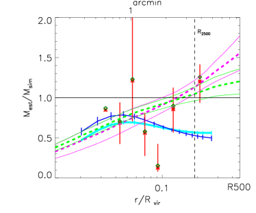
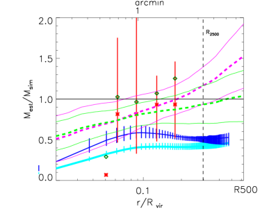
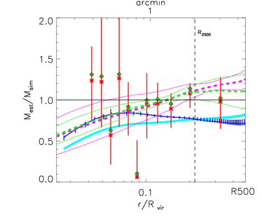
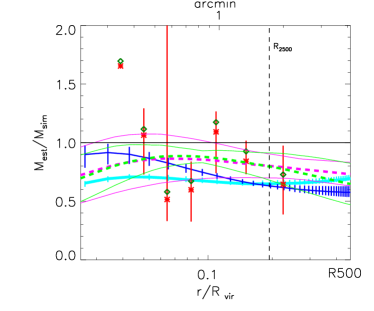
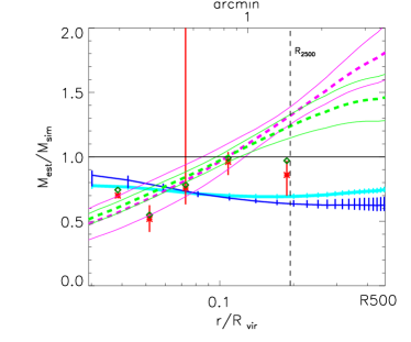
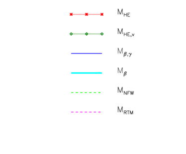
The ratios between the mass profiles reconstructed by using all these methods, $M_{\rm est}$, and the true mass profiles as extracted by simulated clusters, $M_{\rm sim}$, are shown in Fig. 5. Note that the uncertainties relative to the X-ray mass measurements as shown in Fig. 5 decrease indeed in relation to the dynamic state of the cluster, with the largest errors being associated to the first three objects ($C_{Hot}$, $C_{Pert}$, $C_{Merg}$) and the smallest ones to the most relaxed systems, $C_{Rel1}$ and $C_{Rel2}$. The vertical dashed lines refer to the radii corresponding to $R_{2500}$. In Table LABEL:tab:mass we quote the differences between the true mass and the mass estimates in units of the error at this radius and at $R_{500}$, where $M_{\beta}$, $M_{\beta,\gamma}$, $M_{\rm RTM}$, and $M_{\rm NFW}$ need to be extrapolated. In the case of discrepancies greater than 1 $\sigma$ error we report also the percentage difference in parenthesis.

We summarize here our results and, where needed, discuss the main reasons for the observed discrepancies between the estimated X-ray mass and the total mass distribution.

• The mass profile obtained from the HE equation, $M_{HE}$, dependent upon the measured temperature profile (see Fig. 3). Large errors on, and irregular radial distribution of, the temperature values induce large scatter on the reconstructed $M_{HE}$ measurements. As clear from the figure, this mass estimator produces large errors mainly related to the background level. For this reason most of these measurements are within $1\sigma$ from the expected values, even in objects that are still undergone to some (minor) mergers and for which the hydrostatic equilibrium might have not been reached yet ($C_{Hot}$ and $C_{Pert}$). If we focus only on the best fit value, we notice that, in the case of $C_{Hot}$, $M_{HE}$ overestimates the true mass due to the steepness of the temperature profile at $R_{2500}$ owing to the wrong measurement of temperature profile in the last bin. On the other hand, it underestimates the true mass in relaxed objects (see Fig. 5).

  The effect of the gas bulk motions are always smaller 10 per cent, excluding for the cluster $C_{Pert}$. In this case the kinetic energy is significant mostly because of the entering merging blob in the South and can still contribute between 20 and 30 per cent to the total mass measurements. The neglected kinetic pressure term can partially compensate for the present best fit deviations in relaxed systems.

• The analytic masses, $M_{\rm NFW}$ and $M_{\rm RTM}$, are reconstructed starting from the hydrostatic equilibrium equation, therefore they follow the behaviour of the $M_{HE}$ profile, but they have smaller errors. Nevertheless, we notice that the statistical errors are still too high to show significant mass discrepancies (Fig. 5).

• The $\beta$–model gives the worse mass reconstruction with mass discrepancies $>10\sigma$ significant (see also Bartelmann & Steinmetz, 1996; Muanwong et al., 2002; Rasia et al., 2004; Borgani et al., 2004; Rasia et al., 2005). $M_{\beta,\gamma}$ is 5-10 per cent lower than $M_{\beta}$ in the outer regions ($r>R_{500}$) owing to the use of a polytropic law to describe the relation between the measured temperature and density profiles. Here we note that, in our simulated clusters, the correlation between $\ln T(r)$ and $\ln\rho(r)$ cannot be reproduced by a single linear relation and requires the polytropic index $\gamma=1+\ln T/\ln\rho$ to vary between 1.1 and 1.2 moving outwards. The use of an inappropriate assumption on the functional form of the temperature profile propagates to the mass measurements making them less accurate than the estimates done with the isothermal $\beta$–model. The main sources of the difference for these models are (i) the poorness of the $\beta$–model in describing the density profile, (ii) the incorrect assumption of isothermality or above all of the polytropic relation, and (iii) the uncertain determination of the $\beta$–model parameters (which we will discuss in the next subsection).

Looking at the behaviour of each single cluster, we notice that, even for the dynamically disturbed objects, the central values of the total mass can be recovered within 20-30 per cent at $R_{2500}$, the situation being worse at $R_{500}$.

5.1 On the NFW concentration and $\beta$ parameter

The computation of the mass directly depends on the values of the best-fit parameters, like the NFW concentration, $c_{\rm NFW}$, or the $\beta$ value in the $\beta-$model. The former is evaluated from the mass functional form that better reproduces the observed temperature profile at $r>50$ kpc. The inner 50 kpc are also excluded in the spatial analysis that provides an estimate of $\beta$, to avoid any influence from the central cooling region where a too large amount of cool gas concentrates in our simulated clusters (see, e.g., Borgani et al., 2004).

We investigate here how the measurement of these parameters depends upon the considered radial range. When we also include in the analysis the central region within 50 kpc, the concentration parameter becomes larger, but the reduced $\chi^{2}$ also increases. The cluster $C_{Merg}$ is an example: $c_{\rm NFW}$ rises from 8.6 to 28 and the reduced $\chi^{2}$ from 0.9 to 2.6. On the contrary, the value for $\beta$ does not vary significantly (the most relevant deviation is for $C_{Pert}$, where $\beta$ changes from 0.56 to 0.47). Also in the spatial fit of the surface brightness, when including the inner 50 kpc region the reduced $\chi^{2}$ of the fit increases. While this systematic effect can be easily handled from an observational point of view, the influence of the outer end of the radial range is limited by the field of view of the detector and by the background. From a direct fit of the data from the simulations, we find that both parameters depend strongly upon the adopted outer radius, and that, while $c_{\rm NFW}$ decreases, $\beta$ increases when larger radii are considered (see also Navarro et al., 1995; Bartelmann & Steinmetz, 1996; Borgani et al., 2004). The same trend occurs when we fit an NFW and a $\beta-$model to the density profile. For example, we measure $c_{\rm NFW}\approx 5.3$ by fitting the simulated density profile of $C_{Merg}$ out to the virial radius (see Table 1), while $c_{\rm NFW}\approx 7.0$ if we limit the fit to the region mapped in the Chandra field-of-view and $c_{\rm NFW}\approx 8.6$ if we use the deprojected temperature profile.

In summary, the concentration parameter and the $\beta$ value are affected by both the method used to derive them and the radial interval over which they are measured. These two limitations have the same effect: the observed $c_{\rm NFW}$ and $\beta$ will be always higher and lower, respectively, than the values directly derived by fitting the density of simulated clusters up to the virial radius.

5.2 Effect of the background level

Table 4: The same of Table LABEL:tab:mass but derived using a background level 100 lower that the Chandra value (see text in Sect.5.2).

	$C_{Hot}$	$C_{Pert}$	$C_{Merg}$	$C_{Rel1}$	$C_{Rel2}$
	${\bf R_{2500}}$
$M_{HE}$	1	1	7 (30)	$>10$ (30)	$>10$ (28)
$M_{HE,v}$	1	1	6 (24)	8 (22)	9 (17)
$M_{\beta,\gamma}$	$>10$ (46)	$>10$(33)	$>10$ (26)	$>10$ (40)	$>10$ (37)
$M_{\beta}$	$>10$ (44)	8 (30)	$>10$ (16)	$>10$ (31)	$>10$ (26)
$M_{\rm NFW}$	8 (19)	4 (34)	$>10$ (27)	$>10$ (13)	5(10)
$M_{\rm RTM}$	5 (18)	5 (31)	$>10$ (19)	6 (16)	4 (11)
	${\bf R_{500}}$
$M_{HE}$	1	1	5	4 (15)	9 (32)
$M_{HE,v}$	2 (30)	1	3	1	4 (13)
$M_{\beta,\gamma}$	$>10$(44)	11 (35)	$>10$ (30)	$>10$ (45)	$>10$ (37)
$M_{\beta}$	$>10$(42)	2 (9)	6 (7)	$>10$ (25)	$>10$ (19)
$M_{\rm NFW}$	2 (10)	3 (40)	$>10$ (46)	7 (7)	3 (13)
$M_{\rm RTM}$	1	5 (30)	$>10$ (24)	3 (6)	4 (8)

In the previous analysis, we follow an observational approach to recover the mass from Chandra observations. Mainly due to the relatively high background level of Chandra , this results in statical errors for the temperature profile that, in some cases, are too large to be able to show significant mass discrepancies between the recovered and true mass in Fig. 5. In prevision of future missions that will be able better control and reduce the instrumental noise, we reanalyzed the same clusters using Chandra observations for which the background accumulation time has been reduced by a factor of 100 implying that the effective background has been reduced by a factor of 100. Using these new data set we are able to extract cluster signal to larger radii than before (we remind that we restricted our analysis to all the annuli with at least 5000 net counts and with a flux from the source greater that 25% of the total flux) that easily extend beyond $R_{500}$. As before, we find that the all the best fit values of the estimated X-ray mass underestimate the true mass by a remarkable amount: by 20–40 per cent using $M_{\beta}$ and by $\la 20$ per cent using $M_{HE}$ or the analytic functional forms. Due to reduced statistical error, we can now see that these discrepancies are in many cases statistically significant to more than $3\sigma$ as clearly shown in Table LABEL:tab:mass2. It is worth saying that, in contrast with Table LABEL:tab:mass in this case the values at $R_{500}$ are not extrapolation but measurements.

It is also worth noting the behaviour of the analytic masses in comparison with the case of normal background reproduced (Table LABEL:tab:mass): being the errors largely reduced the true mass is always out of 3$\sigma$ and it comes to be strongly underestimated. The masses recovered by the hydrostatic equilibrium present the same characteristic, but for the clusters showing a perturbed dynamical state because they are still conserving large error bars. In particular, we investigated the reason of the understimation of $M_{\rm HE}$ and we find that half of the total discrepancy is provided by neglecting the kinetic energy still present as bulk motions of the intra-cluster medium. The remaining deviation arises from a systematically lower measurement of the representative gas temperature. In other words, in these conditions of very low background, the deprojected spectral value is systematically lower than the mass-weighted estimate from numerical simulations by about 10 per cent, suggesting that a proper use of well-defined gas temperature values in the hydrostatic equilibrium equation should allow a more rigorous measurements of the total mass profile.

6 SUMMARY AND DISCUSSION

We have investigated the bias on the X-ray mass estimates with mock long Chandra exposures of five galaxy clusters obtained from high-resolution hydrodynamic simulations using an observational-like approach. The five objects have a spectroscopic-like temperature between $2.7$ and $11.4$ keV, and are at redshift $z=0.175$ to fit their $R_{500}$ within Chandra ACIS-S3 chip. They are characterized by different dynamical states: two objects are perturbed, one had a recent major merging, and two are fairly relaxed. These simulated clusters are processed with our X-ray Map Simulator, X-MAS , to produce realistic X-ray event files and images that are analyzed with the goal of measuring the total mass profile. To evaluate the systematic effects present both in the assumptions of hydrostatic equilibrium and of the $\beta$–model and in the observational techniques adopted in recovering the mass measurement, we compare the estimated mass profiles to the ones directly measured in the hydrodynamic simulations used as input for our analysis.

The main results, shown in Fig. 5 and quoted in Tables LABEL:tab:mass and  LABEL:tab:mass2, can be summarized as follows.

• Due to the relatively high statistical errors mainly connected with the high background level of the Chandra observations, the HE equation seems to recover, within the errors, the true cluster mass profile of the simulated clusters. This partially holds also for the analytic mass models NFW and RTM. If however we reduce the background level by a factor of 100, we immediately see, to a confidence level $>3\sigma$, that the reconstructed masses using this technique are underestimated by 20% (see Table LABEL:tab:mass2). In this case, we find that the neglected kinetic pressure term can compensate for about half of the observed deviations in relaxed systems, while the other half is due to the underestimated measurement of the temperature in comparison to the mass-weighted one.

• The mass measurements reconstructed via the $\beta$–model are the worst among the models considered in the present work since they show a systematic underestimate, with typical deviations of about $40$ per cent at $R_{2500}$ and $R_{500}$. $M_{\beta,\gamma}$ is 5-10 per cent lower than $M_{\beta}$ in the outer regions ($r>R_{500}$) owing to the use of a too simplistic polytropic equation state that relates temperature and density profiles. The use of the polytropic functional form of the temperature profile makes the mass measurements less accurate than that provided from the isothermal $\beta$–model. The other sources of biases for the $\beta$–model mass come from (i) its inaccurate description of the density profile, (ii) the poor determination of the parameters describing the spatially-extended X-ray emission.

• A systematic effect, that influences the determination of the mass through the $\beta$–model mass and the analytic formulae, is also produced by the radial interval considered to constrain the value of $\beta$ of the $\beta-$model and the concentration parameter in the NFW formula. We stress that the observed $\beta$ and $c_{\rm NFW}$ will be always lower and higher, respectively, than the values derived directly by fitting the density of simulated clusters out to the virial radius (see, e.g. the observational evidence in Vikhlinin et al., 1999; Neumann, 2005).

• We conclude that the mass estimates based on the hydrostatic equilibrium equation in combination with the temperature profile and those of the analytic fits (NFW or RTM) provide a more robust mass estimate than the ones based on the $\beta-$model.

It is important to remarke that the data analysis performed in this paper has been made under ideal conditions. In fact we assumed to know precisely both the background and the instrument response. Furthermore we used very long exposures for all the simulated observations reaching a large number of net counts. It is clear that the uncertainties in the background and instrument response which are inevitably present in real observations (as well as shorter exposures) may easily make these discrepancies larger. Moreover we remind that the physics adopted in the simulations biases our results on the temperature and density profiles more significantly when the thermal structure of the X-ray emitting plasma is more complex, in the sense that it becomes problematic and ambiguous to represent the average properties of a gas which presents a wide range in emission measures and temperatures.

Finally, we notice that these systematic effects on the X-ray total mass propagate to the constraints on the cosmological parameters obtained by using clusters as probes of the matter distribution in the Universe. At the present, statistical uncertainties associated to the paucity of available high–redshift cluster samples are comparable to systematic uncertainties arising from biases in cluster mass estimates (see, e.g., Rosati et al., 2002), as those discussed in this paper. As larger samples of distant clusters will be available in the near future, it is clear that such systematics will start to dominate over statistical errors. In this respect, extensive analyses, like the one presented here, will be of crucial relevance to quantify possible biases in any procedure of cluster mass estimate. However, the size of systematic biases and uncertainties, as calibrated from hydrodynamic simulations, depends on the physical processes included in the simulations themselves. This highlights the fundamental role played by an accurate numerical treatment of the complex physics of the ICM to calibrate clusters from hydrodynamic simulations as precision tools for cosmology.

References

- Allen et al. (2002) Allen S. W., Schmidt R. W., Fabian A. C., 2002, MNRAS, 335, 256
- Anders & Grevesse (1989) Anders E., Grevesse N., 1989, Geochimica et Cosmochimica Acta, 53, 197
- Arnaud (1996) Arnaud K. A., 1996, in ASP Conf. Ser. 101: Astronomical Data Analysis Software and Systems V XSPEC: The First Ten Years. p. 17
- Balland & Blanchard (1997) Balland C., Blanchard A., 1997, ApJ, 487, 33
- Bartelmann & Steinmetz (1996) Bartelmann M., Steinmetz M., 1996, MNRAS, 283, 431
- Borgani et al. (2005) Borgani S., et al., 2005, preprint, astro-ph/0512506
- Borgani et al. (2004) Borgani S., et al., 2004, MNRAS, 348, 1078
- Cavaliere & Fusco-Femiano (1976) Cavaliere A., Fusco-Femiano R., 1976, A&A, 49, 137
- Cowie et al. (1987) Cowie L. L., Henriksen M., Mushotzky R., 1987, ApJ, 317, 593
- Dolag et al. (2004) Dolag K., Jubelgas M., Springel V., Borgani S., Rasia E., 2004, ApJL, 606, L97
- Dolag et al. (2005) Dolag K., Vazza F., Brunetti G., Tormen G., 2005, MNRAS, 364, 753
- Dorman et al. (2003) Dorman B., Arnaud K. A., Gordon C. A., 2003, AAS/High Energy Astrophysics Division, 7,
- Dupke & Bregman (2005) Dupke R. A., Bregman J. N., 2005, ApJS, 161, 224
- Eke et al. (1996) Eke V. R., Cole S., Frenk C. S., 1996, MNRAS, 282, 263
- Ettori et al. (2002) Ettori S., De Grandi S., Molendi S., 2002, A&A, 391, 841
- Evrard et al. (1996) Evrard A. E., Metzler C. A., Navarro J. F., 1996, ApJ, 469, 494
- Gardini et al. (2004) Gardini A., Rasia E., Mazzotta P., Tormen G., De Grandi S., Moscardini L., 2004, MNRAS, 351, 505
- Henriksen & Mushotzky (1986) Henriksen M. J., Mushotzky R. F., 1986, ApJ, 302, 287
- Jubelgas et al. (2004) Jubelgas M., Springel V., Dolag K., 2004, MNRAS, 351, 423
- Kay et al. (2004) Kay S. T., Thomas P. A., Jenkins A., Pearce F. R., 2004, MNRAS, 355, 1091
- Kriss et al. (1983) Kriss G. A., Cioffi D. F., Canizares C. R., 1983, ApJ, 272, 439
- Mathiesen & Evrard (2001) Mathiesen B. F., Evrard A. E., 2001, ApJ, 546, 100
- Mazzotta et al. (2004) Mazzotta P., Rasia E., Moscardini L., Tormen G., 2004, MNRAS, 354, 10
- Muanwong et al. (2002) Muanwong O., Thomas P. A., Kay S. T., Pearce F. R., 2002, MNRAS, 336, 527
- Navarro et al. (1995) Navarro J. F., Frenk C. S., White S. D. M., 1995, MNRAS, 275, 720
- Navarro et al. (1997) Navarro J. F., Frenk C. S., White S. D. M., 1997, ApJ, 490, 493
- Neumann (2005) Neumann D., 2005, A&A, 439, 465
- Norman & Bryan (1999) Norman M. L., Bryan G. L., 1999, LNP Vol. 530: The Radio Galaxy Messier 87, 530, 106
- Rasia et al. (2005) Rasia E., Mazzotta P., Borgani S., Moscardini L., Dolag K., Tormen G., Diaferio A., Murante G., 2005, ApJL, 618, L1
- Rasia et al. (2004) Rasia E., Tormen G., Moscardini L., 2004, MNRAS, 351, 237
- Rosati et al. (2002) Rosati P., Borgani S., Norman C., 2002, ARA&A, 40, 539
- Sarazin (2002) Sarazin C. L., 2002, The Physics of Cluster Mergers. ASSL Vol. 272: Merging Processes in Galaxy Clusters, pp 1–38
- Schindler (1996) Schindler S., 1996, A&A, 305, 756
- Springel (2005) Springel V., 2005, MNRAS, 364, 1105
- Springel & Hernquist (2002) Springel V., Hernquist L., 2002, MNRAS, 333, 649
- Springel & Hernquist (2003) Springel V., Hernquist L., 2003, MNRAS, 339, 289
- Springel et al. (2001) Springel V., Yoshida N., White S., 2001, New Astronomy, 6, 79
- Tormen et al. (1997) Tormen G., Bouchet F., White S., 1997, MNRAS, 286, 865
- Vazza et al. (2006) Vazza F., Tormen G., Cassano R., Brunetti G., Dolag K., 2006, ArXiv Astrophysics e-prints
- Vikhlinin (2005) Vikhlinin A., 2005, preprint, astro-ph/0504098
- Vikhlinin et al. (2005) Vikhlinin A., et al., 2005, preprint, astro-ph/0507092
- Vikhlinin et al. (1999) Vikhlinin A., Forman W., Jones C., 1999, ApJ, 525, 47
- Voit (2005) Voit G. M., 2005, Reviews of Modern Physics, 77, 207
- Yoshida et al. (2001) Yoshida N., Colberg J., White S. D. M., Evrard A. E., MacFarland T. J., Couchman H. M. P., Jenkins A., Frenk C. S., Pearce F. R., Efstathiou G., Peacock J. A., Thomas P. A., 2001, MNRAS, 325, 803
- Zhang et al. (2005) Zhang Y.-Y., Böhringer H., Mellier Y., Soucail G., Forman W., 2005, A&A, 429, 85
- Zwicky (1933) Zwicky F., 1933, Helvetica Physica Acta, 6, 110