The Prelude to and Aftermath of the Giant Flare of 2004 December 27: Persistent and Pulsed X-ray Properties of SGR 1806$-$20 from 1993 to 2005

Abstract

On 2004 December 27, a highly-energetic giant flare was recorded from the magnetar candidate SGR 1806$-$20. In the months preceding this flare, the persistent X-ray emission from this object began to undergo significant changes. Here, we report on the evolution of key spectral and temporal parameters prior to and following this giant flare. Using the Rossi X-ray Timing Explorer, we track the pulse frequency of SGR 1806$-$20 and find that the spin-down rate of this SGR varied erratically in the months before and after the flare. Contrary to the giant flare in SGR 1900$+$14, we find no evidence for a discrete jump in spin frequency at the time of the December 27${\rm th}$ flare ($|\frac{\Delta\nu}{\nu}|<5\times 10^{-6}$). In the months surrounding the flare, we find a correlation between pulsed flux and torque consistent with the model for magnetar magnetosphere electrodynamics proposed by Thompson, Lyutikov & Kulkarni (2002). As with the flare in SGR 1900$+$14, the pulse morphology of SGR 1806$-$20 changes drastically following the flare. Using the Chandra X-ray Observatory and other publicly available imaging X-ray detector observations, we construct a spectral history of SGR 1806$-$20 from 1993 to 2005. As we reported earlier, the X-ray spectrum of SGR 1806$-$20 cannot be fitted to a simple power-law model. The usual magnetar persistent emission spectral model of a power-law plus a blackbody provides an excellent fit to the data. We confirm the earlier finding by Mereghetti et al. (2005a) of increasing spectral hardness of SGR 1806$-$20 between 1993 and 2004. We find both an increase in blackbody temperature and a flattening of the power-law photon index. However, our results indicate significant differences in the temporal evolution of the spectral hardening. Rather than a direct correlation as proposed by Mereghetti et al., we find evidence for a sudden torque change that preceded a gradual hardening of the energy spectrum on a timescale of years. Interestingly, the spectral hardness, spin-down rate, phase-averaged, and pulsed flux of SGR 1806$-$20 all peak months before the flare epoch.

1 Introduction

Soft Gamma Repeaters (SGRs) are persistent, pulsed X-ray sources that sporadically enter burst active episodes, or outbursts, lasting anywhere from a few weeks to several months. These outbursts in SGRs are composed of ordinary, repetitive bursts and, in rare cases, flares. The common bursts typically last $\sim$0.1 s and reach peak luminosities up to $\sim$10⁴¹ ergs s^-1, while the flares have longer durations (up to $\sim$5 minutes) and generally higher peak luminosities reaching $\sim$10⁴⁷ ergs s^-1. From the relatively dim persistent X-ray emission ($L_{\rm x}$ $\sim 10^{33}-10^{35}$ ergs s^-1) to the brightest flares, the radiative output from SGRs spans some 14 orders of magnitude making this class of objects the most energetically dynamic among isolated neutron stars. For a review of SGRs and Anomalous X-ray Pulsars (AXPs), a class of objects closely related to SGRs, see Woods & Thompson (2006).

It is generally believed that SGRs and AXPs are magnetars (Thompson & Duncan 1995, 1996), neutron stars with superstrong magnetic fields of order $10^{14}-10^{15}$ G (Kouveliotou et al. 1998), whose bright X-ray emission is powered by the decay of the strong field. The persistent X-ray emission from magnetars is believed to be due to magnetospheric currents driven by twists in the evolving magnetic field (Thompson, Lyutikov & Kulkarni 2002) and thermal emission from the stellar surface (Özel 2003; Ho & Lai 2003; Zane et al. 2001) heated by the decay of the strong field (Thompson & Duncan 1996). X-ray pulsations arise from anisotropic emission from a stellar surface of presumably non-uniform temperature in combination with strong gradients in the photon opacity versus magnetic latitude (Thompson et al. 2002). Recent detections of hard X-ray emission (20$-$200 keV) from SGR 1806$-$20 (Mereghetti et al. 2005b; Molkov et al. 2005) show that the energy output is dominated by the non-thermal (magnetospheric) component. Their burst emission results from either a build up of magnetic stress and eventual release of this energy through fracturing of the crust (Thompson & Duncan 1995) or by magnetic reconnection within the stellar magnetosphere (Lyutikov 2003). In both burst trigger schemes, the result is a trapped pair-photon fireball which cools and radiates giving rise to the burst.

Burst active episodes in SGR 1900$+$14, in particular outbursts containing flares, have shown a measureable impact on the spectral and temporal properties of the underlying persistent X-ray source. For example, SGR 1900$+$14 entered a phase of intense burst activity in 1998 May that included a giant flare recorded on 1998 August 27 (Hurley et al. 1999; Feroci et al. 2001). Early in this outburst (May $-$ June), the pulsed flux from the SGR was enhanced by a factor $\sim$2 above its nominal pre-outburst level (Woods et al. 2001). Unfortunately, there was a three month gap in pointed X-ray observations of the source prior to the giant flare, so very little is known about the pre-flare flux evolution. During and following the flare, there was a sudden rise in the soft X-ray persistent/pulsed flux from the SGR and a dramatic change in pulse shape (Woods et al. 2001). The flux increase, or X-ray afterglow, decayed rapidly as a power-law in time over the next $\sim$40 days and has been attributed to the heating of the outer crust of a neutron star with a 10¹⁵ G surface field (Lyubarsky, Eichler & Thompson 2002). The pulse profile change, however, has persisted for at least three years following the flare, likely indicative of a sustained rearrangement of the external field geometry (Woods et al. 2001; Göğüş et al. 2002). Further instances of flux enhancements and spectral variability in this SGR have been observed following less-energetic intermediate flares (Ibrahim et al. 2001; Feroci et al. 2003; Lenters et al. 2003). The interplay between burst activity in SGR 1900$+$14 and the persistent emission properties has provided useful insight into its nature and by association, the nature of magnetars in general.

Starting in 2004 May, SGR 1806$-$20 entered a phase of enhanced burst activity that has persisted for at least one year. Over the course of this outburst, more than 300 bursts were recorded from all-sky instruments within the Interplanetary Network (IPN). The pinnacle of this burst active episode was a giant flare recorded on 2004 December 27 (Hurley et al. 2005; Palmer et al. 2005; Mereghetti et al. 2005c), the brightest gamma-ray transient ever observed, briefly brighter than any observed solar flare. This giant flare had a peak luminosity of $\sim$2 $\times$ 10⁴⁷ ergs s^-1, a total energy of $\sim$5 $\times$ 10⁴⁶ ergs, and a duration of $\sim$5 minutes. Following this flare was a long-lived radio afterglow caused by the outflow of material from the star during the flare (Gaensler et al. 2005; Cameron et al. 2005; Gelfand et al. 2005; Taylor et al. 2005; Fender et al. 2006).

Here, we present a comprehensive spectral and temporal history of the persistent X-ray emission from SGR 1806$-$20 leading up to and following the giant flare. We discuss correlations between variability in the persistent X-ray source and burst activity and the implications these have for the burst/flare trigger. Specifically, we report on X-ray observation of SGR 1806$-$20 performed with the Rossi X-ray Timing Explorer (RXTE) and the Chandra X-ray Observatory (Chandra) between 2001 January and 2005 April. From these data, we extend the pulse frequency and morphology history of the source 4$-$5 years beyond our earlier work (Woods et al. 2002; Göğüş et al. 2002), and by inclusion of archival data, construct a spectral history of SGR 1806$-$20 between 1993 and 2005.

2 Observations

We have observed SGR 1806$-$20 194 separate occasions with RXTE between 2001 January 1 and 2005 April 11 as part of our ongoing monitoring and Target-of-Opportunity (ToO) campaigns. A complete list of RXTE observations can be retrieved from the archive maintained by the High Energy Astrophysics Science Archive Research Center. The sampling of the RXTE observations depended primarily upon the behavior of the source. During intense burst active episodes or when the persistent source was relatively bright, the sampling was much higher. For example, during a 6-month interval between 2004 May and November prior to the giant flare when the source was very active, RXTE observed SGR 1806$-$20 85 times. The time intervals covered by these observations can be found in Tables 3 and 4.

The configuration of the PCA and the High-Energy X-ray Timing Experiment (HEXTE) instruments was optimized to study both the persistent (pulsed) emission and burst emission from the SGR. For the PCA instrument, the data used in the analysis of the persistent emission described here were acquired in event mode E_125us_64M_0_1s prior to 2004 June 29 and in GoodXenon_2s mode thereafter. There are a handful of exceptions to this rule caused ordinarily by rapid response to ToO triggers and the inability to change data modes on a very short timescale. For the High-Energy X-ray Timing Experiment (HEXTE) instrument, the data used here were acquired in either E_8us_256_DX1F or E_8us_256_DX0F mode, ordinarily without rocking the HEXTE clusters (i.e. staring mode).

We have observed SGR 1806$-$20 five times with Chandra between 2003 July and 2004 October as part of our ToO program. One additional observation of SGR 1806$-$20 with Chandra was carried out on 2005 February 8 following the giant flare (Rea et al. 2005). We will include an independent analysis of this data set here for completeness. In each of these observations, the Advanced CCD Imaging Spectrometer (ACIS) was used as the focal-plane detector. The SGR was positioned on the S3 chip at the nominal aimpoint. The ACIS chips were operated in Continuous Clocking (CC) mode which sacrifices one dimension of spatial resolution for improved time resolution of 2.85 ms. The CC-mode was employed in order to avoid pulse pile-up and allow study of the pulsations and bursts. Details of these observations are presented in Table 1.

Table 1: Chandra observation log for SGR 1806$-$20 between 2003 July and 2005 February.

Name	Chandra Sequence	Date	Source Exposure
	Number		(ks)
CXO1	500412	2003 Jul 03	25.1
CXO2	500464	2004 May 27	50.2
CXO3	500465	2004 Jun 22	20.2
CXO4	500462	2004 Aug 13	35.2
CXO5	500463	2004 Oct 09	35.2
CXO6	500597	2005 Feb 08	29.1

The RXTE PCA observations allow us to precisely track the pulse frequency, pulse morphology, and pulsed flux of the persistent X-ray emission while the Chandra observations measure the spectral parameters and pulsed fraction. In this sense, the two data sets are quite complementary providing a comprehensive picture of the state of the source at each common epoch.

Several hundred bursts were recorded from SGR 1806$-$20 within the RXTE data presented here and $\sim$40 bursts were detected during the Chandra observations. Many of the bursts detected with Chandra were also recorded with RXTE which enables us to perform joint spectral analysis. Scientific results obtained using the burst data detected during these observations will be presented in subsequent papers (e.g. Göğüş et al. in preparation). The bursts have been removed from all data analysis reported here.

3 Pulse Timing

Previously, we compiled a pulse frequency and frequency derivative history of SGR 1806$-$20 between 1993 and 2000 (Woods et al. 2002). We found that the spin-down rate of this SGR was relatively stable between 1993 and 2000 January. During the first half of 2000, the spin-down rate increased by a factor $\sim$4, a large and sudden jump that persisted through at least the beginning of 2001. Precision timing of the SGR before and after the large change in spin down revealed strong timing noise on a wide array of time scales (Woods et al. 2000, 2002). In this section, we report on frequency and frequency derivative measurements from 2001 to present using the RXTE PCA and Chandra ACIS data, and thus extend our knowledge of the spin ephemeris of this SGR up through 2005 October.

In the analysis summarized below, we have followed techniques for measuring the pulse frequency described in detail within earlier works (e.g. Woods et al. 2002). In general, we use an epoch-folding technique to measure the pulse frequency and higher derivatives. In this method, the data are split into discrete intervals and folded on some trial frequency. The resulting pulse profile is cross-correlated with a high signal-to-noise template profile (derived from long integrations of contemporaneous data) and a phase offset is measured. The phase offsets from each interval are fit to either a low-order polynomial or a quadratic spline, depending upon the data set. The fits to the measured phase offsets yield the spin ephemeris for the SGR within the specified time range. A new template profile is constructed using this ephemeris and the procedure is iterated until the fit parameters converge. This procedure ordinarily only requires one iteration.

3.1 Chandra Timing

For each of the six Chandra ACIS observations of SGR 1806$-$20, we started with the standard level 2 filtered event list. First, we found the centroid for the peak of the one-dimensional image from each Continuous Clocking (CC) mode observation and selected counts within 4 pixels of the centroid. We further selected counts with measured energies between 0.5 and 7.0 keV and constructed a light curve with 0.5 s resolution. Bursts were identified as bins having a number of counts such that the normalized Poisson probability of chance occurrence was less than 1%. In cases where we had simultaneous coverage with RXTE, the bursts were first confirmed within the PCA light curve. We identified and removed a total of $\sim$40 bursts from the six Chandra observations of SGR 1806$-$20.

Once the data were cleaned, we corrected the CC-mode time tags to the true photon arrival time and barycenter corrected these times using axbary. Next, we searched for the pulse frequency using the $Z^{2}_{2}$ statistic. The pulse frequency of SGR 1806$-$20 showed up clearly in all observations except during the observation directly following the giant flare (CXO6). During that observation, the pulsed fraction was extremely small, making the pulsed signal undetectable (Rea et al. 2005). Using the epoch-folding technique described above, we refined our pulse frequency measurement for each observation. The pulse frequencies are listed in Table 2.

Table 2: Pulse ephemerides for SGR 1806$-$20 derived from Chandra observations between 2003 August and 2004 October. Numbers given in parentheses indicate the 1$\sigma$ error in the least significant digit(s).

Observation	Epoch	Time Range	$\nu$
Label	(MJD TDB)	(MJD TDB)	(Hz)
CXO1	52854.658	52854.514 $-$ 52854.806	0.1326803(15)
CXO2	53152.896	53152.606 $-$ 53153.193	0.1324527(5)
CXO3	53178.718	53178.605 $-$ 53178.832	0.132423(4)
CXO4	53230.460	53230.266 $-$ 53230.664	0.1323718(6)
CXO5	53287.220	53287.017 $-$ 53287.416	0.1323219(12)

3.2 RXTE Timing

The RXTE PCA data were first screened to remove bursts and instrumental background flares seen within individual PCUs that ordinarily occur when the high voltage is being switched on or off. The screened event lists were filtered on energy (2$-$10 keV) and barycenter corrected using faxbary.

Since 2001 January, there have been more than one hundred pointed observations of SGR 1806$-$20 with RXTE, most of which occurred during the 2004$-$2005 burst active episode. These observations were carefully scheduled to allow for phase connection across intervals of weeks to months. Due to the strong timing noise in this SGR, the gaps between pointings within a given observing campaign could not exceed $\sim$1 week.

We have grouped these observations into 18 separate intervals. For each interval, the data were grouped into segments long enough to accurately measure the pulse phase. The exposure times for these segments were 3$-$10 ks, depending upon the pulsed amplitude of the SGR at the time. With the exception of the longest interval in 2004, we were able to fit the segment pulse phases to low-order polynomials. The parameters for the 17 polynomial fits are listed in Table 3.

Table 3: Pulse frequency ephemerides for SGR 1806$-$20 derived from RXTE PCA observations between 2001 January and 2005 August. Numbers given in parentheses indicate the 1$\sigma$ error in the least significant digit(s).

Epocha	Time Range	$\nu$	$\dot{\nu}$	$\ddot{\nu}$
(MJD TDB)	(MJD TDB)	(Hz)	($10^{-12}$ Hz s-1)	($10^{-18}$ Hz s-2)
52022.549	52021.560 $-$ 52023.501	0.1333027(4)	…	…
52098.000	52092.810 $-$ 52102.634	0.13324616(13)	-8.9(8)	…
52224.000	52215.051 $-$ 52236.003	0.13315465(4)	-8.92(9)	…
52302.069	52301.818 $-$ 52302.270	0.133093(2)	…	…
52559.344	52559.269 $-$ 52559.419	0.132900(11)	…	…
52854.663	52854.553 $-$ 52854.770	0.132682(4)	…	…
52871.963	52871.368 $-$ 52872.529	0.1326739(7)	…	…
52893.273	52893.197 $-$ 52893.349	0.132654(4)	…	…
52927.799	52926.352 $-$ 52929.263	0.1326232(2)	…	…
53027.062	53026.886 $-$ 53027.242	0.132560(3)	…	…
53051.500	53050.666 $-$ 53057.050	0.1325295(2)	-9.0(8)	…
53078.938	53078.885 $-$ 53078.990	0.132510(8)	…	…
53097.477	53096.424 $-$ 53098.023	0.1324902(3)	…	…
53395.000	53392.865 $-$ 53410.202	0.13227473(3)	-3.23(5)	…
53435.915	53435.707 $-$ 53436.265	0.1322633(7)	…	…
53460.000	53450.829 $-$ 53470.901	0.13225498(1)	-2.86(3)	…
53555.000	53545.565 $-$ 53565.586	0.13222717(4)	-4.73(5)	-1.3(4)

^a Many observations were either too short or the frequency change too small to allow us to measure $\dot{\nu}$ and/or $\ddot{\nu}$. In these instances, the corresponding table entries were left blank (i.e. “…”).

We observed SGR 1806$-$20 68 times across a 182 day interval between 2004 May 24 and 2004 November 22 with an average and maximum separation of 2.7 and 7.9 days between consecutive pointings, respectively. We were able to phase connect portions of this interval lasting up to $\sim$2 months using our standard approach involving polynomial fitting and extrapolating the polynomial to the epoch of the next observation usually a few days later. However, as the degree of the polynomial increased beyond 4^th order, the extrapolation became problematic and we could no longer identify the correct number of cycle counts to the next epoch. This led us to develop a new approach to phase connect long stretches of “noisy” pulsar data.

We developed a least-squares fitting routine that uses the measured phases and frequencies at each of the 68 epochs and fits for the optimal cycle slips between the epochs, and in turn, yields a cubic spline solution to the full span covered by the data (see Appendix for details). We first measured phases at each epoch assuming an average frequency and frequency derivative for the full interval. Next, we measured frequencies at these epochs by splitting individual segments into three sections of equal exposure (1$-$3 ks), measuring phases for each section, and fitting the phases to a line. Rather than fitting the full 182 day interval at once to a high-order polynomial, we chose to fit smaller time spans (30 days) to a quadratic and step the 30 day window through the time interval in steps of 15 days. Each 30 day window typically contained 10 observing epochs. Within each window, we compared the measured $\chi^{2}$ of the best fit to the next best solution. The change in $\chi^{2}$ between the two solutions ranged between 31 and 760 with an average $\Delta\chi^{2}$ of 245. The average number of degrees of freedom for each fit was 7, thus we are confident that we identified the proper cycle counts between most, probably all epochs. Once the absolute phases were determined, we fit the data to a quadratic spline model of 26 segments of 7 days each. Segments longer than $\sim$10 days clearly required a cubic phase term to adequately model the measured phases and achieve a reduced $\chi^{2}$ of $\sim$1. The quadratic spline fit parameters are listed in Table 4.

Table 4: Pulse frequency ephemerides for SGR 1806$-$20 derived from a quadratic spline fit to RXTE PCA observations between 2004 May and November and 2000 March and June. Numbers given in parentheses indicate the 1$\sigma$ error in the least significant digit.

Epoch	Time Range	$\nu$	$\dot{\nu}$
(MJD TDB)	(MJD TDB)	(Hz)	(10-12 Hz s-1)
53153.019	53149.519 $-$ 53156.519	0.1324520(2)	-9.8(7)
53160.019	53156.519 $-$ 53163.519	0.13244590(3)	-10.3(2)
53167.019	53163.519 $-$ 53170.519	0.13243955(2)	-10.7(2)
53174.019	53170.519 $-$ 53177.519	0.13243230(2)	-13.2(2)
53181.019	53177.519 $-$ 53184.519	0.13242491(2)	-11.2(2)
53188.019	53184.519 $-$ 53191.519	0.13241799(2)	-11.7(2)
53195.019	53191.519 $-$ 53198.519	0.13241071(2)	-12.4(2)
53202.019	53198.519 $-$ 53205.519	0.13240326(3)	-12.2(2)
53209.019	53205.519 $-$ 53212.519	0.13239526(3)	-14.2(3)
53216.019	53212.519 $-$ 53219.519	0.13238710(3)	-12.7(3)
53223.019	53219.519 $-$ 53226.519	0.13237939(3)	-12.8(2)
53230.019	53226.519 $-$ 53233.519	0.13237121(3)	-14.2(2)
53237.019	53233.519 $-$ 53240.519	0.13236299(2)	-13.0(2)
53244.019	53240.519 $-$ 53247.519	0.13235586(3)	-10.6(2)
53251.019	53247.519 $-$ 53254.519	0.13234940(2)	-10.7(2)
53258.019	53254.519 $-$ 53261.519	0.13234307(2)	-10.2(2)
53265.019	53261.519 $-$ 53268.519	0.13233725(2)	-9.1(2)
53272.019	53268.519 $-$ 53275.519	0.13233188(3)	-8.7(3)
53279.019	53275.519 $-$ 53282.519	0.13232660(3)	-8.8(3)
53286.019	53282.519 $-$ 53289.519	0.13232167(3)	-7.6(2)
53293.019	53289.519 $-$ 53296.519	0.13231746(2)	-6.3(2)
53300.019	53296.519 $-$ 53303.519	0.13231369(3)	-6.1(2)
53307.019	53303.519 $-$ 53310.519	0.13230984(3)	-6.6(3)
53314.019	53310.519 $-$ 53317.519	0.13230610(3)	-5.8(3)
53321.019	53317.519 $-$ 53324.519	0.13230256(6)	-5.8(4)
53327.917	53324.519 $-$ 53331.315	0.1322994(2)	-5(1)
51626.778	51616.778 $-$ 51636.778	0.13355154(3)	-6.02(7)
51646.778	51636.778 $-$ 51656.778	0.13354098(2)	-6.20(5)
51666.778	51656.778 $-$ 51676.778	0.13352986(2)	-6.67(5)
51686.778	51676.778 $-$ 51696.778	0.13351850(2)	-6.49(6)
51708.332	51696.778 $-$ 51719.887	0.13350636(6)	-6.5(2)

We decided to apply this technique to an archival SGR 1806$-$20 data set from 2000 that we previously could not phase connect in its entirety. In Woods et al. (2002), we reported two high-order spin ephemerides (2000a and 2000b in Table 4) that covered portions of the 2000 RXTE data set. Using this new technique, we were successful in phase connecting more RXTE observations and effectively extending the 2000a spin ephemeris to earlier times. The new spin ephemeris that now supercedes the 2000a spin ephemeris in Woods et al. (2002) is given in Table 4.

3.3 Pulse Frequency History

We constructed a comprehensive pulse frequency and frequency derivative history of SGR 1806$-$20 from 1993 to 2005 (Figure 1) by combining our current RXTE and Chandra measurements with our earlier work (Woods et al. 2002) and recently reported pulse frequency measurements derived from XMM-Newton observations of the SGR (Mereghetti et al. 2005a; Tiengo et al. 2005; Rea et al. 2005b). For comparison, we included a histogram of the bursts recorded with the Inter-Planetary Network (IPN) from SGR 1806$-$20 in the top panel of Figure 1. Note that the bursts are of varying peak flux and total fluence. In general, the burst energies follow a power-law distribution (e.g. Göğüş et al. 2000). Although the detectors that make up the IPN (and hence the IPN burst sensitivity) have changed over the last 12 years, we consider the IPN burst rate as a good indicator of overall burst activity of the source.

In the period 1990$-$2005, 19 spacecraft contributed one or more instruments to the IPN (PVO, Ginga, GRANAT, DMSP, Ulysses, GRO, Yohkoh, Eureca-A, Mars Observer, Coronas, SROSS-C, Wind, HETE, BeppoSAX, NEAR, Mars Odyssey, RHESSI, INTEGRAL, and Swift). Between 5 and 11 of them were operating simultaneously, depending on the exact date. They had a wide variety of operating modes, energy ranges, time resolutions, duty cycles, and planet-blocking constraints for observing bursts from SGR 1806$-$20. Some were capable of independently localizing bursts, while others were not; bursts detected by the non-localizing instruments could be traced to SGR 1806$-$20 by triangulation, if they were observed by at least two spacecraft. An imaging instrument such as INTEGRAL-IBIS can detect bursts with fluences as small as 7 $\times$ 10^-9 erg cm^-2 (Gotz et al. 2006), while one such as GRO-BATSE has a slightly higher threshold ($\sim$1.4 x 10^-8 erg cm^-2 - [Göğüş et al. 2000]). When a two-spacecraft triangulation is required, the threshold increases to several times 10^-7 erg cm^-2. Because so many spacecraft were operating simultaneously, this is a good approximation to the largest fluence threshold for the 1990$-$2005 period.

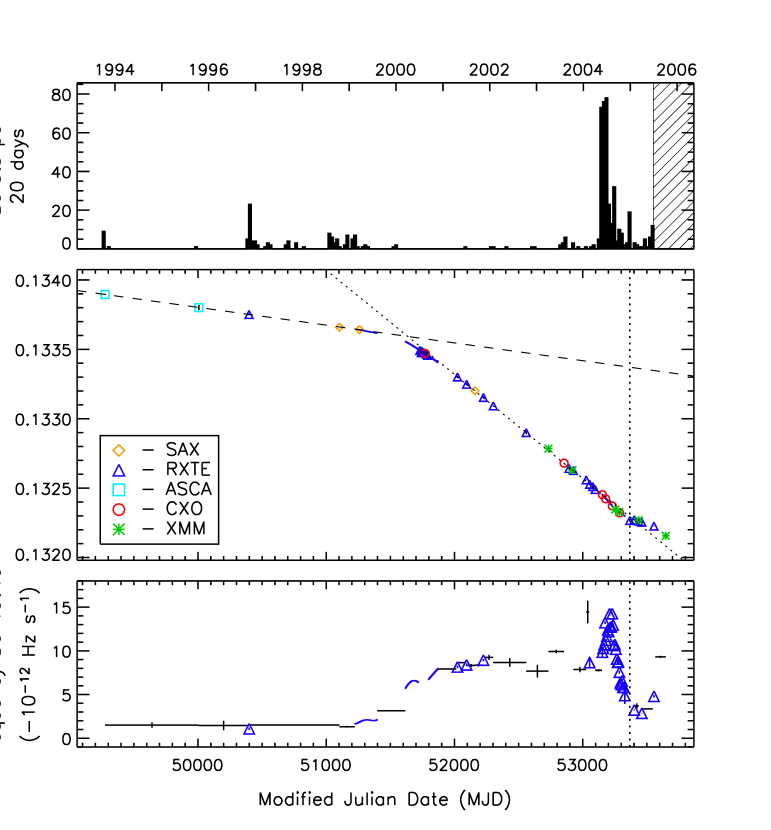
Figure 1: Pulse frequency and frequency derivative history of SGR 1806$-$20 between 1993 and 2005. Top – Burst rate history (through 2004 October) as seen with instruments within the Inter-Planetary Network. The time of the giant flare is indicated in subsequent panels by a vertical black dotted line. The burst rate data are complete through 2005 June. Middle – Pulse frequency history of the SGR as measured using an array of X-ray detectors (see insert legend). The dashed black line indicates a fit to frequency measurements between 1993 and 2000 January ($\dot{\nu}$ = $-1.48\times 10^{-12}$ Hz s^-1). The diagonal dotted black line indicates a fit to frequency measurements between 2001 January and 2004 April ($\dot{\nu}$ = $-8.69\times 10^{-12}$ Hz s^-1). Bottom – Pulse frequency derivative history of the SGR. Blue triangles indicate instantaneous frequency derivative measurements made with the RXTE PCA. Solid blue lines indicate continuous frequency derivative measurements from high-order ($>$3) polynomial fits to long stretches of phase-connected PCA observations. Black lines indicate average frequency derivative values between widely spaced frequency measurements. See text for details.

Over the last 12 years, SGR 1806$-$20 has undergone two epochs of relatively steady spin down, but at very different rates. Between 1993 and 2000 January, the average spin-down rate was $-1.48\times 10^{-12}$ Hz s^-1, or $\sim$6 times smaller than between 2001 January and 2004 April ($-8.69\times 10^{-12}$ Hz s^-1). The dramatic change in spin-down rate that began in 1999 and lasted $\sim$2 years, occurred without any spectacular increase in burst activity, change in persistent flux, pulse profile profile change, etc..

Only during the months leading up to the giant flare did we begin to observe large-amplitude, short-lived deviations from steady spin down (Figure 2). However, the frequency measurements between 2001 January and 2004 April were too sparse to detect similar frequency derivative changes. The spin-down rate of SGR 1806$-$20 steadily dropped between 2004 August and November. After 2004 November 22, RXTE observations were suspended due to Sun-angle constraints. Note that the spin-down rate began dropping well before the giant flare on 2004 December 27 (MJD 53366). When we fit the frequency derivative measurements between MJD 53150 and 53300 to a quadratic, we measure a centroid of MJD 53209$\pm$1. Thus, the torque on the star reached a maximum $\sim$5 months prior to the giant flare.

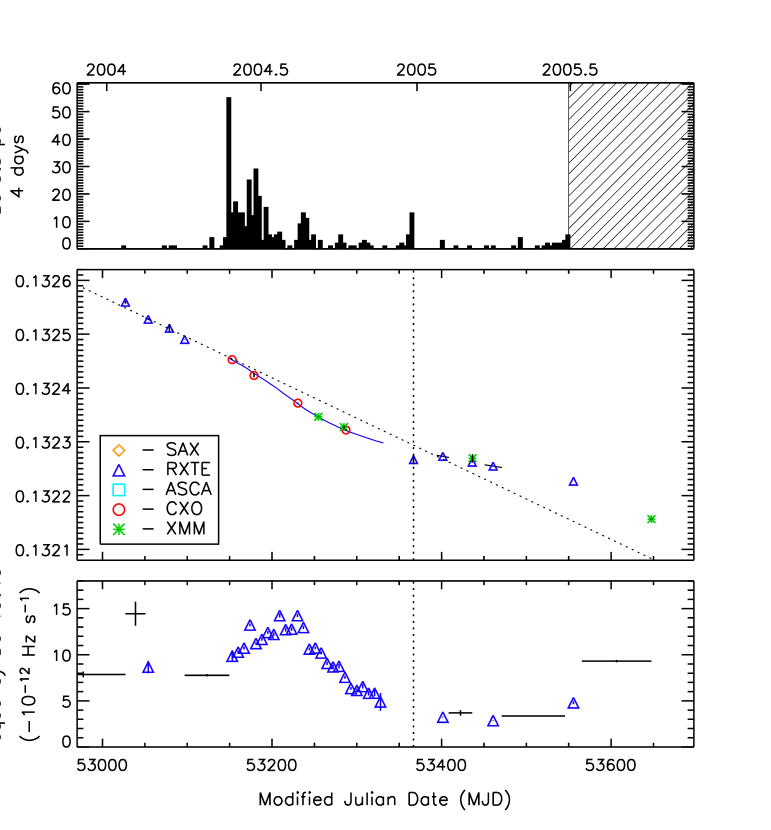
Figure 2: Pulse frequency and frequency derivative history of SGR 1806$-$20 during 2004 and 2005. Top – Burst rate history (through 2004 October) as seen with instruments within the Inter-Planetary Network. The time of the giant flare is indicated in subsequent panels by a vertical dotted line. The burst rate data are complete through 2005 June. Middle – Pulse frequency history of the SGR as measured using an array of X-ray detectors (see insert legend). The dotted black line indicates a fit to frequency measurements between 2001 January and 2004 April ($\dot{\nu}$ = $-8.69\times 10^{-12}$ Hz s^-1). The solid blue line indicates the frequency evolution measured by the quadratic spline fit to the RXTE observations during this interval. Bottom – Pulse frequency derivative history of the SGR. Blue triangles indicate instantaneous frequency derivative measurements made with the RXTE PCA. Black lines indicate average values between widely spaced frequency measurements. See text for details.

There was no measurable discrete jump in frequency of either sign at the time of the flare. Extrapolating the last pre-flare and first post-flare ephemerides to the time of the flare, we find an insignificant difference between the two predicted frequencies of 3.1$\pm$2.0 $\times$ 10^-7 Hz where the forward extrapolation yielded the larger expected frequency. The error reported here reflects the statistical error only and not the (dominant) systematic error caused by the strong timing noise of SGR 1806$-$20. Both extrapolations are consistent with the relatively imprecise pulse frequency measured during the tail of the flare itself (Woods et al. 2005). During the tail of the flare, the pulse profile changed dramatically and significantly biased the pulse frequency measurement. Thus, the formal 3$\sigma$ upper limit on the size of a hypothetical flare-induced frequency jump is $|\frac{\Delta\nu}{\nu}|<5\times 10^{-6}$. This limit is more than one order of magnitude smaller than the frequency jump inferred for SGR 1900$+$14 ($\frac{\Delta\nu}{\nu}\approx-1\times 10^{-4}$) at the time of the August 27 flare (Woods et al. 2001). We caution that the necessary frequency extrapolations employed here are susceptible to significant errors if the spin down rate of SGR 1806$-$20 changed significantly during the 63 day gap in observations. Moreover, this particular SGR has been known for some time to exhibit strong timing noise (Woods et al. 2000). However, the spin down changes would have had to have been large in amplitude, short-lived in duration, and precisely constructed in order to counter-balance a frequency jump as large as $|\frac{\Delta\nu}{\nu}|\approx 1\times 10^{-4}$ and still give the appearance of no flare-induced frequency jump when viewed with the existing data. We consider this scenario highly improbable.

The pre-flare reduction in torque continued following the giant flare, gradually approaching the pre-2000 spin-down rate 4$-$6 months following the flare. However, this trend quickly reversed itself one year after the flare and the most recent spin-down rate is equal to the nominal rate seen between 2001 and 2004.

4 Pulse Morphology Changes

4.1 Temporal Evolution

Göğüş et al. (2002) investigated the pulse profile evolution of SGR 1806$-$20 between 1996 and 2001 using RXTE monitoring data. During the first couple weeks of the 1996 outburst, the 2$-$10 keV pulse profile of SGR 1806$-$20 consisted of a broad, double-peaked pulse. Due to Sun-angle pointing constraints for RXTE, the source was not observed before the end of the outburst. At some point between 1996 November and 1999 February, the next time this SGR was observed, the pulse profile of the SGR simplified to a single, narrow pulse. We note that the majority of the burst energy emitted during the 1996 outburst followed the sequence of PCA observations used to construct this pulse profile. Thus, it is not known whether the pulse shape change happened suddenly during the intense portions of the 1996 outburst, or if the change was more gradual on a timescale of months to years. Between 1999 and 2001, the pulse morphology showed little or no change.

Folding our PCA data on the pulse ephemerides given in the last section, we have extended the 2$-$10 keV pulse morphology history of SGR 1806$-$20 through 2005 April (Figure 3). Very little additional change in pulse shape was observed between 2001 and the months leading up to the giant flare. However, we note that there was one interval in 2003 where the profile was temporarily more complex. In the months preceding the flare, the source brightened (see §5) and the 2$-$10 keV pulse shape became somewhat more jagged, yet retained the same overall pulse envelope. The most profound change occurred following the giant flare of 2004 December 27 when the pulse shape exhibited two clear peaks in 2005 January/February, markedly different that the pre-flare pulse shape over the same energy range. However, this change appears to have been short-lived as the pulse profile continued to evolve to a broad, flat-topped peak in 2005 March/April.

Figure 3: Pulse morphology evolution of SGR 1806$-$20 as seen with the RXTE PCA between 1996 and 2005. All pulse profiles shown are 2$-$10 keV and are repeated once for clarity (0$-$2 cycles). Note the change in pulse shape across the giant flare from 2004 to 2005. See text for details.

Qualitatively similar pulse shape evolution was observed during the tail of the giant flare from SGR 1806$-$20, albeit at much higher photon energies and luminosities (e.g. Palmer et al. 2005). Specifically, the complexity of the pulse profile defined as the power contained in the higher harmonics relative to the fundamental frequency increased during the tail of the flare. Although the direction of the pulse shape change in the quiescent emission was the same (i.e. the persistent pulse shape became more complex following the flare), the pulse shape of the persistent emission, even now, is much simpler than the pulse shape at any time during the tail of the flare.

Flare-induced pulse shape changes have also been seen in SGR 1900$+$14 following the 1998 August 27 giant flare (Woods et al. 2001; Göğüş et al. 2002). In the case of SGR 1900$+$14, the quiescent pulse profile suddenly changed from a complex multi-peaked morphology before the giant flare to a nearly sinusoidal single peak after the event. Similarly, the pulse profile during the 5-minute long flare tail evolved from a complex pulse pattern to a simpler, nearly sinusoidal pulse shape toward the end. Although both flares resulted in sustained changes in the quiescent pulse shape, it is important to note that the direction of the change was different for each flare. The SGR 1900$+$14 pulse profile simplified whereas the SGR 1806$-$20 pulse profile became more complex.

4.2 Energy Dependence

Göğüş et al. (2002) noted that there was no significant energy dependence of the pulse profile of SGR 1806$-$20 over the energy range 2$-$30 keV during PCA observations between 1996 and 2000. The pulse profile during 2001 showed signs of greater complexity at high energies (20$-$30 keV), although the signal-to-noise ratio for that data set was poor. Similarly, the 2002 and 2003 data sets did not provide enough counts at energies above $\sim$7 keV to construct meaningful pulse profiles. Here, we investigate the energy dependence of the SGR 1806$-$20 pulse profile at epochs leading up to and following the giant flare when the source was brightest.

Figure 4: Pulse profile evolution of SGR 1806$-$20 in time and energy as seen with the RXTE PCA in the months prior to and following the giant flare. Time increases from left to right and energy increases from top to bottom. All pulse profiles shown repeated once for clarity (0$-$2 cycles). See text for details.

Using the PCA data, we constructed three sets of pulse profiles over three separate energy ranges between 2 and 40 keV (Figure 4). Approximately six months before the flare, the pulse profile below 15 keV was fairly simple whereas the high energy profile (15$-$40 keV) showed two clear peaks per rotation cycle. The higher amplitude peak was correlated with the much broader low-energy pulse maximum and the secondary peak was $\sim$0.5 cycle later in phase – approximately aligned with pulse minimum at low energies. At two months prior to the flare, the pulse profile at intermediate energies (7$-$15 keV) became two-peaked and the relative amplitudes of the two peaks at high energies switched. One month following the giant flare, the pulse profile was very different showing multiple peaks at all energies. The dominant peak at high energies post-flare was seen as a narrow peak at intermediate and low energies. Although the most profound pulse shape changes took place across the flare, it is clear that the pulse profile of SGR 1806$-$20 was evolving in both time and energy during the year leading up to the flare.

4.3 Pulsed Fraction

The pulsed fraction of SGR 1806$-$20 is important in that it enables us to estimate the total flux of the SGR when we do not know the precise level of the background in the detector. This is relevant for all RXTE PCA observations which constitute the vast majority of our data set. We estimate the total (phase-averaged) flux of the SGR by taking the root mean square (r.m.s.) pulsed flux and dividing by the r.m.s. pulsed fraction. Here, we adopt the r.m.s. definition of the pulsed fraction given in Woods et al. (2004a). The pulsed flux is given by

$$F_{RMS}=\sqrt{\sum_{k=1}^{4}\frac{\alpha_{k}^{2}+\beta_{k}^{2}-(\sigma_{\alpha_{k}}^{2}+\sigma_{\beta_{k}}^{2})}{2}},$$ (1)

where

$$\alpha_{k}=\frac{2}{N}\sum_{i=1}^{N}r_{i}\cos{2\pi\phi_{i}{k}}, \displaystyle\beta_{k}=\frac{2}{N}\sum_{i=1}^{N}r_{i}\sin{2\pi\phi_{i}{k}},$$

$$\sigma_{\alpha_{k}}^{2}=\frac{4}{N^{2}}\sum_{i=1}^{N}\sigma^{2}_{r_{i}}\cos^{2}{2\pi\phi_{i}{k}}, \displaystyle\sigma_{\beta_{k}}^{2}=\frac{4}{N^{2}}\sum_{i=1}^{N}\sigma^{2}_{r_{i}}\sin^{2}{2\pi\phi_{i}{k}}.$$

Here, $F_{RMS}$ is the pulsed flux, $F_{RMS}/\bar{F}$ is the pulsed fraction where $\bar{F}$ is the phase-averaged flux, $k$ refers to the harmonic number, $i$ refers to the phase bin, $N$ is the total number of phase bins, $\phi_{i}$ is the phase, $r_{i}$ is the count rate in the $i^{\rm th}$ phase bin, and $\sigma_{x_{i}}$ is the uncertainty in the count rate of the $i^{\rm th}$ phase bin. Note that the pulsed fractions reported here may sometimes differ from measurements reported in the literature by other authors using the same data sets. These differences are due mostly to differences in the definition of pulsed fraction.

When measuring the rms pulsed fraction, we used only data taken from X-ray imaging telescopes where the background could be accurately measured. For consistency, we chose to measure the pulsed fraction over the energy range 2$-$10 keV. For all observations, we extracted a source and background event list for the given energy range, folded the source events on the measured pulse period, subtracted the background count rate, and measured the rms pulsed fraction using the sum of the first 4 harmonics. The measured pulsed fractions are plotted in Figure 6. Prior to the giant flare, all pulsed fractions of SGR 1806$-$20 are consistent with being constant at $\sim$7%. Following the giant flare there is a significant drop to 2.5$\pm$0.8% during the 2005 Chandra observation (Rea et al. 2005). Subsequent XMM-Newton observations (Mereghetti et al. 2005) show a similarly low pulsed fraction, although more recent observations show the pulsed fraction recovering to its pre-flare level (Rea et al. 2005b). We discuss the implications the changing pulsed fraction has on our PCA pulsed flux normalization factor in §5.4.

5 X-ray Spectroscopy

Up until recently, X-ray spectroscopic studies of the persistent, phase-averaged emission from SGR 1806$-$20 showed that the energy spectrum could be modeled with a simple absorbed power-law (Sonobe et al. 1994; Mereghetti et al. 2000). Broad-band spectroscopy of the persistent emission has shown that this non-thermal component extends up to at least 100 keV without signs of rolling over (Mereghetti et al. 2005b; Molkov et al. 2005). In the era of high-throughput soft X-ray telescopes such as Chandra and XMM-Newton, we are now able to more precisely model the X-ray spectrum and identify deviations from the simple power-law parameterization.

In general, magnetar candidates (i.e. SGRs and AXPs) have energy spectra that are well modeled by the sum of a blackbody and a power-law. From Chandra observations in 2004, we identified the long sought after blackbody component in SGR 1806$-$20 (Woods et al. 2004b). Using XMM-Newton observations, Mereghetti et al. (2005a) also identified a thermal component in the X-ray spectrum, however, they measured a much higher temperature. Here, we present our analysis of the six Chandra observations of SGR 1806$-$20, place these results in context with the full spectral history of this SGR, and address the apparent discrepancy between the Chandra and XMM-Newton blackbody temperatures.

5.1 Chandra Spectral Analysis

All six Chandra observations of SGR 1806$-$20 were performed in CC mode having one spatial dimension. We extracted source spectra from within a 10 pixel ($5^{\prime\prime}$) region centered on the peak of the one-dimentional image. The background spectra were extracted from two 40 pixel ($20^{\prime\prime}$) regions on either side of the SGR whose centers were offset from the source centroid by 40 pixels. As described in the section on Chandra timing analysis (§3.1), bursts were first removed from the event lists before compiling the energy spectra. The source spectra were rebinned to ensure at least 25 counts were contained within each energy bin. The effective area files and response matrices were constructed using the CIAO 3.2.1 procedures mkrmf and mkarf, respectively. The calibration database used to create these files was version 3.0.1.

Using XSPEC v11.3, we fit each spectrum individually to a power-law (PL) model and the sum of a blackbody plus a power law (BB$+$PL). A narrow feature at 1.7 keV was seen in the residuals of all fits. This feature is almost certainly instrumental in origin due to inaccuracies of the instrumental response. Artificial narrow features between 1.5 and 2.0 keV are commonly observed in Chandra CC-mode energy spectra of bright point sources. For this reason, we have limited our fit range to energy channels where the response is best calibrated between 0.5$-$1.6 and 2.0$-$10.0 keV.

For all six observations, the $\chi^{2}$ improved when the blackbody component was included in the fit. The improvement in $\chi^{2}$ varied from 7 to 19 with an average change in $\chi^{2}$ of 14. The significance of the thermal component in the observed spectrum was, on average, marginal for any given data set. To more sensitively probe our model comparison, we fit all six spectra simultaneously, forcing only the column density to be linked for all spectra. Comparing the PL and BB$+$PL model fits, we found that the total $\chi^{2}$ dropped by 93 with the addition of the 12 free blackbody parameters in the simultaneous fit. The F-test between these two models yielded a probability of 4 $\times$ 10^-14, indicating that the BB$+$PL model was strongly favored over the simple PL model. All fit parameters for both the PL and BB$+$PL models are listed in Table 5.

Table 5: Measured spectral parameters of SGR 1806$-$20 from Chandra observations.

Observation	Modela	NH	$kT$	$\Gamma$	Flux	Unabs. Flux
		(1022 cm-2)	(keV)		(10-11 ergs cm-2 s-1)b
CXO1	PL	7.1(3)	…	1.89(8)	1.21	1.95
	BB$+$PL	8.0(8)	0.48(9)	1.57(23)	1.27	2.20
	PL(s)	7.88(7)	…	2.09(4)	1.17	2.05
	BB$+$PL(s)	8.78(3)	0.41(4)	1.69(14)	1.26	2.39
	BB$+$PL(us)	7.19(12)	0.57(5)	1.40(20)	1.28	2.05
CXO2	PL	8.1(2)	…	1.94(5)	1.88	3.19
	BB$+$PL	8.6(5)	0.49(8)	1.70(14)	1.94	3.43
	PL(s)	7.88(7)	…	1.89(3)	1.89	3.16
	BB$+$PL(s)	8.78(3)	0.45(4)	1.76(10)	1.93	3.50
	BB$+$PL(us)	7.19(12)	0.75(3)	1.14(17)	1.98	3.06
CXO3	PL	7.7(3)	…	1.77(7)	2.09	3.38
	BB$+$PL	8.5(8)	0.49(9)	1.47(20)	2.18	3.76
	PL(s)	7.88(7)	…	1.81(4)	2.08	3.41
	BB$+$PL(s)	8.78(3)	0.47(5)	1.50(14)	2.18	3.86
	BB$+$PL(us)	7.19(12)	0.71(4)	0.98(24)	2.23	3.39
CXO4	PL	7.7(2)	…	1.64(5)	2.39	3.75
	BB$+$PL	7.8(5)	0.59(14)	1.39(19)	2.45	3.87
	PL(s)	7.88(7)	…	1.69(3)	2.37	3.79
	BB$+$PL(s)	8.78(3)	0.43(4)	1.56(9)	2.42	4.20
	BB$+$PL(us)	7.19(12)	0.75(5)	1.14(16)	2.48	3.70
CXO5	PL	8.1(2)	…	1.85(5)	2.47	4.13
	BB$+$PL	9.0(6)	0.44(6)	1.69(12)	2.53	4.61
	PL(s)	7.88(7)	…	1.79(3)	2.49	4.08
	BB$+$PL(s)	8.78(3)	0.46(5)	1.67(10)	2.53	4.50
	BB$+$PL(us)	7.19(12)	0.78(4)	1.11(17)	2.59	3.94
CXO6	PL	8.0(2)	…	2.06(6)	2.05	3.57
	BB$+$PL	10.2(8)	0.33(3)	2.09(12)	2.07	4.74
	PL(s)	7.88(7)	…	2.04(4)	2.06	3.55
	BB$+$PL(s)	8.78(3)	0.41(4)	1.91(10)	2.10	3.98
	BB$+$PL(us)	7.19(12)	0.70(4)	1.37(18)	2.16	3.43

^a PL = Power law; BB$+$PL = Blackbody plus power law; (s) indicates a simultaneous fit with the column density linked between all Chandra observations; (us) indicates a universal simultaneous fit with the column density linked between all observations (Chandra, XMM-Newton, BeppoSAX and ASCA).
^b Integrated over the energy range 2$-$10 keV.

The average blackbody temperature of SGR 1806$-$20 measured using the Chandra data is 0.44 keV, very near the measured temperature of SGR 1900$+$14 as well as most other magnetar candidates (e.g. Woods & Thompson 2006). However, we find that the temperature we measure is systematically smaller than the temperature measured using XMM-Newton data (Mereghetti et al. 2005a), even when the Chandra and XMM-Newton observations are nearly simultaneous. For example, XMM-Newton observed SGR 1806$-$20 on 2004 October 6 (ObsD in Mereghetti et al.), just 3 days before CXO5 with Chandra. For this XMM-Newton observation, Mereghetti et al. (2005) measured a temperature of 0.77$\pm$0.15 keV, a photon index of $-$1.2$\pm$0.2, and a column density of 6.5$\pm$0.6 $\times$ 10²² cm^-2, all significantly different than the parameters derived from the CXO5 Chandra data (see Table 5). In an effort to resolve this discrepancy, we analyzed this observation and all other publicly available XMM-Newton observations of SGR 1806$-$20.

5.2 Comparison to XMM-Newton Results

There have been six observations of SGR 1806$-$20 carried out with XMM-Newton between 2003 April and 2005 October. The times of these observations and their approximate exposure times are listed in Table 6. An analysis of the four observations through 2004 October has been presented in Mereghetti et al. (2005a). The post-flare XMM-Newton observations of SGR 1806$-$20 were presented by Tiengo et al. (2005) and Rea et al. (2005b). Here, we present our analysis of PN energy spectra of the persistent X-ray emission recorded during all six XMM-Newton observations.

Table 6: XMM-Newton observation log for SGR 1806$-$20 between 2003 April and 2005 October.

Name	XMM-Newton	Date	PN Exposure
	Observation ID		(ks)
XMM1	0148210101	2003 Apr 03	55.5
XMM2	0148210401	2003 Oct 07	22.4
XMM3	0205350101	2004 Sep 06	51.9
XMM4	0164561101	2004 Oct 06	18.9
XMM5	0164561301	2005 Mar 07	24.9
XMM6	0164561401	2005 Oct 04	33.0

During the first two XMM-Newton observations of SGR 1806$-$20 in 2003, the PN camera was operated in Full Frame (FF) mode. The four subsequent observations have been operated in Small Window (SW) mode to better study SGR burst emissions. The SW mode has finer time resolution and can tolerate a greater dynamic flux range than FF mode. In all observations, the medium thickness filter was used. Starting from the Observation Data Files, we processed the PN data using the script epchain provided in the XMM Science Analysis Software (XMMSAS) v6.5.0. Next, we constructed a light curve of the central PN CCD, excluding the bright central source, and identified times of high background. We chose a threshold of 2 times the nominal 0.5$-$10.0 keV background to define regions of high background. Accordingly, we filtered out 0$-$40% of the total exposure from each data set before subsequent analysis. Finally, we constructed light curves of SGR 1806$-$20 at 1 s time resolution to identify bursts. Using custom software, we filtered out several tens of SGR bursts from the event lists.

Using our filtered event lists, we extracted source spectra from $37.5^{\prime\prime}$ (750 pixel) radii circular regions centered on the SGR and background spectra from $\sim 67^{\prime\prime}$ radii circular regions from the same CCD. We followed standard XMMSAS recipes in grade selection (pattern $<$4) and generation of effective area files and response matrices.

Using XSPEC v11.3, we fit the individual XMM-Newton spectra over the energy range 0.5$-$10.0 keV to both the PL and BB$+$PL models. Similar to the Chandra spectral results, we measured small changes in $\chi^{2}$ for 4 individual spectral fits ($\Delta\chi^{2}=9-18$). The two exceptions were observations XMM3 and XMM5 which yielded a reduction in $\chi^{2}$ of 27 and 37, respectively, between the PL and BB$+$PL models. The improvement in $\chi^{2}$ for these two data sets was significant. The combined simultaneous fit to all XMM-Newton energy spectra indicated that the inclusion of the blackbody component was again very significant (F-test probability $\approx 10^{-14}$). The fit parameters for all spectral fits are given in Table 7. We note that the fit parameters we measure are mostly consistent with the results of Mereghetti et al. (2005a), Tiengo et al. (2005), and Rea et al. (2005b). On average, we measure slightly higher column densities and steeper photon indices than Mereghetti et al.. These subtle differences could be caused by choices of energy fit range and/or binning – for example.

Table 7: Measured spectral parameters of SGR 1806$-$20 from XMM-Newton observations.

Observation	Modela	NH	$kT$	$\Gamma$	Flux	Unabs. Flux
		(1022 cm-2)	(keV)		(10-11 ergs cm-2 s-1)b
XMM1	PL	6.6(3)	…	1.63(6)	1.08	1.61
	BB$+$PL	7.2(7)	0.54(12)	1.41(15)	1.09	1.72
	PL(s)	7.12(6)	…	1.73(4)	1.07	1.67
	BB$+$PL(s)	6.63(2)	0.65(7)	1.29(15)	1.10	1.64
	BB$+$PL(us)	7.19(12)	0.54(6)	1.41(12)	1.09	1.71
XMM2	PL	6.7(2)	…	1.64(5)	1.20	1.80
	BB$+$PL	6.8(5)	0.66(12)	1.32(18)	1.21	1.84
	PL(s)	7.12(6)	…	1.72(3)	1.19	1.85
	BB$+$PL(s)	6.63(2)	0.72(5)	1.16(14)	1.22	1.81
	BB$+$PL(us)	7.19(12)	0.61(5)	1.32(11)	1.21	1.90
XMM3	PL	7.2(1)	…	1.56(2)	2.48	3.75
	BB$+$PL	6.7(3)	0.85(7)	1.14(14)	2.50	3.63
	PL(s)	7.12(6)	…	1.55(2)	2.48	3.74
	BB$+$PL(s)	6.63(2)	0.86(5)	1.12(10)	2.50	3.62
	BB$+$PL(us)	7.19(12)	0.71(5)	1.34(7)	2.50	3.78
XMM4	PL	7.3(2)	…	1.69(4)	2.44	3.80
	BB$+$PL	6.7(5)	0.84(10)	1.21(24)	2.46	3.64
	PL(s)	7.12(6)	…	1.65(2)	2.44	3.75
	BB$+$PL(s)	6.63(2)	0.85(5)	1.18(13)	2.46	3.62
	BB$+$PL(us)	7.19(12)	0.72(5)	1.42(10)	2.45	3.78
XMM5	PL	7.1(2)	…	1.72(4)	1.95	3.03
	BB$+$PL	6.0(4)	0.91(6)	0.65(36)	1.99	2.80
	PL(s)	7.12(6)	…	1.72(3)	1.95	3.04
	BB$+$PL(s)	6.63(2)	0.79(4)	1.05(16)	1.98	2.95
	BB$+$PL(us)	7.19(12)	0.70(4)	1.27(12)	1.98	3.09
XMM6	PL	7.2(2)	…	1.83(4)	1.30	2.08
	BB$+$PL	6.6(4)	0.77(7)	1.19(22)	1.32	2.00
	PL(s)	7.12(6)	…	1.81(3)	1.54	2.07
	BB$+$PL(s)	6.63(2)	0.76(4)	1.28(13)	1.32	2.00
	BB$+$PL(us)	7.19(12)	0.65(4)	1.49(10)	1.32	2.10

^a PL = Power law; BB$+$PL = Blackbody plus power law; (s) indicates simultaneous fit with the column density linked between all XMM-Newton observations; (us) indicates a universal simultaneous fit with the column density linked between all observations (Chandra, XMM-Newton, BeppoSAX and ASCA).
^b Integrated over the energy range 2$-$10 keV.

When plotted on the same scale, all XMM-Newton spectral measurements (including blackbody temperature) resulting from individual spectral fits are systematically offset from nearby Chandra measurements indicating a discrepancy between the two instruments. The consistent offset in individual spectral parameters suggests that the differences are instrumental and not due to intrinsic variability of the SGR.

In spite of the differences between the Chandra and XMM-Newton spectral parameters, our joint analysis of the two data sets allowed us to conclude that ($i$) the simple power-law model does not accurately represent the X-ray energy spectrum of SGR 1806$-$20 and ($ii$) the addition of a thermal component yields acceptable spectral fits. To further investigate the residual differences between the Chandra and XMM-Newton results, we attempted inter-instrument simultaneous fitting of all available SGR 1806$-$20 data sets.

5.3 Universal Simultaneous Fit

Prior to the 12 Chandra and XMM-Newton observations of SGR 1806$-$20 presented here, there were four BeppoSAX observations between 1998 and 2001 (Mereghetti et al. 2000) and two ASCA observations in 1993 (Sonobe et al. 1994) and 1995 suitable for spectral fitting. The ASCA GIS data were processed following standard analysis procedures outlined in the ASCA data analysis guide. Similarly, the BeppoSAX LECS and MECS data were processed using Xselect as directed in the BeppoSAX guide. As with the previous simultaneous fits, we forced the column density to be the same for all observations. Due to poorer signal-to-noise quality of the ASCA spectra, we fixed the blackbody temperature for these data sets equal to the mean of the four measured BeppoSAX temperatures. All other spectral parameters were free to vary in the fit. The measured values are listed in Tables 5, 7 and 8 in the rows labeled “us.”

Table 8: Measured spectral parameters of SGR 1806$-$20 from ASCA and BeppoSAX observations.

Observation	Modela	NH	$kT$	$\Gamma$	Flux	Unabs. Flux
		(1022 cm-2)	(keV)		(10-11 ergs cm-2 s-1)b
ASCA1	BB$+$PL(us)	7.19(12)	0.476	1.44(13)	0.91	1.70
ASCA2	BB$+$PL(us)	7.19(12)	0.476	1.67(15)	0.70	1.36
SAX1	BB$+$PL(us)	7.19(12)	0.49(8)	1.75(22)	1.04	1.79
SAX2	BB$+$PL(us)	7.19(12)	0.44(10)	1.95(13)	1.06	1.83
SAX3	BB$+$PL(us)	7.19(12)	0.47(7)	1.77(20)	0.99	1.73
SAX4	BB$+$PL(us)	7.19(12)	0.50(6)	1.66(16)	1.15	1.96

^a BB$+$PL = Blackbody plus power law; (us) indicates a universal simultaneous fit with the column density linked between all observations (Chandra, XMM-Newton, BeppoSAX and ASCA).
^b Integrated over the energy range 2$-$10 keV.

Simultaneously fitting all available SGR 1806$-$20 data with a single column density fitted for all observations significantly reduced the discrepancy between our Chandra results and the XMM-Newton results. For the universal simultaneous fit, we obtain a statistically acceptable $\chi^{2}$ of 8379 for 8421 degrees of freedom. We now find very good agreement between the measured blackbody temperatures, power-law photon indices, and X-ray fluxes. For example, consider the near simultaneous Chandra and XMM-Newton observations in 2004 October (CXO5 and XMM4). For the independent spectral fits, the measured blackbody temperatures differed by 3.5$\sigma$, the photon index by 1.8$\sigma$, and unabsorbed flux by 26%. When we linked the column density in the universal simultaneous fit, these differences were reduced to less than 1.6$\sigma$ for all parameters (see Table 5 and 7 for additional examples).

The improved agreement between the Chandra and XMM-Newton results for the simultaneous fit with a linked column density suggests that the instrumental “discrepancy” we noted originally is likely due to strong coupling of the spectral parameters in combination with slight differences in the instrumental response functions of the two instruments. The cross-correlation between the blackbody parameters and the column density is particularly strong and that is where we observed the largest disparity. By forcing the column density to be the same for all data sets, we effectively reduced the covariance between these parameters.

5.4 Spectral History

Combining our Chandra, XMM-Newton, BeppoSAX, and ASCA spectral results on SGR 1806$-$20, we constructed a comprehensive spectral history of the SGR from 1993 to 2005 (Figure 5). Shown are the spectral parameters derived from the universal simultaneous spectral fit described in the previous section. Note that the blackbody temperature was fixed for the ASCA spectra to the average of the four BeppoSAX temperatures. As can be seen in this figure, the unabsorbed flux showed very little variability between 1993 and 2002 before increasing by more than a factor 2 during the 2004 burst active episode. Correlated with the peak in flux in 2004 was a maximum in blackbody temperature and minimum in photon index. The increased spectral hardness was evidenced in both the thermal and non-thermal components of the spectrum. Interestingly, each began to show changes in early 2003 – more than one year prior to the giant flare (vertical dotted line).

As with the torque on the star, the peaks (valley) in these three spectral parameters appear to precede the flare itself. We fitted the blackbody temperature and photon index measurements between MJD 52700 and 53700 to a quadradic and measured centroids of 53280$\pm$40 and 53160$\pm$60, respectively. The X-ray flux was more peaked, so we limited our fit range to MJD 53000 to 53500 and measured a centroid of 53296$\pm$8. All three cenroid values precede the giant flare (MJD 53366) by several months. However, our data coverage for spectral measurements is admittedly much more sparse than our frequency derivative measurements and these maxima are relatively broad.

Figure 5: Spectral history of SGR 1806$-$20 from 1993 to 2005 using the blackbody plus power-law model simultaneously fit to all data sets. The measured column density for this fit was 7.19$\pm$0.12 cm^-2. From top to bottom, IPN burst rate history, blackbody temperature, photon index, and unabsorbed flux. The time of the giant flare is indicated by a vertical dotted line. The burst rate data are complete through 2005 June. Horizontal dashed lines indicate the average value for the given parameter for measurements before 2002. See text for details.

To further investigate the flux variability of SGR 1806$-$20, we included pulsed flux measurements of the SGR obtained using RXTE PCA data. Following the method described in Woods et al. (2001 and 2004) for SGR 1900$+$14 and 1E 2259$+$586, respectively, we folded individual segments of 2$-$10 keV PCA data to created high signal-to-noise pulse profiles. We computed the r.m.s. pulsed amplitude of each segment by summing the power of the first 4 harmonics according to equation 1. In Figure 6, we show the pulsed flux and phase-averaged unabsorbed flux values (also plotted in Figure 5). The far more numerous PCA pulsed fluxes provide a more comprehensive picture of the flux evolution of the SGR over the last decade. The pulsed flux axis (right) is referenced to the phase-averaged flux axis by calculating a scale factor between the two from PCA pulsed flux measurements in 1999 and a contemporaneous phase-averaged flux measurement from BeppoSAX. Assuming that the pulsed fraction of SGR 1806$-$20 remains constant (and perfect X-ray detector intercalibration), the PCA pulsed fluxes on this scale would exactly match all other phase-averaged fluxes. With the exception of the months leading up to and following the giant flare, there is generally good agreement between the two. The post-flare disparity is clearly due to the sudden drop in pulsed fraction (bottom panel). The pre-flare mismatch could be due to a change in the energy dependence of the pulsed fraction during the flux rise.

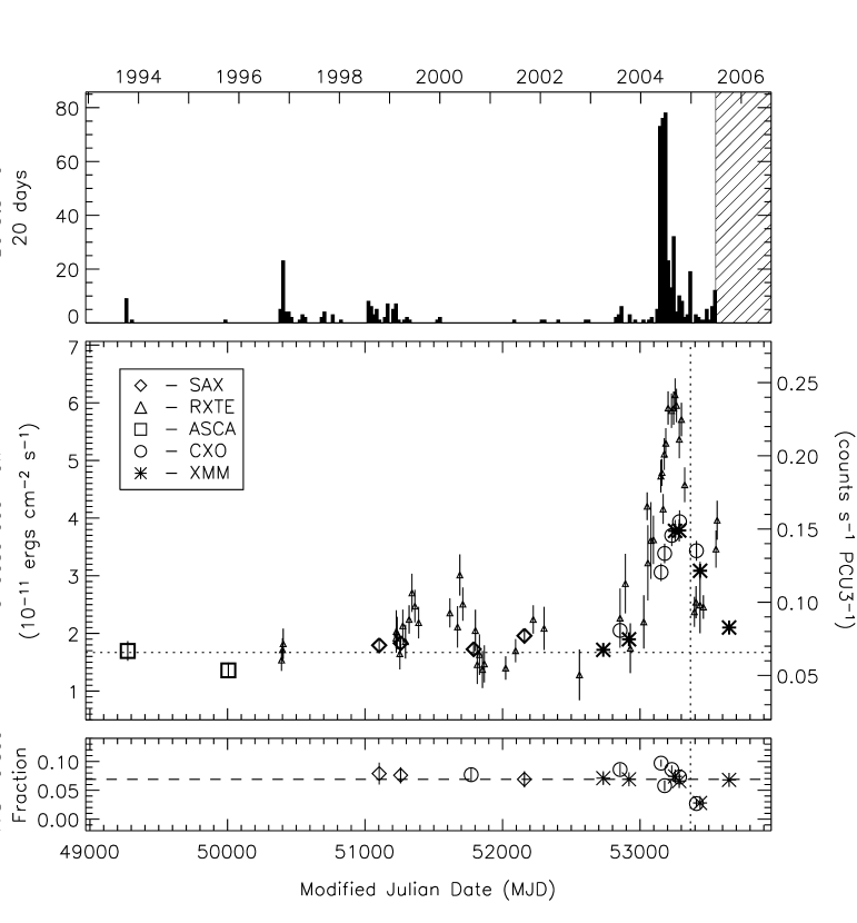
Figure 6: Persistent and pulsed flux history of SGR 1806$-$20 between 1993 and 2005. Top – Burst rate history (through 2004 October) as seen with instruments within the Inter-Planetary Network. The time of the giant flare is indicated in subsequent panels by a vertical dotted line. The burst rate data are complete through 2005 June. Middle – Persistent and pulsed flux history of the SGR (2$-$10 keV). Unabsorbed fluxes (left axis) measured using imaging X-ray telescopes such as ASCA, BeppoSAX, Chandra, and XMM-Newton. The pulsed fluxes (right axis) are measured using RXTE. The pulsed flux measurements are “normalized” to the phase-averaged flux level assuming a constant pulsed fraction of $\sim$7%. The horizontal dotted line indicates the pre-2000 average flux level using ASCA and SAX measurements. Solid curved lines indicate fits to a quadratic model for data between MJD 53000 and 53500. See text for details. Bottom – Pulsed fraction (2$-$10 keV) as measured using the imaging X-ray telescopes.

Low-level changes in the pulsed flux of SGR 1806$-$20 are evident between 1999 and 2003, although the largest magnitude changes in flux occurred during the time leading up to and following the giant flare. A close-up of the flux evolution during this epoch (Figure 7) shows that the flux rose on a timescale of months in the build-up to the flare. As with the torque, spectral hardness and phase-averaged flux, the pulsed flux peaks well before the flare itself on 2004 December 27. Fitting the pulsed flux data between MJD 53000 and 53500 to a quadratic, we find the centroid at MJD 53227$\pm$8, nearly 5 months prior to the flare.

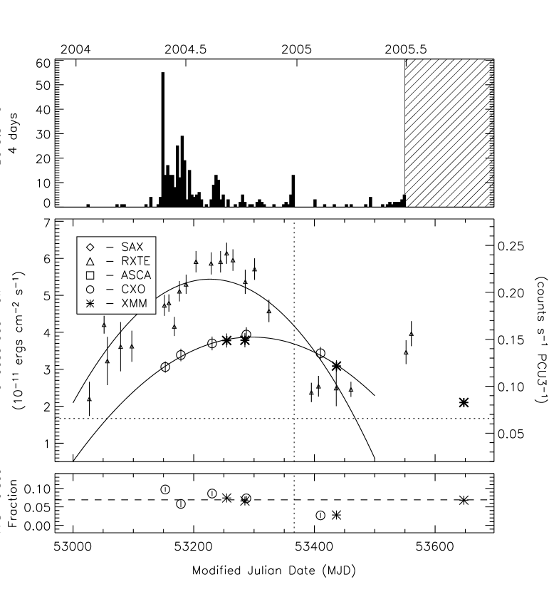
Figure 7: Persistent and pulsed flux history of SGR 1806$-$20 between 2004 and 2005. Top – Burst rate history (through 2004 October) as seen with instruments within the Inter-Planetary Network. The time of the giant flare is indicated in subsequent panels by a vertical dotted line. The burst rate data are complete through 2005 June. Middle – Persistent and pulsed flux history of the SGR (2$-$10 keV). Unabsorbed fluxes (left axis) measured using imaging X-ray telescopes such as Chandra and XMM-Newton. The pulsed fluxes (right axis) are measured using RXTE. The pulsed flux measurements are “normalized” to the phase-averaged flux level assuming a constant pulsed fraction of 7%. See text for details. Bottom – Pulsed fraction (2$-$10 keV) as measured using the imaging X-ray telescopes.

6 Discussion

Similar to outbursts in other magnetar candidates, the intense burst activity of SGR 1806$-$20 in 2004 was accompanied by changes in the persistent and pulsed emission properties of the source. Specifically, we observed a hardening of the X-ray spectrum, large amplitude increases in the pulsed and phase-averaged flux, strong variability in the spin-down rate, and significant changes in the pulse morphology. The connection between burst activity and the persistent emission of magnetar candidates has allowed us to place constraints on the magnetar model, and at times motivate refinements to the model. Below, we discuss how the changes we observed in the persistent X-ray emission of SGR 1806$-$20 during the 2004 outburst fit within the magnetar model.

Mereghetti et al. (2005a) reported a correlation between spectral hardness and spin-down rate (i.e. torque) of SGR 1806$-$20 for X-ray observations preceding the giant flare. They report a monotonic increase in spectral hardness from 1993 to 2004. Our analysis of the data is consistent with their conclusion that the energy spectrum hardens over the last decade, however, we find significant differences in the temporal evolution and consequently the hardness-torque correlation. With regard to the spectral evolution, our universal simultaneous fit shows that the X-ray spectrum does not begin to harden until at least 1999. In fact, the data do not show a clear hardening trend until 2003. From this period through mid-2005, the photon index steadily flattens with time and the blackbody temperature increases. Our RXTE monitoring observations of SGR 1806$-$20 show that the torque change, on the other hand, was relatively sudden in 2000 taking $\sim$1 year to transition to a new equilibrium state where the spin-down rate remained roughly constant until 2004. Only during this $\sim$4 year interval of steady, enhanced torque did the energy spectrum become harder. If, in fact, the two effects are correlated in SGR 1806$-$20, the torque change in year 2000 preceded the gradual hardening of the spectrum as opposed to a monotonic evolution of each parameter in lock-step with the other as suggested by Mereghetti et al..

Early in 2004, the torque on SGR 1806$-$20 began to increase again reaching a maximum $\sim$2 months after the peak in burst rate, but still several months before the flare epoch. Similarly, the energy spectrum peaked in hardness after the burst rate peak and before the flare epoch. The spectral hardness peak appears to be delayed relative to the torque maximum. As the torque underwent a rapid decline, the energy spectrum followed with a gradual softening. These trends continued through the flare epoch without deviating. Approximately three months after the flare, the torque reached a local minimum and has since recovered to the pre-flare level of 2001$-$2004. The spectral hardness, on the other hand, has continued to drop and is steadily approaching the pre-2000 spectral shape.

In summary, the correlation between torque and spectral hardness is not straightforward. There is evidence in favor of the torque change in year 2000 preceding, perhaps triggering a gradual hardening of the energy spectrum. However, the pre-flare drop in torque and its subsequent post-flare recovery resulted in a spectral softening, but no recovery (as of yet) in the spectral hardness. This may indicate some level of histeresis in the system.

A correlation between spectral hardness and torque is expected in the model of Thompson et al. (2002) for a magnetar with a twisted magnetosphere. It is hypothesized that a twist is imparted on the magnetosphere from below as residual magnetic field complexities within the interior of the star work their way to the surface and deform the crust in energetically favorable rotational motions. The subsequent twisting of external field lines caused by this motion amplifies the current along these field lines giving rise to enhanced magnetospheric scattering of X-rays from below, and in the case of open field lines, increased torque on the star. Within the context of this model, the delayed spectral response would indicate that the open field lines near the magnetic poles were first affected by the twist causing the sudden increase in torque. If only a small bundle of field lines were initially involved, the phase-averaged energy spectrum would not be significantly altered. Assuming the current along closed field lines gradually increased over the next several years, so would the isotropic scattering of X-rays, and, consequently, the spectral hardness.

The pulsed flux of SGR 1806$-$20 correlates with the torque in the months surrounding the giant flare. In Figure 8, we show the frequency derivative (i.e. torque) versus pulsed flux between MJD 53050 and 53610. The Spearman rank order correlation coefficient for this data set is 0.66 which would be expected assuming the null-hypothesis (i.e. no correlation) with a probability of 6 $\times$ 10^-4. The measurements leading up to the peak in torque on MJD 53209 are indicated by open diamonds and the post-peak measurements are indicated by filled circles. There is some evidence that the decline in torque is more rapid than the pulsed flux decline since the filled circles reside systematically higher than the open diamonds over the same range in frequency derivative. Within the model of Thompson et al. (2000, 2002), the current flowing along open field lines determines the spin-down rate of the neutron star. This correlation suggests that the pulsed emission of the SGR is shaped by these currents in the outer magnetosphere. We note that no such correlation was seen in the epoch surrounding the sudden torque change in 2000. It is not clear why this correlation exists only over certain time intervals.

Figure 8: Frequency derivative versus pulsed flux for SGR 1806$-$20 during the epoch surrounding the burst active episode in 2004$-$2005 (MJD 53050$-$53610). Open diamonds indicate measurements preceding the peak in torque on MJD 53209. Filled circles indicate measurements following this peak. See text for details.

Another consequence of crustal twisting would be an increase in burst activity since the bursts are believed to be triggered by crustal fractures and/or magnetospheric reconnection events. We find that the burst frequency reached a maximum shortly before the peak in spin-down rate in 2004. This delay of $\sim$2 months could reflect the time scale at which the twist propogates from the stellar surface, presumably where the bursts originate, out to the light cylinder where the torque on the star is influenced. Curiously, there is no sudden rise in burst activity at the time of the torque change in 2000.

Magnetospheric currents strongly influence the pulsed intensity and morphology of the persistent X-ray emission from magnetars (Thompson et al. 2002). Similar to the giant flare from SGR 1900$+$14, the December 27^th flare from SGR 1806$-$20 had a lasting impact upon the pulse morphology of the X-ray emission which has persisted for several months following the flare. The fact that the pulse profile of SGR 1806$-$20 became more complex following the flare while the SGR 1900$+$14 pulse profile simplified suggests that these current distributions can become more complex or simplify as a consequence of the flare. This observation in combination with the sustained phase-averaged flux following both flares supports the assertion made from flare energetics (e.g. Hurley et al. 2005) that the ultimate energy source for these flares is likely internal to the star as opposed to relaxation of external currents.

The spin frequency evolution of SGR 1806$-$20 leading up to and following the giant flare was significantly different than the spin behavior seen in SGR 1900$+$14 at the time of its flare. There was good circumstantial evidence to suggest that SGR 1900$+$14 underwent a sudden change in frequency of $\frac{\Delta\nu}{\nu}\approx-1\times 10^{-4}$ at the time of the 1998 August 27 giant flare (Woods et al. 2001). Extrapolation of the pre-flare and post-flare spin ephemerides showed a clear mismatch in frequency at the time of the flare (Woods et al. 1999) and the pulse phase during the flare did not agree with a backward extrapolation of the post-flare pulse ephemeris (Palmer 2002). However, this conclusion was not definitive due to uncertainty in the pre-flare pulse frequency of SGR 1900$+$14 and energy dependence of the pulse profile during the flare. Assuming the frequency change was genuine, Thompson et al. (2000) hypothesized that the drop in spin frequency of at the time of the giant flare could have been caused by a particle outflow during the flare. In fact, the transient radio nebula detected in SGR 1900$+$14 (Frail, Kulkarni & Bloom 1999) supports the assertion of a particle outflow. Assuming the outflow is restricted to a fraction $f$ of the surface, and accounting for the dependence of the outflows angular momentum on the latitude $\theta$, we find

$${\Delta\nu\over\nu}\simeq 1\times 10^{-4}\,\left({\Delta E\over 10^{44}~{}{\rm erg}}\right)^{1/2}\,\left({\Delta t\over 100~{}{\rm s}}\right)^{1/2}\,\,f^{1/2}\,\sin^{2}\theta\,\left({B_{\star}\over 10~{}B_{\rm QED}}\right)\,\left({V\over 0.2c}\right)^{-3/2}.$$ (2)

where $\Delta E$ is the total kinetic energy of the particles blown off the surface during the flare, $\Delta t$ is the time scale of the outflow, $B_{\star}$ is the surface field strength, and $V$ is the velocity of the outflowing particles. Thompson et al. approximated the particle outflow parameters and assumed isotropic emission to match the inferred frequency change.

The SGR 1806$-$20 flare was $\sim$2 orders of magnitude more luminous in $\gamma$-ray/X-ray emission (Palmer et al. 2005) and radio emission (Gaensler et al. 2005). Moreover, extensive observations of the radio nebula provided measurements of the ejected mass ($M\simeq 5\times 10^{24}$ g [Gelfand et al. 2005]), the total particle energy ($\Delta E$ $\simeq$ 3 $\times$ $10^{44}$ ergs [Gelfand et al. 2005]), and the initial outflow velocity ($V\simeq 0.7c$ [Taylor et al. 2005]). For a surface dipole magnetic field strength of $\sim$10¹⁵ G inferred from the pulse timing parameters, the expected $\frac{\Delta\nu}{\nu}$ for SGR 1806$-$20 was

$${\Delta\nu\over\nu}\simeq 5\times 10^{-5}\,\left({\Delta t\over 100~{}{\rm s}}\right)^{1/2}\,\,f^{1/2}\,\sin^{2}\theta.$$ (3)

An ejection of this much mass from the surface of the star without producing a change in $\frac{\Delta\nu}{\nu}>5\times 10^{-6}$ would require that the particle outflow proceeded rapidly ($\sim$1 s) and/or the mass was expelled along the spin axis of the star. The non-spherical outflow of the material (Taylor et al. 2005; Fender et al. 2006; Granot et al. 2006) suggests that one or both of these requirements were met.

One of the most obvious differences between the effects of the giant flares of SGR 1806$-$20 and SGR 1900$+$14 on the persistent X-ray emission is the relative timing of the observed changes. In SGR 1900$+$14, the giant flare preceded and almost certainly triggered a flux enhancement and pulse profile change. For SGR 1806$-$20, the spectrum, flux and pulse profile were already changing several months before the flare, although the most significant pulse morphology transition occurred during/after the flare. In SGR 1900$+$14, there was no detected change in torque preceding the flare whereas SGR 1806$-$20 showed dramatic changes months before the flare epoch. The one pre-flare phenomenon common to both SGRs was the onset of intense burst activity in the months preceding their respective flares. It appears that the presence of intense burst activity is a necessary, but not sufficient condition to predict giant flares. There are some counter-examples where intense burst activity did not result in a giant flare (e.g. SGR 1806$-$20 in 1984 and 1996), although there could be a burst-intensity threshold that must be met in order to trigger a flare. The burst rate from SGR 1806$-$20 in the months preceding the giant flare was higher and more energy was released than in previously recorded outbursts. With only two well-studied examples, it is difficult to draw any firm conclusions on magnetar behavior that is predictive of a giant flare. However, since all persistent emission parameters behaved differently in the years leading up to the flares produced by these two SGRs, it appears that the burst activity is the most promising metric to use.

Appendix: Pulse Cycle Count Fitting Technique

We present here a method for estimating the pulse cycle counts between pulse phase measurements, and for quanitifing the uniqueness of the cycle counts determined. This method is based on $\chi^{2}$ fits of a set of pulse phase and frequency measurements using a polynomial phase model. An upper threshold value for the fit statistic $\chi^{2}_{max}$ is choosen, and all combinations of integer cycle counts which result in minimum $\chi^{2}$ values below this threshold are found using a tree search. If the lowest value of minimum $\chi^{2}$ is sufficiently separated from the next-lowest value, then the the cycle counts associated with lowest value $\chi^{2}$ are uniquely determined. Otherwise the cycle counts are ambiguous, with several combinations of cycle counts being possible.

For a short enough span of measurements (assuming no glitch has occured) we can model pulse phases $\phi_{i}$ and frequencies $\nu_{i}$ measured at barycentric times $t_{i}$ as

$$\phi_{i} = \sum_{j=0}^{M}a_{j}(t_{i}-T_{0})^{j}+\sum_{k=0}^{N-1}h(t_{i}-\tau_{k})$$

$$\nu_{i} = \sum_{j=1}^{M}a_{j}j(t_{i}-T_{0})^{j-1}$$ (4)

were the $a_{j}$ are the coeffients of an $M^{\rm th}$ order polynomial in time, $T_{0}$ is the time origin of the polynomial, the $n_{k}$ are integer offsets correcting any cycle slips, which are applied at times $\tau_{k}$ which are taken to be between measurements, and $h(x)$ is the Heavyside function which is 0 for $x<0$ and 1 for $x>0$.

The $\chi^{2}$ of the fit with this model may be written as

$$\chi^{2}=\left|\left(\begin{array}[]{ccc}A&H&{\bf z}\\ \acute{A}&0&{\bf\acute{z}}\end{array}\right)\left(\begin{array}[]{r}{\bf a}\\ {\bf n}\\ -1\end{array}\right)\right|^{2}$$ (5)

where $A$, $\acute{A}$ and $H$ are arrays with elements

$$A_{ij}=(t_{i}-T_{0})^{j}/\sigma_{\phi_{i}},~{}~{}H_{ik}=h(t_{i}-\tau_{k})/\sigma_{\phi_{i}},~{}~{}\acute{A}_{ij}=j(t_{i}-T_{0})^{j-1}/\sigma_{\nu_{i}},$$ (6)

${\bf z}$ and ${\bf\acute{z}}$ are vectors with elements

$$z_{i}=\phi_{i}/\sigma_{\phi_{i}},~{}~{}\acute{z}_{i}=\nu_{i}/\sigma_{\nu_{i}},$$ (7)

${\bf a}$ is the vector of polynomial coefficients, and ${\bf n}$ is the vector of integer cycle slip offsets, with $\sigma_{\phi_{i}}$ and $\sigma_{\nu_{i}}$ being the phase and frequency errors.

We will assume that for fixed cycle counts this fit is overdetermined. Using Householder transformations (a sequence of reflections of the column vectors) we can transform the matrix in equation 5 into upper-triangular form. The $\chi^{2}$ of the fit then has the form

$$\chi^{2} = \left|\left(\begin{array}[]{ccc}Q&R&{\bf s}\\ 0&U&{\bf v}\\ 0&0&w\end{array}\right)\left(\begin{array}[]{r}{\bf a}\\ {\bf n}\\ -1\end{array}\right)\right|^{2}$$ (14)

$$= |Q{\bf a}+R{\bf n}-{\bf s}|^{2}+|U{\bf n}-{\bf v}|^{2}+w^{2}~{}~{}.$$ (15)

For a given set of cycle counts ${\bf n}$ the estimates for the polynomal coefficents are

$$\hat{\bf a}=Q^{-1}({\bf s}-R{\bf n})~{}~{}{\rm with}~{}~{}{\rm covar}(\hat{\bf a},\hat{\bf a})=(Q^{T}Q)^{-1}$$ (16)

and the minimum $\chi^{2}$ is

$$\chi^{2}({\bf n})=|U{\bf n}-{\bf v}|^{2}+w^{2}~{}~{}.$$ (17)

Our strategy for searching for values of $\chi^{2}({\bf n})$ less than $\chi^{2}_{max}$ relies on the fact that $U$ is by construction an upper triangular square matrix. We may therefore write

$$\chi^{2}({\bf n})=\sum_{j=0}^{N-1}\left(\sum_{k=j}^{N-1}U_{jk}n_{k}-w_{j}\right)^{2}+w^{2}$$ (18)

Let us suppose we have a list of all sets of offsets $n_{i+1}\ldots n_{N-1}$ that satisfy

$$\chi^{2}_{i+1}\equiv\sum_{j=i+1}^{N-1}\left(\sum_{k=j}^{N-1}U_{jk}n_{k}-w_{j}\right)^{2}+w^{2}<\chi^{2}_{max}~{}~{}.$$ (19)

Then for one of these sets the choices of $n_{i}$ for which $\chi^{2}_{i}<\chi^{2}_{max}$ is given by

$$\left|U_{ii}n_{i}-\left(w_{i}-\sum_{k=i+1}^{N-1}U_{ik}n_{k}\right)\right|<\sqrt{\chi^{2}_{max}-\chi^{2}_{i+1}}~{}~{}.$$ (20)

Thus we may start by finding $n_{N-1}$ that satisify equation 20 for $i=N-1$ (with $\chi^{2}_{N}=w^{2}$), and work toward $i=0$ building a tree of cycle count solutions, with twigs dying off when equation 20 has no integer solutions, and branching when there are multiple solutions.

This search can be made much more efficient by introducing a transformed set of cycle count offsets $\acute{{\bf n}}$. From equation 20 it is clear that number of solutions will increase dramatically if for some $i$, $|U_{ii}|$ is small. If we where estimating continuous rather then integer variables $n_{i}$, then $|U_{ii}|^{-1}$ would be the standard deviation on $n_{i}$ for $n_{i+1},\ldots,n_{N-1}$ fixed. This can be large either because the volume of the solution space is large, or because $n_{i}$ is highly correlated with some other offsets in $n_{0},\ldots,n_{i-1}$. If the latter is the case, then there may be a large number of intermediate cycle count sets, but only one at the end of the search. To reduce such correlations we construct the covariance matrix for the cycle count offsets $P=(U^{T}U)^{-1}$ and look for linear transformations $T$, with

$$\acute{{\bf n}} = T{\bf n}$$

$$\acute{P} = TPT^{T}$$ (21)

that reduce the size of the diagonal elements of $\acute{P}$ relative to $P$. T is required to have integer elements, and an inverse with integer elements, so that all possible sets of integer offsets ${\bf n}$ can be represented by integer $\acute{{\bf n}}$. We construct $T$ from a series of elementary transformations. First we look for pairs $i$ and $j$ such that the transformation $\acute{n}_{i}=n_{i}+m*n_{j}$ for some integer $m$ (with no other offsets changed) results in $\acute{P}_{ii}<P_{ii}$. We continue transforming the offset vector ${\bf n}$ until no other transformations of this type are possible. Next transformations of the form $\acute{n}_{i}={\bf k}\cdot{\bf n}$, where $k_{i}=1$ and the other values are integer, are looked for. First the optimal real values of $k_{j}$ for $j\neq i$ are computed, and then these are set to the nearest integer. If this transformation results in $\acute{P}_{ii}<P_{ii}$, then it is applied. Transformations of this form are search for until no more can be found. Then the cycle offsets are permuted so that $\acute{P}_{ii}$ decreases from largest to smallest with increasing $i$, so that the largest increases $\chi^{2}$, and the least branching occurs at the beginning of the search. To incorporate these transformed cycle counts, the array $H$ in equation 5 needs to be replaced by $HT^{-1}$ prior to the triangularization which results in equation 6.