Stellar Orbit Constraints on Neutralino Annihilation at the Galactic Center

Abstract

Dark matter annihilation has been proposed to explain the TeV gamma rays observed from the Galactic Center. We study constraints on this hypothesis coming from the mass profile around the Galactic Center measured by observing stellar dynamics. We show that for several proposed WIMP candidates, the constraints on the dark matter density profile from measurements of mass by infrared observations are comparable to the constraints from the measurements of the TeV source extension.

I Introduction

A significant density of Dark Matter (DM) in the Universe has been observed on many length scales. The first evidence of the current dark matter problem came from the dynamics of the Coma cluster Zwicky (1933). Evidence of DM on a galactic scale came from rotation curves of galaxies which show that the orbital velocities of stars in galaxies do not follow the mass density derived from cataloging the luminous matterBabcock (1939). This discrepancy can be resolved by adding a large amount of dark matter, a DM halo, that would not be included in a count of stars, gas and dust. More recent evidence of DM includes observations of the anisotropy in the cosmic microwave background, the luminosity-redshift relation for supernovae, and the theory of Big Bang Nucleosynthesis which measure a baryonic density of $\Omega_{b}h^{2}=0.022$ and a total matter density of $\Omega_{m}h^{2}=0.13$ Bennett et al. (2003); Cyburt et al. (2003); Tonry et al. (2003); Spergel et al. (2006). This implies that over 80% of the matter in the Universe is dark and non-baryonic.

One class of candidates for non-baryonic DM is the weakly interacting massive particle, the WIMP. Theories such as supersymmetry, an extension of the usual space-time coordinates to include non-commuting coordinates, naturally include WIMP candidates. WIMPs are predicted to annihilate into other particles with energies similar to the original mass. The annihilation rate is a critical parameter in determining the relic density of these WIMPs and consequently one measure of whether they are a good candidate for a bulk of the dark matter. Photons will result from the annihilation, either directly, or through pion decay or acceleration of charged annihilation products. The annihilation could thus result in a “WIMP star” shining in gamma rays with energies near the particle mass.

Recent advances in gamma-ray astronomy may allow the detection of DM annihilation. Ground based gamma-ray telescopes are currently sensitive to photons with energies above 100 GeV and have reached the sensitivity of a few percent of the Crab nebula flux. The most sensitive ground-based gamma-ray observatory currently in operation is the HESS array in NamibiaBenbow et al. (2004).

The Galactic Center (GC) has been proposed for observations of DM annihiliation Silk and Bloeman (1987); Stecker and Tylka (1989); Flores and Primack (1994); Mayer-Hasselwander et al. (1998); Bergström, Ullio, and Buckley (1998); Gondolo and Silk (1999); Cesarini et al. (2004); Evans et al. (2004) because it is close and might have a dense concentration of dark matter resulting in a strong signal of gamma rays. After tentative detections of a TeV gamma-ray flux from the GC by the VERITAS collaboration Kosack et al. (2004) and the CANGAROO collaboration Tsuchiya et al. (2004), the HESS collaboration Hofmann et al. (2003) has initiated observations of the GC. HESS has reported a steady excess of TeV gamma-rays from the GC during two observational periods of $4.7$ hours and $11.8$ hours (at the 6 sigma and 9 sigma levels respectively). This excess of gamma rays is confined to a region of 3 arcminutes centered around Sagittarius A^∗, the dynamical center of the galaxy which is believed to host a supermassive black hole Ghez et al. (2005). The spectrum of this excess is a power law ($\frac{dF}{dE}\sim E^{-\alpha}$) with $\alpha=2.2\pm 0.2$ in the energy range [0.2,8.8] TeV Aharonian et al. (2004). This spectrum is harder than typical gamma-ray sources such as plerions and active galactic nuclei. However, many of the newly discovered supernova remnants have similar spectra Aharonian et al. (2004, 2005).

The GC gamma-ray flux may be produced by a variety of mechanisms Aharonian et al. (2004); Atoyan and Dermer (2004); Bergström et al. (2005); Horns (2005). For example, the central 4 million solar mass black hole could produce the gamma-ray flux by accelerating electrons in an extreme advection-dominated accretion flow, there is a high rate of supernovae near the GC and the shock fronts could accelerate particles to TeV energies. Alternatively it could be due to DM annihilation. The GC has been suggested as a possible site of enhanced DM annihilation Gondolo and Silk (1999); Ullio, Zhao, and Kamionkovski (2001); Merritt et al. (2002); Gnedin and Primack (2004); Bertone and Merritt (2005) because it has a large stellar cusp and a million solar mass black hole in the center. The minimum radius to which any central dark matter density features extend is a key unknown in predicting the gamma-ray flux from WIMP annihilation. The interpretation of the photon flux from the GC is not settled and could lead at the very least to another example of an extreme particle accelerator, and possibly could shed light on the dark matter problem.

In this paper we consider the DM interpretation of the GC gamma-ray emission and study if any more information on this hypothesis is contained in the dynamical measurements of the mass profile at the GC. Advancements in infrared astronomy are testing the small scale mass profile of the center of the Milky Way, down to tens of AU. With the W.M. Keck 10m telescope, proper motions of stars have been monitored near the GC since 1996 Ghez et al. (1998, 2000, 2005). Entire orbits have been or will soon be measured around the dynamical center of the galaxy. A strong gamma-ray signal from the GC implies a large amount of DM under the WIMP annihilation hypothesis. The change in mass enclosed in a sphere with radius $d$, the distance from the GC to the star, changes as the stars, on highly elliptical orbits, traverse any central spherically symmetric density enhancement of the dark matter. This could lead to an observable deviation of the orbit from a purely Keplerian orbit. Upcoming observations will provide direct constraints on the DM density profile in the center of the Milky Way Morris (2004) and help us interpret the gamma-ray flux from the GC.

We use the data on the stellar orbits around the GC published in Ghez et al. (2003). More recent data, including the complete orbital shapes, may provide further constraints Morris (2004). We find that the gamma-ray flux from the GC is compatible with annihilation of a heavy, $\sim$ 10 TeV, DM particle with a density profile consistent with the stellar orbits near the GC. Depending on the particle physics assumptions, the stellar orbits constraint is comparable but slightly stronger than the constraint on the source extension due to the angular resolution of HESS. Gamma-ray observations could have a very strong signature of WIMP annihilation due to the process $\chi\chi\rightarrow\gamma\gamma$, which would create a monochromatic line in the energy spectrum at the mass of the annihilating particle. Unfortunately, we find that for a TeV neutralino the flux of the monochromatic line is too weak to be seen with an energy resolution of 10%, the resolution of the atmospheric Cherenkov method.

In the next Section we review the analysis used to connect the gamma-ray emission to the stellar dynamics considered. We define expressions for the expected gamma-ray flux from WIMP annihilation with the purpose of clarifying its angular dependence and the units. Next we discuss the dark matter profiles we will use. We then study the limits imposed on dark matter at the GC by the astronomical mass measurements and the HESS angular profile. Finally, in Section III we present the conclusions of the analysis.

II Analysis

The flux of photons produced by DM annihilation depends on four factors: the annihilation products energy spectrum, the DM particle mass, its annihilation cross-section, and the density of the DM particles. The energy spectrum of the annihilation products, the annihilation cross-section, and the particle mass can be calculated once a particle model is specified. The density profile of a dark matter halo has long been a subject of much debate in the literature. Theoretical astrophysical considerations and numerical simulations have been used to suggest a family of DM halo shapes that could exist. The WIMP annihilation rate is proportional to the square of the particle density and many of the suggested DM halo shapes formally diverge when the emission rate is integrated along the line of sight through the center of the halo. The annihilation flux in the center of the DM halo will dominate the flux from these divergent halos. Astrophysically the density profile is expected to flatten at small radii where infalling objects can sweep out the centers of the halos through dynamical heating, although adiabatic accretion onto central baryonic density enhancements in the centers may create dark matter density enhancements Gondolo and Silk (1999); Ullio, Zhao, and Kamionkovski (2001); Merritt et al. (2002); Gnedin and Primack (2004). The annihilation rate is ultimately expected to limit the DM density Gondolo and Silk (1999); Bertone and Merritt (2005).

As a reference and to clarify the units of the quantities involved, we derive the expression of the photon flux from WIMP annihilation. Consider a small emitting volume $dV$ at a distance $\ell$ from a detector of collecting area $dA$ (orthogonal to the line of sight.) This volume subtends a solid angle $d\Omega$ as seen from the detector. Let $dN_{e}$ be the number of photons emitted during a time interval $dt$ from the volume $dV$. Assuming the emission is isotropic, a fraction $dA/(4\pi\ell^{2})$ of the emitted photons is detected. Thus the number of detected photons in the same amount of time $dt$ is

$$dN_{D}=dN_{e}\frac{dA}{4\pi\ell^{2}}.$$ (1)

Specifically, for WIMP annihilation ($\chi\chi\to anything\to\gamma$), the number of photons emitted is

$$dN_{e}=\frac{1}{2}\frac{dN_{\gamma}}{dE}\frac{\rho^{2}}{m_{\chi}^{2}}\langle\sigma v\rangle\,dE\,dt\,dV.$$ (2)

Here $\langle\sigma v\rangle$ is the $\chi$-$\chi$ annihilation cross-section times relative velocity, $\rho$ is the WIMP mass density, $m_{\chi}$ is the WIMP mass, and $dN_{\gamma}/dE$ is the number of photons in the energy interval $[E,E+dE]$ produced per annihilation. The factor of $1/2$ is there because $2$ WIMPs are required per annihilation, $\rho^{2}\langle\sigma v\rangle\,dt\,dV/m_{\chi}^{2}$ is the number of WIMPs annihilating and $dN_{\gamma}/dE$ is defined per annihilation. The photon flux from $dV$ per unit energy at the detector then follows as

$$\frac{d\Phi}{dE}=\frac{dN_{D}}{dA\,dt\,dE}=\frac{1}{8\pi\ell^{2}}\frac{dN_{\gamma}}{dE}\frac{\rho^{2}}{m_{\chi}^{2}}\langle\sigma v\rangle\,dV.$$ (3)

When Eq. (3) is integrated along the line of sight, $dV$ can conveniently be written in terms of the solid angle $d\Omega$ as $dV=d\ell\,\ell^{2}d\Omega$. This leads to the usual formula for the flux per unit energy per unit solid angle,

$$\frac{d\Phi}{dEd\Omega}=\frac{1}{8\pi}\frac{dN_{\gamma}}{dE}\,\frac{\langle\sigma v\rangle}{m^{2}_{\chi}}\,\frac{dJ}{d\Omega}$$ (4)

where

$$\frac{dJ}{d\Omega}=\int\rho^{2}\,d\ell$$ (5)

with the integral taken along the line of sight. We have written the solid angle $d\Omega$ explicitly in $dJ/d\Omega$ to stress that its units are (mass density)${}^{2}\times$(length)/(solid angle), as follows from Eq. (4) and our derivation. This same quantity is denoted by $J(\psi)$ in the literature, e.g. Bergström, Ullio, and Buckley (1998).

Eq. (4) can be integrated over a region ${\cal R}$ of the sky to give

$$\frac{d\Phi}{dE}=\int\limits_{\cal R}\frac{d\Phi}{dEd\Omega}\,d\Omega=\frac{1}{8\pi}\frac{dN_{\gamma}}{dE}\,\frac{\langle\sigma v\rangle}{m^{2}_{\chi}}\,\int\limits_{\cal R}\frac{dJ}{d\Omega}\,d\Omega$$ (6)

When integrating over the whole source, Eq. (6) gives a total flux of

$$\frac{d\Phi}{dE}=\frac{1}{8\pi}\frac{dN_{\chi\chi\to\gamma}}{dE}\frac{\langle\sigma v\rangle}{m_{\chi}^{2}}~{}J$$ (7)

where

$$J=\int\limits_{\rm source}\frac{dJ}{d\Omega}\,d\Omega$$ (8)

$J$ has units of (mass density)${}^{2}\times$(length). Several units have been used in the literature. In particular Bergström, Ullio, and Buckley Bergström, Ullio, and Buckley (1998) used $8.5$ kpc $(0.3$ GeV $c^{-2}$ cm${}^{-3})^{2}$. For brevity, we introduce a Bergström-Ullio-Buckley Unit (BUBU)

$$1{\rm~{}BUBU}=8.5{\rm~{}kpc}~{}(0.3{\rm~{}GeV}~{}c^{-2}{\rm~{}cm}^{-3})^{2}=2.3605\times 10^{21}{\rm~{}GeV}^{2}~{}c^{-4}{\rm~{}cm}^{-5}=0.530734~{}M_{\odot}^{2}~{}{\rm pc}^{-5}\\ \\$$ (9)

Thence we will quote $dJ/d\Omega$ in BUBU sr^-1 and $J$ in BUBU. These units were chosen so that a cored isothermal profile for the Milky Way halo would have $dJ/d\Omega\sim 1$ in the direction of the Galactic Center.

For a source whose size $R$ is small compared to its distance $D$, we can replace $\ell$ in Eq. (3) by the source distance and use cartesian coordinates centered at the source. We write the volume element $dV=dx\,dy\,dz$ where $z$ is along the line of sight and $x,y$ are transverse to the line of sight. To study the angular dependence of the signal, we integrate in $z$ only and introduce the angles $\theta_{x}=x/D$ and $\theta_{y}=y/D$. In terms of these, Eq. (3) gives

$$\frac{d\Phi}{dEd^{2}\theta}=\frac{1}{8\pi}\frac{dN_{\chi\chi\to\gamma}}{dE}\frac{\langle\sigma v\rangle}{m_{\chi}^{2}}\frac{dJ}{d^{2}\theta}$$ (10)

where

$$\frac{dJ}{d^{2}\theta}=\int\rho^{2}\,dz.$$ (11)

Integrating Eq. (3) over the small source ($R\ll D$) gives Eq. (7) with

$$J=\frac{1}{D^{2}}\int\limits_{\rm source}\rho^{2}\,dV.$$ (12)

II.1 Particle Model Examples

Particle physics enters the gamma-ray flux through the combination

$$\frac{dN_{\gamma}}{dE}\frac{\langle\sigma v\rangle}{m_{\chi}^{2}}$$ (13)

in Eq. (3). We can estimate values for $\frac{dN}{dE}$, $\langle\sigma v\rangle$, and the particle mass $m_{\chi}$ in examples of WIMPs. Once these values are given in a specific model, the resulting normalization required to fit the spectrum to the HESS flux gives a value for $J$. Varying the model parameters results in a band of $J$ values.

We give here three examples of WIMPs: the lightest neutralino in minimal supergravity (mSUGRA), the lightest neutralino in a generic minimal supersymmetric standard model (MSSM), and a Kaluza-Klein (KK) dark matter particle Bergström et al. (2005).

To explore mSUGRA models we used the program DarkSUSY Gondolo et al. (2004) to find model parameters consistent with particle accelerator and direct search bounds. The spectrum of gamma rays extends up to $\sim 9$ TeV and any WIMP annihilation that would explain the observation would require a particle with a mass above $10$ TeV. In mSUGRA excessive thermal relic densities are predicted for most neutralinos with such a high mass. However, changing the cosmological model may alleviate this difficulty Gelmini et al. (2006); Gelmini and Gondolo (2006), so we proceed without imposing the usual relic density constraint. We fit the normalization of the spectra to the HESS data. The results are shown in Fig. (1). The two physical processes included in this spectrum are secondary pion decay and direct annihilation into photons. The spectral line due to direct photon production is not observable in the spectrum after it has been convolved with the HESS energy resolution of $\sim 15\%$. Other processes, especially the acceleration of charged secondaries, could be reasonably expected to alter the spectrum Bergström et al. (2005). This could provide other signatures of the annihilation which could be an important check on the DM annihilation interpretation of the HESS flux.

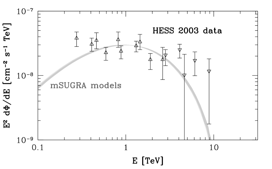
Figure 1: Minimal supergravity models of the annihilation flux fit to the 2004 HESS data. The grey band consists of several spectra generated with mSUGRA neutralinos of mass $\sim 11$ TeV.

We find that there is a family of mSUGRA models that produce a neutralino with a mass of 10 to 11 TeV consistent with current constraints and have a decent agreement with the HESS spectrum, with a $\chi^{2}$ of $\sim$ 1.2. These models require the $J$ parameter to be in the range [300,3000] BUBU to explain the flux observed by HESS.

Lower values of $J$ may be obtained once the parameter space is relaxed beyond mSUGRA. The difficulty in finding mSUGRA models that fit the HESS data lies in the excessive thermal relic densities predicted for neutralinos with the required mass, $\sim 10$ TeV or higher. Profumo Profumo (2005) has suggested that resonant annihilation of neutralinos through the A boson in the early Universe, which can occur for $m_{\rm A}\simeq 2m_{\chi}$, can lower the relic density for particles around 10 TeV. In this case the value of $J$ can be as low as $\sim 1600$ BUBU (see his Fig. (7b) obtained in an anomaly mediated supersymmetry breaking model) or even $\sim 3$ BUBU (see his Fig. 8b, for a generic MSSM model).

A third example of WIMPs that fit the HESS data are Kaluza-Klein particles. Ref. Bergström et al. (2005) finds that the spectrum for a model of KK DM requires a $J$ value of $\sim 130$ BUBU in order to be responsible for the flux recorded by HESS.

II.2 DM density profile

A dark matter density profile that would explain the TeV gamma-ray flux from the Galactic Center with the particles discussed in the last section will need to have a higher than expected density. The HESS GC source does not extend beyond $\sim 0.1^{\circ}$ or $\sim 10$ pc, covering a solid angle $\Omega\sim 10^{-5}$ sr. The required $J$ value from section II.1 ranges from $3-3000$ BUBU or a $dJ/d\Omega\sim 10^{5}-10^{8}$ BUBU sr^-1 for $0.1^{\circ}$ or $\Theta\sim 10^{-3}$ rad.

The contribution from the extended DM halo along the line of sight to the GC can be estimated from Eq. (5) as $dJ/d\Omega\sim\rho^{2}D$. For a canonical isothermal halo $\rho\sim 2~{}\rho_{local}\sim 0.6$ GeV cm^-3 and $dJ/d\Omega\sim 4$ BUBU sr^-1 from the DM column through the extended DM halo. This is $5$ to $8$ orders of magnitude smaller than required, so higher DM densities are needed to produce the gamma-ray flux by annihilation of our candidate DM particles.

A Navarro-Frenk-White profile (NFW) Navarro et al. (1997) is denser at the center. For an NFW profile, the average value of $dJ/d\Omega$ within $0.1^{\circ}$ is, from Eq. (16) below,

$$\frac{dJ}{d\Omega}\sim\frac{1}{\Omega}\int_{\Omega}\frac{dJ}{d\Omega}d\Omega=\frac{2\pi\rho_{s}^{2}r_{s}^{2}}{D\Theta}\sim 3\times 10^{3}~{}{\rm BUBU~{}sr^{-1}}.$$ (14)

This is still $2$ to $5$ orders of magnitude too small to explain the observed gamma ray flux for most of the dark matter particles we consider. We conclude that, if the HESS signal is due to DM annihilation, the extended halo contributes no more than a few percent of the gamma-ray flux and a strong enhancement in the density must exist within $10$ pc of the center of the galaxy.

The dark matter density profile within $10$ pc of the Galactic Center is not known in detail and mechanisms for such density enhancements have been proposed. For example, such enhancement could be explained by extreme clumping of the dark matter Silk and Stebbins (1993); Kolb and Tkachev (1994); Bergström, Edsjö, Gondolo, and Ullio (1999); Aloisio et al. (2004) which would have implications on models of structure formation, by steeper density profiles, $\rho\propto r^{-\alpha}$ with $\alpha\geq 3/2$, have been suggested Gurevich and Zybin (1995) but are disfavored, or by a strong dark matter concentration at the Galactic Center (a spike Gondolo and Silk (1999); Ullio, Zhao, and Kamionkovski (2001); Merritt et al. (2002); Gnedin and Primack (2004); Bertone and Merritt (2005, 2005)). To include the latter two possibilities, we split the dark matter profile into an inner and an outer part at a transition radius R_I.

As an example of the outer profile we use the NFW profile

$$\rho_{\rm NFW}=\frac{\rho_{s}}{\frac{r}{r_{s}}\left[1+\left(\frac{r}{r_{s}}\right)^{2}\right]}.$$ (15)

$r_{s}$ is a scale radius and $\rho_{s}$ is twice the density at $r_{s}$. We will take typical values Bergström, Ullio, and Buckley (1998) of $r_{s}=25$ kpc and $\rho_{s}=\rho_{0}(D/r_{s})[1+(D/r_{s})^{2}]$ with a local density $\rho_{0}=0.3$ GeV cm^-3. We take the distance to the Galactic Center to be $D=8$ kpc Reid (1993). For this profile we compute

$$\frac{dJ_{\rm NFW}}{d\Omega}=\rho_{s}^{2}r_{s}\left\{\frac{\pi-\theta}{y}-\frac{3+2y^{2}}{2(1+y^{2})}\left[\arctan\left(\frac{z}{\sqrt{1+y^{2}}}\right)+\frac{\pi}{2}\right]-\frac{z}{2(1+x^{2})(1+y^{2})}\right\}$$ (16)

where $\theta$ is the angle between the line of sight and the GC, $x=D/r_{s}$, $y=x\sin\theta$, and $z=x\cos\theta$.

Notice that Eq. (16) diverges in the direction of the GC ($\theta=0,y=0$) as $\pi\rho_{s}^{2}r_{s}^{2}/D\theta$. To remove the inner part of the NFW profile, we add an inner cutoff at $R_{\rm I}$ by replacing the term $(\pi-\theta)/y$ in Eq. (16) with

$${\cal F}(y,z_{c})+{\cal F}(y,b_{c})-\frac{z_{c}}{(1+y^{2})(1+x_{c}^{2})}-\frac{3+2y^{2}}{(1+y^{2})^{\frac{3}{2}}}\arctan\left(\frac{z_{c}}{\sqrt{1+y^{2}}}\right)$$ (17)

where $x_{c}=R_{\rm I}/r_{s}$, $z_{c}=\sqrt{x_{c}^{2}-y^{2}}$, $b_{c}=(zz_{c}+y^{2})/(z-z_{c})$, and

$${\cal F}(y,a)=\frac{1}{\sqrt{a^{2}+y^{2}}}\,{}_{2}F_{1}\!\left(\frac{1}{2},\frac{1}{2};\frac{3}{2};\frac{y^{2}}{y^{2}+a^{2}}\right)=\frac{1}{y}\arctan\!\left(\frac{y}{a}\right)$$ (18)

The form with the hypergeometric function is used to avoid division by zero at $y=0$ ($\theta=0$).

In the inner ($r\lesssim 10$ pc) part of the density profile we use a simple functional form to model a central density enhancement. We assume that a DM mass $M_{\rm I}$ is contained within a sphere of radius $R_{\rm I}$, and that its density profile is spherically symmetric and decreases with a power $\alpha$ of the radius. The inner profile we use is

$$\rho_{\rm I}(r)=\begin{cases}\displaystyle\frac{3-\alpha}{4\pi}\,\frac{M_{\rm I}}{R_{\rm I}^{3}}\left(\frac{r}{R_{\rm I}}\right)^{-\alpha},&R_{c}\leq r\leq R_{\rm I},\\ 0,&{\rm otherwise}.\end{cases}$$ (19)

This inner profile could be a steep profile, or a spike around the central black hole. For this inner profile, we find

$$J_{\rm I}=\frac{(3-\alpha)^{2}}{4\pi}\frac{M_{\rm I}^{2}}{R_{\rm I}^{3}D^{2}}\frac{1}{3-2\alpha}\left[1-\left(\frac{R_{c}}{R_{\rm I}}\right)^{3-2\alpha}\right].$$ (20)

Here R_c is an inner cutoff radius discussed in the next paragraph. For the angular profile we compute

$$j(\theta)\equiv\frac{1}{J}\frac{dJ(\theta)}{d^{2}\theta}=\begin{cases}\displaystyle\frac{1}{2\pi}\frac{3-2\alpha}{\theta_{\rm I}^{3-2\alpha}-\theta_{c}^{3-2\alpha}}\Bigg{[}\frac{\theta_{\rm I}^{1-2\alpha}}{1-2\alpha}\,F\!\left(\alpha,\frac{\theta}{\theta_{\rm I}}\right)-\frac{\theta_{c}^{1-2\alpha}}{1-2\alpha}\,F\!\left(\alpha,\frac{\theta}{\theta_{c}}\right)\Bigg{]},&\theta<\theta_{c},\\ \displaystyle\frac{1}{2\pi}\frac{3-2\alpha}{\theta_{\rm I}^{3-2\alpha}-\theta_{c}^{3-2\alpha}}\Bigg{[}\frac{\theta_{\rm I}^{1-2\alpha}}{1-2\alpha}\,F\!\left(\alpha,\frac{\theta}{\theta_{\rm I}}\right)-\frac{\theta^{1-2\alpha}}{1-2\alpha}\frac{\sqrt{\pi}\ \Gamma(\alpha+\frac{1}{2})}{\Gamma(\alpha)}\Bigg{]},&\theta_{c}<\theta<\theta_{\rm I},\end{cases}$$ (21)

and zero for $\theta>\theta_{\rm I}$. Here we defined $\theta_{\rm I}=R_{\rm I}/D$, $\theta_{c}=R_{c}/D$, and

$$F(\alpha,x)=\sqrt{1-x^{2}}\ _{2}F_{1}(\alpha,1;\alpha+\frac{1}{2};x^{2})$$ (22)

where ${}_{2}F_{1}$ is the hypergeometric function. Notice that for $\alpha=3/2$ the factor in front of the square bracket is $[2\pi\ln(\theta_{\rm I}/\theta_{c}]^{-1}$ and that for $\alpha=1/2$ the square bracket is $\ln(\theta_{\rm I}/\theta_{c})$.

An inner cutoff at $R_{c}$ is introduced to avoid the divergence that occurs in $dJ_{\rm I}/d\Omega$ when $\alpha\geq 3/2$. This inner cutoff is left as a free parameter, because this part of the halo is even more unknown than the rest. Physically an inner cutoff would naturally be present. Either the capture radius of the black hole, or some effective radius at which, e.g., the DM density is depleted by annihilation during the history of the Milky Way. In the latter case the maximum sustainable density is usually taken as

$$\rho~{}\leq~{}\rho_{max}~{}\simeq~{}\frac{m}{\langle\sigma v\rangle t}$$ (23)

with the time $t$ taken as the age of the Milky Way. In the case we are considering, we have a measurement of the flux and of the particle mass from the extent of the spectrum. For example, integrating Eq. (7) in energy above the threshold and inserting Eq. (19) with $\alpha=0$, Eq. (23) implies

$$M_{\rm I}~{}\geq~{}M_{c}~{}\equiv~{}\frac{8\pi D^{2}mt\Phi}{N_{\gamma}},$$ (24)

where $\Phi$ is the total photon flux above threshold and $N_{\gamma}$ is the number of photons produced above threshold in each annihilation. Thus the maximum density $\rho_{max}$ corresponds to a lower limit on the mass of an inner feature of the halo that could explain the gamma-ray observation. If the mass is too small, then the cross-section and density required to mantain the same flux are so large that the feature would have annihilated by now. This can be generalized to all $\alpha$ values by finding the $R_{c}$ for which $\rho(R_{c})\leq\rho_{max}$. They are any $R_{c}$ greater than the solution for $R_{q}$ in the equation

$$R=R_{q}\left(1+\frac{M_{c}^{2}}{D^{2}J}\frac{3-2\alpha}{4\pi R_{q}^{3}}\right)^{\frac{1}{3-2\alpha}}.$$ (25)

Another scale in this problem is the capture radius of a 3 million solar mass black hole, expected to be in the center of all of these profiles. We find that the capture radius, $\sim 10^{-7}$ pc, is greater than all $R_{q}$.

Thus, as a physically motivated number, we take the range of cutoff radii to be

$$10^{-7}~{}{\rm pc}\leq R_{c}\leq R_{\rm I}.$$ (26)

II.3 Limits from the HESS angular profile

The angular distribution of photons in the HESS detector carries information on the source profile. Here we investigate the constraint on the source profile due to these data.

The HESS analysis Aharonian et al. (2004) assumes a gaussian source profile, and gives a limit on the source angular size equal to $\leq 3^{\prime}$. To determine the limit on our power-law sphere in Eq. (19), we compare the emission profile, Eq. (21),with the angular distribution of detected photons. Fig. (2) in Aharonian et al. (2004) gives the photon counts $C_{i}$ and their errors $\delta_{i}$ in each $\theta_{i}^{2}$ bin. Here $\theta_{i}$ is the angle between the photon direction and the center of the excess. The center of the excess agrees to the position of the GC to well within the systematic errors in the pointing of the HESS array. The intrinsic angular profile

$$j(\theta)=\frac{1}{J}\left[\frac{dJ_{\rm I}}{d\Omega}+\frac{dJ_{\rm o}}{d\Omega}\right]$$ (27)

is convolved with the point spread function (psf) of HESS as given in Horns (2005):

$$f_{psf}(\theta)=f_{0}\left[e^{-\frac{\theta^{2}}{2\sigma_{1}^{2}}}+\frac{1}{8.7}e^{-\frac{\theta^{2}}{2\sigma_{2}^{2}}}\right].$$ (28)

Here $f_{0}$ was chosen so the psf has unit area and the widths of the gaussians are $\sigma_{1}$ = 0.052^∘ and $\sigma_{2}$ = 0.136^∘. We rewrite this as a linear combination of two normalized gaussians,

$$f_{psf}(\theta)=\frac{c_{1}}{2\pi\sigma_{1}^{2}}e^{-\frac{\theta^{2}}{2\sigma_{1}^{2}}}+\frac{c_{2}}{2\pi\sigma_{2}^{2}}e^{-\frac{\theta^{2}}{2\sigma_{2}^{2}}}$$ (29)

with $c_{1}=8.7\sigma_{1}^{2}/(8.7\sigma_{1}^{2}+\sigma_{2}^{2})$ and $c_{2}=\sigma_{2}^{2}/(8.7\sigma_{1}^{2}+\sigma_{2}^{2})$. The source profile convolved with a normalized gaussian is

$$\overline{j}(\theta,\sigma)=\sigma^{-2}e^{-\frac{1}{2}(\frac{\theta}{\sigma})^{2}}\int_{0}^{\theta_{DM}}\theta^{\prime}e^{-\frac{1}{2}(\frac{\theta^{\prime}}{\sigma})^{2}}I_{0}\Big{(}\frac{\theta\theta^{\prime}}{\sigma^{2}}\Big{)}j(\theta^{\prime})d\theta^{\prime}$$ (30)

and $j$ convolved with the entire psf is

$$j_{psf}(\theta)=c_{1}\overline{j}(\theta,\sigma_{1})+c_{2}\overline{j}(\theta,\sigma_{2}).$$ (31)

The photon counts $C(\theta)$ as a function of angle $\theta$ from the GC are proportional to the convolution of $dJ/d\Omega$ with the psf

$$C(\theta)=A\left(\frac{dJ}{d\Omega}\right)_{\rm psf}.$$ (32)

The proportionality constant is given by

$$A={\cal E}\frac{\langle\sigma v\rangle}{m_{\chi}^{2}}\frac{N_{\gamma}}{8\pi}\pi\Delta\theta^{2},$$ (33)

where ${\cal E}$ is the exposure, $N_{\gamma}$ is the total number of photons

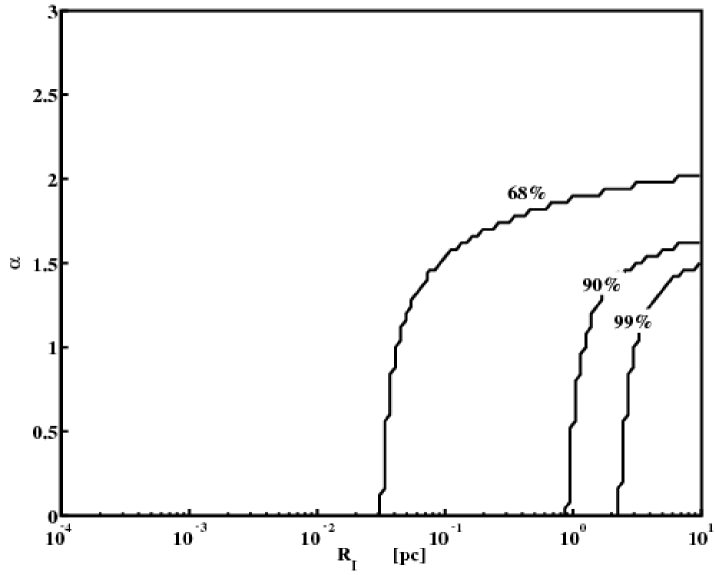
Figure 2: The constraint from the HESS angular size. The profiles are generally required to be steep, $\alpha>1.5$, or small, $R_{\rm I}<1$ pc.

above the experimental threshold emitted per annihilation, and $\Delta\theta^{2}$ is the aperture of the observation. We have estimated the HESS exposure as the ratio of the total counts assuming a point source and the integral flux of $1.82\times 10^{-6}$m^-2s^-1 above threshold, both as reported by HESS in Aharonian et al. (2004). We estimate an exposure ${\cal E}\sim 3\times 10^{13}$ cm² s. Furthermore,

$$\left(\frac{dJ}{d\Omega}\right)_{\rm psf}=J\,j_{\rm psf}(\theta).$$ (34)

The best fit for the normalization factor $A$ is

$$A=\sum_{i}\frac{C_{i}\,J\,j_{psf}(\sqrt{\theta^{2}_{i}})}{\delta_{i}},$$ (35)

with the $\chi^{2}$ given by

$$\chi^{2}=\sum_{i}\Bigg{(}\frac{C_{i}-AJj_{psf}(\sqrt{\theta^{2}_{i}})}{\delta_{i}}\Bigg{)}^{2}.$$ (36)

Here to find our intervals we perform a bayesian analysis. We take the likelihood as proportional to $e^{-\chi^{2}/2}$ and define our confidence intervals in $(\alpha,R_{\rm I})$ as the corresponding quantiles of the posterior distribution. We take the prior distribution as flat in $\log R_{\rm I}$ and $\alpha$, and zero outside the range shown in Fig. (2).

The intermediate results of this piece of the analysis are shown in Fig. (2). The $68\%$, $90\%$, and $99\%$ regions in the ${R_{\rm I},\alpha}$ are shown. At the $90\%$ confidence level the HESS data confines the source diameter to $\lesssim 1$ pc for a uniform sphere. For power law density profiles with index $\alpha\gtrsim 1.5$ the constraint on the source size starts to weaken considerably; these profiles could be modeled as a smaller source with a harder power law index.

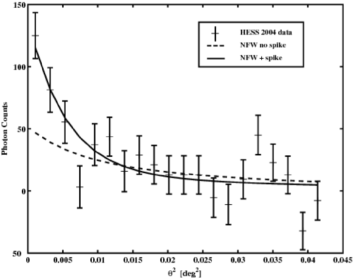
Figure 3: An NFW+spike fit to the 2004 HESS gamma-ray data on the Galactic Center. For this fit we used a NFW profile outside $1$ pc and a $\rho\sim r^{-1.9}$ profile for $r<1$ pc. An inner cutoff of $10^{-5}$ pc was used to approximate the inner core. This is a typical profile of a spike after dynamical heating and annihilation effects are included.

Finally, we include a fit of two profiles in Fig. (3). The first, more shallow profile is an NFW profile alone. Evidently the flux rules out an NFW only DM profile, and so does the angular profile of the gamma-ray source. The steeper profile is a fit of an NFW profile with a spike. A spike can simulate a point source effectively, and the extended NFW piece makes the profile fit slightly better than a point source.

As an illustration of the kind of angular gamma-ray profiles compatible with the HESS data in models with a DM spike we show such a profile for an NFW model. We fix the halo NFW model with the parameters give in section II.2. A pure NFW model does not fit the data well at small angles from the GC. However, motivated by Gondolo and Silk (1999), we add a spike with a radius of $1$ pc and a slope of $\alpha=1.9$, which are typical values after inclusion of the effects of stars and annihilation Bertone and Merritt (2005). The $\chi^{2}$ per degree of freedom for the fit is $1.3$ which is the same ($\Delta\chi^{2}\sim 10^{-4}$) as in the fit of a point-like source. Since the density of the dark matter is fixed for this profile is fixed to the local density and the particle mass is bounded by the spectrum, the normalization of the fit to the flux gives the value of the cross-section, $N_{\gamma}\langle\sigma v\rangle=3.3\times 10^{-28}$ cm³ s^-1. This is a reasonable value for the WIMP annihilation cross section in particle physics models.

II.4 Limits from stellar dynamics mass measurements

Measurements of the amount of mass $M(<r)$ contained within a distance $r$ from the GC are continuously improved as more precise data are collected. Here we use the compilation of enclosed mass measurements in Ghez et al. (2003). From their paper, we extract a table of the mass $M_{i}$ contained within radius $r_{i}$, together with its quoted error $\sigma_{i}$.

To these data we fit a mass profile with three components: the central black hole, the central stellar cluster, and the dark matter sphere described above.

$$M(<r)=M_{\rm BH}+M_{*}(<r)+M_{\rm I}(<r).$$ (37)

$M_{\rm BH}$ is the mass of the central black hole Sagittarius A^∗. For the central stellar cluster we use the empirical mass profile $M_{*}(<r)$ obtained from data in Genzel et al. (2003),

$$M_{*}(<r)=\begin{cases}\displaystyle M_{*}\left(\frac{r}{R_{*}}\right)^{1.6},&r\leq R_{*},\\ \displaystyle M_{*}\left(\frac{r}{R_{*}}\right)^{1.0},&r>R_{*},\end{cases}$$ (38)

with $M_{*}=0.88\times 10^{6}M_{\odot}$ and $R_{*}$ = 0.3878 pc. We model the dark matter with the density profile described in Eq (19), which corresponds to a DM mass profile

$$M_{\rm I}(<r)=\begin{cases}\displaystyle M_{\rm I}\left(\frac{r}{R_{\rm I}}\right)^{3-\alpha},&r\leq R_{\rm I},\\ \displaystyle M_{\rm I},&r>R_{\rm I}.\end{cases}$$ (39)

We use the likelihood function to find constraints on the DM density profile, using a bayesian analysis similar to section II.3. Assuming the errors quoted in Ghez et al. (2003) are gaussian, the likelihood ${\cal L}$ is given by

$$2\ln{\cal L}=\sum_{i}\frac{(M_{i}-M(<r_{i}))^{2}}{\sigma_{i}^{2}}=\sum_{i}\frac{(M_{i}-M_{\rm BH}-M_{*}(<r_{i})-M_{\rm I}f_{i})^{2}}{\sigma_{i}^{2}}$$ (40)

with

$$f_{i}=\begin{cases}\displaystyle\left(\frac{r_{i}}{R_{\rm I}}\right)^{3-\alpha},&r_{i}\leq R_{\rm I},\\ \displaystyle 1,&r_{i}>R_{\rm I}.\end{cases}$$ (41)

In order to obtain a constraint on the parameters $M_{\rm I}$ and $R_{\rm I}$ at a fixed value of $\alpha$, we first marginalize over $M_{BH}$. Since $\ln{\cal L}$ is quadratic in $M_{BH}$, we need only replace $M_{BH}$ in Eq. (40) with the value $M_{BH}^{0}$ obtained by maximizing the likelihood. This is given by

$$M_{BH}^{0}=\frac{x_{3}x_{4}-x_{2}x_{5}}{x_{3}^{2}-x_{1}x_{5}},$$ (42)

with

$$x_{1}=\sum\frac{1}{\sigma_{i}^{2}},\quad x_{2}=\sum\frac{M_{i}-M_{*}(<r_{i})}{\sigma_{i}^{2}},\quad x_{3}=\sum\frac{f_{i}}{\sigma_{i}^{2}},\quad x_{4}=\sum\frac{f_{i}[M_{i}-M_{*}(<r_{i})]}{\sigma_{i}^{2}},\quad x_{5}=\sum\frac{f_{i}^{2}}{\sigma_{i}^{2}}.$$ (43)

As our prior, $R_{\rm I}$ is restricted to the range [0.0004,10] pc and distributed logarithmically, and $\alpha$ is kept at a few fixed values (0,1,2). By integrating our posterior probability distribution we derive a 1 sigma upper limit and a 90$\%$ bayesian interval in the $M_{\rm I}$, $R_{\rm I}$ parameter space. For $R_{\rm I}$ smaller than the innermost data point (0.0004 pc), there is a degeneracy between $M_{BH}$ and $M_{\rm I}$. We break this degeneracy by imposing $M_{\rm I}$ less than the upper bound on the black hole mass reported in Ghez et al. (2003) ($3.6\pm 0.4\times 10^{6}M_{\odot}$). This is equivalent to assuming all the mass within the innermost orbit could be DM.

III Results

From the particle examples in Section II.1 we find that a range of $J=[300,3000]$ is needed to explain the flux of gamma-rays from the GC as DM annihilation products. With resonant annihilations, $J$ can be as low as $\sim 1$. Furthermore we conclude that the DM annihilation line will be unobservable with an energy resolution of $10\%$. We find that the spectrum of gamma rays from the GC is compatible with the decay of pions produced in the annhilation. More complex models of the radiation, such as Bergström et al. (2005) where bremsstrahlung of $W$ products has an appreciable effect, the spectrum may be similar to a power law and other spectral features, such as a hardening of the spectrum near the WIMP mass, may be observable.

The requirement that the central feature of dark matter not annihilate in the lifetime of the Universe gives a lower limit on the mass. For example, a central feature with $\alpha=0$ and an upper limit on the density of $\rho=10^{15}$ M_⊙ pc^-3 and the requirement that $J=1000$ BUBU gives a lower limit of $\sim 3\times 10^{-4}$ M_⊙. For a limit density of $\rho=10^{12}$ M_⊙ pc^-3 the mass of annihilating dark matter must be greater than $\sim 1$ M_⊙ to be stable for $10^{10}$ years. These limits are below the lower edge of our results plots.

The stellar dynamics limit extended mass distributions to $\sim 10\%$ of the black hole mass for $R_{\rm I}=(10^{-3},1)$. The angular size bounds are complementary excluding regions above a radius that depends on the assumed $\alpha$ for the distribution, as seen in Fig. (2).

The results of the analysis are compiled in Figs. (4, 5, 6, and 7). In Figs. (4, 5, 6) we plot both the stellar dynamics bound and the angular size bound in the $M_{\rm I}-R_{\rm I}$ plane for three values of $\alpha$. The expected range from the particle physics are shown as shaded regions. These regions correspond to either a value of $J$ that could produce the observed flux, or equivalently to a value for $N\langle\sigma v\rangle$.

Comparing these models to our stellar dynamics bounds, we see that for $\alpha=0$ (Fig. 4) the source size is restricted to $\lesssim 20$ pc in mSUGRA and KK models. For larger cross-sections with resonant annihilation, the source size is unbounded by the stellar dynamics. The constraint from the HESS source profile limits the source size to $\lesssim 1$ pc (vertical line), so it is similar to the stellar dynamics constraint in mSUGRA and KK models, but is stronger for resonant-annihilation models. However, for some of the mSUGRA models we considered the stellar dynamics constrains were stronger restricting the source size to $\lesssim 0.3$ pc.

For profiles with shallow cusps ($\alpha=1$; Fig. 5), the source size constraint on WIMP models from stellar dynamics is similar to the $\alpha=0$ case. No bounds for resonant-annihilation models, but still $\lesssim 20$ pc for mSUGRA and KK models. The HESS constraint from the angular size of the gamma-ray excess is still $\sim 1$ pc and so conclusions similar to those with $\alpha=0$ apply in this case.

For profiles with steep cusps ($\alpha=2$; Fig. 6) stellar dynamics bounds out to $10$ pc do not provide a constraint on the WIMP models we examined. The constraint from the HESS angular profile is also much weaker here. We show two plots here to illustrate the effect of the cutoff radius which only comes into play for these steep profiles. We show two cutoff radii of $10^{-4}$ and $10^{-6}$ pc.

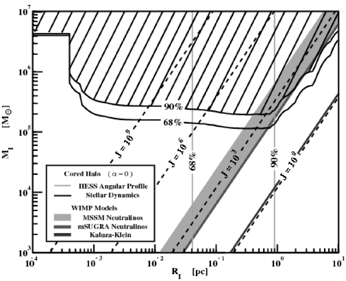
Figure 4: Stellar orbit constraints on the mass and size of a dark matter concentration at the Galactic center. The black lines are the $1$ sigma upper limit and $90\%$ confidence interval for the mass of dark matter spheres with power law density profile index $\alpha=0$. The dashed lines show the mass corresponding to the $J$ values indicated (in BUBU). The $1$ sigma and $90\%$ bounds from the angular profile are shown as the vertical gray lines. The grey bands show the typical values of $J$ required to produce the HESS flux in WIMP models: KK (dark grey), mSUGRA (medium grey), and MSSM (light grey)

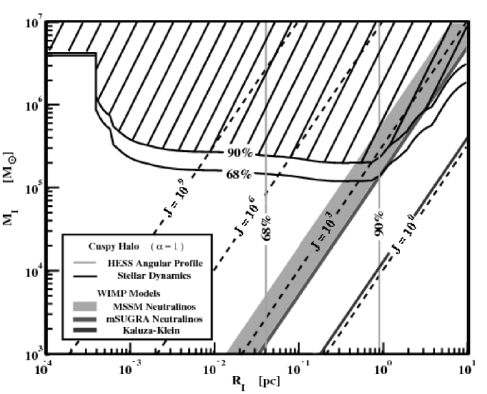
Figure 5: Same as Fig. (4) but for dark matter spheres with power law density profiles with $\alpha=1$.

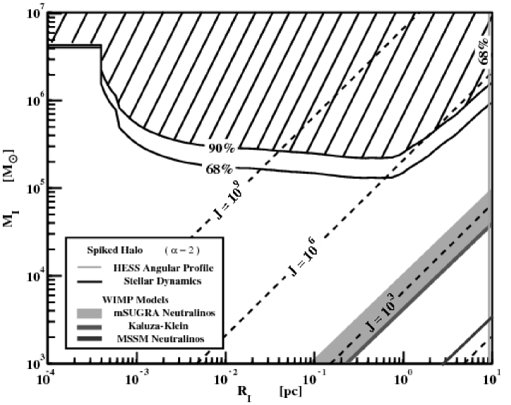
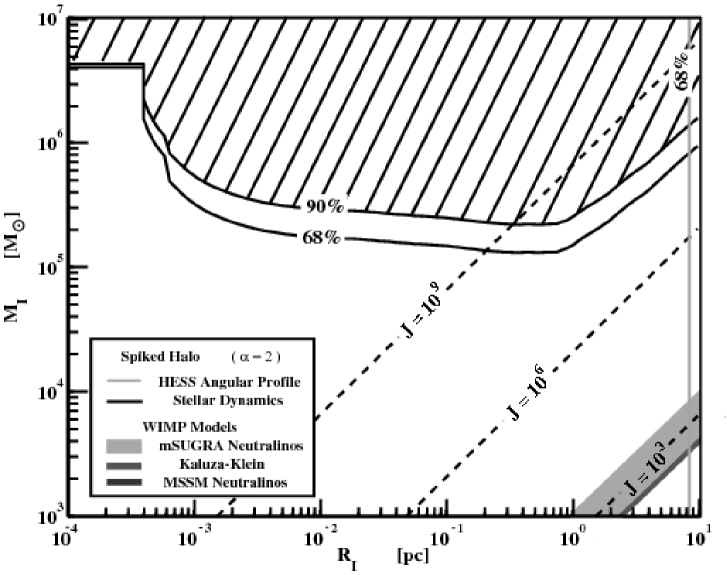
Figure 6: Same as Fig. (4) but for inner DM profiles with $\alpha=2$. For this steep density profile, which “looks” like a smaller sphere, the size constraint on the DM feature is not as strong, constraining values of $J\sim 10^{6}$ BUBU or higher. To avoid a divergence in $J$ and because these profiles are expected to flatten at some inner radius, these profiles were computed with a minimum cutoff radius $R_{c}=10^{-4}$ pc (top) and $R_{c}=10^{-6}$ pc (bottom).

The constraints from stellar orbits and the HESS angular distribution are summarized for comparison in figure 7. The solid line represents the $90\%$ confidence region based on the HESS data alone. The dotted lines show the constraint coming from stellar dynamics. Various values of $J$ are plotted so that these constraints can be compared to particle physics models. The values of $J$ required by the mSUGRA neutralinos, MSSM neutralinos, and Kaluza-Klein particles we examined are plotted as the medium grey band. Both the stellar dynamics and the gamma-ray angular profile point to a DM source that is either small or steep.

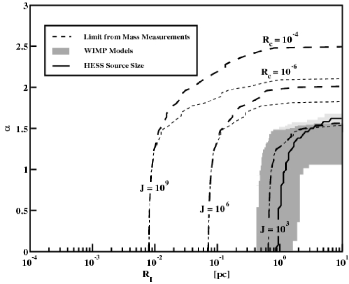
Figure 7: Constraints on the $J$ parameter due to stellar orbit data Ghez et al. (2003); Genzel et al. (2003) and the HESS source profile. The dashed lines show the crossing of specific $J$ values with the $90\%$ confidence level from stellar orbit measurements as shown in Figs. (4,5, and 6) for specific values of $\alpha$. The $90\%$ constraint on the source profile from the HESS data alone is shown as the solid line. The grey band is the expected range of $J$ for mSUGRA neutralinos that produce the GC TeV flux.

IV Conclusions

To summarize, a very high energy gamma-ray flux from the center of the Milky Way was significantly detected by the HESS collaboration during 2003-2004. A possible explanation of the very high energy radiation from the Galactic Center is WIMP annihilation. The intensity of the annihilation flux is a function of the density profile of dark matter in the galactic center. The angular distribution of detected gamma rays limits the size of the emission region. Data on on the proper motions of stars and star counts around the galactic center constrain the size and the mass of the dark matter at the GC. We have shown that the density needed to produce the observed flux from WIMP annihilation is consistent with observational constraints on the mass profile of the GC. For the stellar orbit data and the star counts, we used the infrared data in Ghez et al. (2003) and Genzel et al. (2003). We found that these astronomical constraints on the source profile are comparable to and slightly stronger than the constraint from the angular distribution of photons measured by HESS.

There are several ways in which WIMP annihilation as the origin of the HESS flux could be confirmed or made implausible. As is clear from fig. 7, a slight improvement in either the gamma-ray angular resolution or the constraints from stellar orbits may reveal the presence of an extended dark matter annihilation region at the Galactic Center. An extended emission out to large angles would be a possible indication of WIMP annihilation. An extended gamma-ray excess with the same spectrum and position of the GC flux has recently been reported by HESS Aharonian et al. (2006). A spectral cutoff at energies higher than the particle mass is another requirement of the DM hypothesis. The cutoff may be preceded by a gamma-ray line at the particle mass, but this spectral line does not appear to be observable with atmospheric Cherenkov telescopes in the particle models we examined due to the insufficient energy resolution. Absence of variability is another feature of WIMP annihilation, thus variability of the source would be difficult to reconcile with the DM interpretation of the GC TeV flux. Finally, since the dark matter permeates our Universe, if the same radiation was found in the centers of other mass concentrations, population studies may be possible that could help confirm or deny the annihilation nature of this radiation Vassiliev et al. (2003).

A small spike on an NFW profile could explain the large gamma-ray flux which is not expected from cored or cusped halos. Astrophysically small spikes in the DM halos are not favored, but not ruled out either. The infrared data of proper motions in the GC show about three million solar masses confined to a space of 90 AU. The compression of this baryonic matter may adiabatically compress the dark matter and lead to such a spike in the profile Gondolo and Silk (1999). Any merger events with larger stellar sized objects should dynamically heat the DM spike reducing its density.

Further observations of the Galactic Center in gamma rays are ongoing. There are hints that the TeV radiation from the Galactic Ridge is connected to the Galactic Center point source. The TeV flux from the GC seems to be constant in time and a cutoff in the spectrum (now reported to have a spectrum with $\alpha=2.4$) has not been found up to energies of $\sim 6$ TeV Rolland et al. (2005), so the models considered here are still viable. The nature of this non-thermal radiation source in the center of the Milky Way is still unknown and undergoing active study and observations.

Acknowledgements. This work was supported in part by NSF grant PHY-0456825 and NSF grant #0079704. We thank Mark Morris for useful discussions and Ted Baltz for providing us with a collection of minimal supergravity models with heavy neutralinos.

References

- Zwicky (1933) F. Zwicky, Helv.Phys.Acta., 6, 110 (1993).
- Babcock (1939) H.W. Babcock, 1939LicOB, 19, 41B (1939).
- Bennett et al. (2003) C.L. Bennett et al., ApJS, 148, 1 (2003).
- Cyburt et al. (2003) R.H. Cyburt, B.D. Fields, K.A. Olive, Phys.Lett., B567, 227-234 (2003).
- Tonry et al. (2003) J.L. Tonry et al., Astrophys.J., 594, 1-24 (2003).
- Spergel et al. (2006) D.N. Spergel et al., astro-ph/0603449(2006)
- Benbow et al. (2004) W. Benbow for the H.E.S.S. Collaboration, 2nd Int. Symp. on High Energy Gamma Ray Astronomy, Heidelberg, APS Conf. Proc. 745, p. 468 (2004).
- Silk and Bloeman (1987) J. Silk and H. Bloemen, ApJ, 313L, 47S (1987).
- Stecker and Tylka (1989) F.W. Stecker and A.J. Tylka, ApJ, 343, 169S (1989).
- Flores and Primack (1994) R.A. Flores and J.R. Primack, ApJ, 427L, 1F (1994).
- Mayer-Hasselwander et al. (1998) H.A. Mayer-Hasselwander et al. A&A, 335, 161M (1998).
- Bergström, Ullio, and Buckley (1998) L. Bergström, P. Ullio, and J. Buckley, Astropart.Phys. 9 (1998) 137-162.
- Gondolo and Silk (1999) P. Gondolo and J. Silk, Phys.Rev.Lett. 83 (1999) 1719-1722.
- Cesarini et al. (2004) A. Cesarini et al., APh, 21, 267C (2004).
- Evans et al. (2004) N.W. Evans, F. Ferrer, and S. Sarkar, Phys.Rev. D69 (2004) 123501.
- Kosack et al. (2004) K. Kosack et al., ApJ, 608, (2004) L97.
- Tsuchiya et al. (2004) K. Tsuchiya et al., ApJ, 606, (2004) L115.
- Hofmann et al. (2003) W. Hofmann, Proc. 28th ICRC, Tsukuba, Univ. Academy Press, Tokyo, (2003) p.2811.
- Ghez et al. (2005) A.M. Ghez et al., ApJ, 620, (2005) 744.
- Aharonian et al. (2004) F.A. Aharonian et al., A&A 425 (2004) L13-L17.
- Aharonian et al. (2004) F.A. Aharonian et al., Nature 432 (2004) 75.
- Aharonian et al. (2005) F.A. Aharonian et al., A&A 432 (2005) L25-L29.
- Atoyan and Dermer (2004) A. Atoyan, C. Dermer, ApJ, 617 (2004) L123-L126.
- Aharonian et al. (2004) F.A. Aharonian et al., Astrophys.J. 619 (2005) 306-313.
- Horns (2005) D. Horns, Phys.Lett. B607 (2005) 225-232; Erratum-ibid. B611 (2005) 297.
- Bergström et al. (2005) L. Bergström, T. Bringmann, M. Eriksson, M. Gustafsson Phys.Rev.Lett. 94 (2005) 131301.
- Ullio, Zhao, and Kamionkovski (2001) P. Ullio, H.S. Zhao, M. Kamionkowski, Phys. Rev. D, 64, (2001) 043504.
- Merritt et al. (2002) D. Merritt, M. Milosavljevic, L. Verde, and R. Jimenez. Phys. Rev. Lett., 88, (2002) 191301.
- Gnedin and Primack (2004) O.Y. Gnedin, J.R. Primack, Phys.Rev.Lett. 93 (2004) 061302.
- Bertone and Merritt (2005) G. Bertone, D. Merritt, Phys.Rev.D 72, (2005) 103502.
- Ghez et al. (1998) A.M. Ghez, B.L. Klein, M. Morris, and E.E. Becklin, ApJ, 509, (1998) 678G.
- Ghez et al. (2000) A.M. Ghez, M. Morris, E.E. Becklin, A. Tanner, and T. Kremenek, Nature, 407, 6802 (2000) 349-351.
- Morris (2004) M. Morris, Private communication.
- Ghez et al. (2003) A.M. Ghez et al., Astron.Nachr. 324 S1 (2003) 527G.
- Gondolo et al. (2004) P. Gondolo, J. Edsjö, P. Ullio, L. Bergström, M. Schelke and E.A. Baltz, JCAP 0407 (2004) 008.
- Gelmini et al. (2006) G. Gelmini, P. Gondolo, A. Soldatenko C. Yaguna, hep-ph/0605016 (2006)
- Gelmini and Gondolo (2006) G. Gelmini, P. Gondolo hep-ph/0602230 (2006)
- Bergström et al. (2005) L. Bergström, T. Bringmann, M. Eriksson, M. Gustafsson, Phys.Rev.Lett. 95, (2005) 241301.
- Profumo (2005) S. Profumo, Phys.Rev.D 72, (2005) 103521.
- Navarro et al. (1997) J. F. Navarro, C. S. Frenk, S. D. M. White, ApJ 490 (1997) 493.
- Silk and Stebbins (1993) J. Silk, A. Stebbins, Astrophys.J. 411, (1993) 439.
- Kolb and Tkachev (1994) E.W. Kolb, I. I. Tkachev, Phys.Rev.D 50, (1994) 769.
- Bergström, Edsjö, Gondolo, and Ullio (1999) L. Bergström, J. Edsjö, P. Gondolo, and P. Ullio, Phys.Rev.D 59 (1999) 043506.
- Aloisio et al. (2004) R. Aloisio, P. Blasi, A.V. Olinto, Astrophys.J. 601, (2004) 47.
- Gurevich and Zybin (1995) A.V. Gurevich, K.P. Zybin, Sov.Phys.Usp. 165, (1995) 723.
- Bertone and Merritt (2005) G. Bertone, D. Merritt, Mod.Phys.Lett.A 20, (2005) 1021.
- Reid (1993) M. Reid, ARA&A, 31, 345R (1993).
- Genzel et al. (2003) R. Genzel et al., ApJ 594, 812 (2003).
- Aharonian et al. (2006) F. Aharonian et al., Nature 439 (2006) 695-698.
- Vassiliev et al. (2003) V.V. Vassiliev for the VERITAS Collaboration, Proc. 28th ICRC, Tskuba, Japan (2003).
- Rolland et al. (2005) L. Rolland and J. Hinton for the HESS Collaboration, Proc. 29th ICRC, Pune, India (2005).