Detection of the ISW effect and corresponding dark energy constraints made with directional spherical wavelets

Abstract

Using a directional spherical wavelet analysis we detect the integrated Sachs-Wolfe (ISW) effect, indicated by a positive correlation between the first-year Wilkinson Microwave Anisotropy Probe (WMAP) and NRAO VLA Sky Survey (NVSS) data. Detections are made using both a directional extension of the spherical Mexican hat wavelet and the spherical butterfly wavelet. We examine the possibility of foreground contamination and systematics in the WMAP data and conclude that these factors are not responsible for the signal that we detect. The wavelet analysis inherently enables us to localise on the sky those regions that contribute most strongly to the correlation. On removing these localised regions the correlation that we detect is reduced in significance, as expected, but it is not eliminated, suggesting that these regions are not the sole source of correlation between the data. This finding is consistent with predictions made using the ISW effect, where one would expect weak correlations over the entire sky. In a flat universe the detection of the ISW effect provides direct and independent evidence for dark energy. We use our detection to constrain dark energy parameters by deriving a theoretical prediction for the directional wavelet covariance statistic for a given cosmological model. Comparing these predictions with the data we place constraints on the equation-of-state parameter $w$ and the vacuum energy density $\Omega_{\Lambda}$. We also consider the case of a pure cosmological constant, i.e. $w=-1$. For this case we rule out a zero cosmological constant at greater than the 99.9% significance level. All parameter estimates that we obtain are consistent with the standand cosmological concordance model values. Although wavelets perform very well when attempting to detect the ISW effect since one may probe only the regions where the signal is present, once all information is incorporated when computing parameter estimates, the performance of the wavelet analysis is comparable to other methods, as expected for a linear approach.

1 Introduction

Strong observational evidence now exists in support of the $\Lambda$ cold dark matter ($\Lambda$CDM) fiducial model of the universe; specifically, a universe that is (nearly) flat and dominated by an exotic dark energy component. We know very little about the origin and nature of this dark energy, but we now have strong evidence in support of its existence and relative abundance. Much of this evidence comes from recent measurements of the cosmic microwave background (CMB) anisotropies of high resolution and precision, in particular the recent Wilkinson Microwave Anisotropy Probe (WMAP) data (Bennett et al., 2003a). The existence of dark energy has also been independently found by measurements of the luminosity distance to Supernova Type Ia (Riess et al., 1998; Perlmutter et al., 1999).

At this point, the confirmation of the fiducial $\Lambda$CDM model and the existence of dark energy by independent physical methods is of particular interest. One such approach is through the detection of the integrated Sachs-Wolfe (ISW) effect (Sachs & Wolfe, 1967). CMB photons are blue and red shifted as they fall into and out of gravitational potential wells, respectively, as they travel towards us from the surface of last scattering. If the gravitational potential evolves during the photon propagation, then the blue and red shifts do not cancel exactly and a net change in the photon energy occurs. This secondary induced CMB anisotropy (the ISW effect) exists only in the presence of spatial curvature or, in a flat universe, in the presence of dark energy (Peebles & Ratra, 2003). The recent WMAP 1-year data has imposed strong constraints on the flatness of the universe (Bennett et al., 2003a; Spergel et al., 2003), hence any ISW signal may be interpreted directly as a signature of dark energy.

It is difficult to separate directly the contribution of the ISW effect from the CMB anisotropies, hence it is not feasible to detect the ISW effect solely from the CMB. Instead, as first proposed by Crittenden & Turok (1996), the ISW effect may be detected by cross-correlating the CMB anisotropies with tracers of the local matter distribution, such as the nearby galaxy density distribution. A detection of large-scale positive correlations is a direct indication of the ISW effect, and correspondingly, evidence for dark energy.

The first attempt to detect the cross-correlation between the CMB and the nearby galaxy distribution was performed by Boughn & Crittenden (2002) using the Cosmic Background Explorer-Differential Microwave Radiometer (COBE-DMR; Bennett et al. 1996) and NRAO VLA Sky Survey (NVSS; Condon et al. 1998) data. No cross-correlation was found; Boughn & Crittenden (2002) conclude that a future experiment with better sensitivity and resolution was required to make any detection. The WMAP mission has now provided a suitable experiment, and several groups have since reported detections of the ISW effect at a range of significance levels using various tracers of the local universe. Boughn & Crittenden (2004, 2005) cross-correlate the WMAP data with two different tracers of the nearby universe: the hard X-ray data provided by the High Energy Astronomy Observatory-1 satellite (HEAO-1; Boldt 1987) and the NVSS data. They make a statistically significant detection of the cross-correlation at the $1.8$–$2.8\sigma$ level at scales below $3^{\circ}$. Nolta et al. (2004) perform an independent analysis of the WMAP and NVSS data and confirm the existence of dark energy at the $95$% significance level. Fosalba & Gazta$\tilde{\rm n}$aga (2004) cross-correlate the WMAP data with the APM galaxy survey (Maddox et al., 1990) and report a cross-correlation detection at the $2.5\sigma$ level on scales of $4^{\circ}$–$10^{\circ}$. Fosalba et al. (2003) cross-correlate the WMAP data with the Sloan Digital Sky Survey (SDSS; York et al. 2000) and detect an ISW signal at the $3\sigma$ level. These same two data sets are also analysed by Scranton et al. (2003). Afshordi et al. (2004) cross-correlate the WMAP data with the near infrared Two Micron All Sky Survey Extended Source Catalogue (2MASS XSC; Jarrett et al. 2000) and detect an ISW signal at the $2.5\sigma$ level. Padmanabhan et al. (2004) make a $2.5\sigma$ detection of the ISW effect by cross-correlating the WMAP and SDSS data, and subsequently use the detection to constrain cosmological parameters. Other works have focused on the theoretical detectability of the ISW effect for various experiments and, in some cases, the use of such detections to constrain cosmological parameters (Afshordi, 2004; Hu & Scranton, 2004; Pogosian, 2004; Pogosian et al., 2005; Corasaniti et al., 2005).

The previous works discussed all perform the cross-correlation of the CMB with various tracers of the near universe large scale structure (LSS) in either real or harmonic space, using the real space angular correlation function or the cross-angular power spectrum respectively. Recently, Vielva et al. (2006) adopt a different measure by performing the cross-correlation in spherical wavelet space using the azimuthally symmetric spherical Mexican hat wavelet (SMHW). Spherical wavelets have already been used in many astrophysical and cosmological applications. For example, spherical wavelets have been used extensively to test the CMB for non-Gaussianity and isotropy (Barreiro et al., 2000; Cayón et al., 2001, 2003, 2005; Martínez-González et al., 2002; Vielva et al., 2004; Mukherjee & Wang, 2004; , Cruz et al.2005, Cruz et al.2006; McEwen et al., 2005b; Liu & Zhang, 2005; Wiaux et al., 2006). However, Vielva et al. (2006) present the first use of spherical wavelets for cross-correlating the CMB with tracers of LSS in an attempt to detect the ISW effect. Since the ISW effect is localised to certain (large) scales on the sky, wavelets are an ideal tool for searching for cross-correlations due to the inherent scale and spatial localisation afforded by a wavelet analysis. Vielva et al. (2006) examine the covariance of the SMHW coefficients of the WMAP and NVSS data for a range of scales, making a detection of the ISW effect at the $3.3\sigma$ level at scales on the sky of $6^{\circ}$–$8^{\circ}$. Moreover, the detection is used to constrain cosmological parameters that describe the dark energy.

There is no physical reason to assume that the local correlated structures induced in the CMB anisotropies by the near LSS are rotationally invariant; indeed, it is known that Gaussian random fields are characterised by features that are not necessarily rotationally invariant Barreiro et al. (1997, 2001). Thus, other spherical wavelets that are not azimuthally symmetric, i.e. directional wavelets, may be equally (or more) suitable for probing the data for cross-correlations. Herein we extend the analysis performed by Vielva et al. (2006), using directional wavelets to examine the cross-correlation of the WMAP and NVSS data. We use any detections of the ISW made to constrain cosmological parameters that describe the dark energy.

The remainder of this paper is structured as follows. The directional continuous spherical wavelet transform and the wavelets that we consider are described in section 2. In section 3 we define the wavelet covariance estimator used to test for correlations and also define the theoretical covariance predicted for a given cosmological model (the derivation for which is presented in Appendix A). We then compare the expected performance of various wavelets for detecting the ISW effect. In section 4 we give a brief overview of the data considered and the analysis procedure. Results are presented and discussed in section 5. We describe the detections made and then use the detections to place constraints on dark energy parameters. Concluding remarks are made in section 6

2 Continuous spherical wavelet transform

To perform a wavelet analysis of full-sky maps defined on the celestial sphere, Euclidean wavelet analysis must be extended to spherical geometry. A wavelet transform on the sphere has already been constructed and developed (Antoine & Vandergheynst, 1998, 1999; Antoine et al., 2002, 2004). The spherical wavelet construction is derived entirely from group theoretic principles, however recently (Wiaux et al.2005) reintroduce the formalism in an equivalent, practical and self-consistent approach that is independent of the original group theoretic framework. We adopt this latter approach and extend the decomposition to anisotropic dilations (McEwen et al., 2005a). Moreover, we also apply a fast algorithm for performing the wavelet transform on the sphere (McEwen et al., 2005a), based on the fast spherical convolution algorithm developed by Wandelt & Górski (2001). We present here a brief overview of the continuous spherical wavelet transform (CSWT), but refer the reader to our recent work (McEwen et al., 2005a) for more details on the analysis and fast algorithms.

2.1 Wavelet transform

The correspondence principle between spherical and Euclidean wavelets developed by (Wiaux et al.2005), relates the concepts of planar Euclidean wavelets to spherical wavelets through a stereographic projection. The stereographic projection is used to define affine transformations on the sphere that facilitate the construction of a wavelet basis on the sphere. The spherical wavelet transform may then be defined as the projection on to this basis, where the spherical wavelets must satisfy the appropriate admissibility criterion to ensure perfect reconstruction.

The stereographic projection is defined by projecting a point on the unit sphere to a point on the tangent plane at the north pole, by casting a ray though the point and the south pole. The point on the sphere is mapped on to the intersection of this ray and the tangent plane (see Fig. 1). The stereographic projection is radial and conformal (, Wiaux et al.2005), hence local angles are preserved under the transform, i.e. directionality is preserved. The stereographic projection operator that preserves the $L^{2}$-norm of functions is denoted $\Pi$, with inverse $\Pi^{-1}$.

The stereographic projection operator may be used to extend the concept of dilations to the sphere. In particular, we adopt here the extension of the isotropic dilation defined by (Wiaux et al.2005) to anisotropic dilations (McEwen et al., 2005a). Dilations on the sphere are constructed by first projecting the sphere on to the plane using the stereographic projection, performing the usual Euclidean dilation in the plane, before re-projecting back on to the sphere using the inverse stereographic projections. The spherical dilation is thus defined by

$$\mathcal{D}({a,b})=\Pi^{-1}\,d({a,b})\,\Pi\>,$$ (1)

where $d({a,b})$ is the anisotropic Euclidean dilation on the plane, defined for a function on the plane $p\in L^{2}(\mathbb{R}^{2})$ by $[d(a,b)p](x,y)=a^{-1/2}b^{-1/2}p(a^{-1}x,b^{-1}y)$, for the non-zero positive scales $a,b\in\mathbb{R}^{+}_{\ast}$. The $L^{2}$-norm of functions is preserved by the spherical dilation operator since both the stereographic projection and the Euclidean dilation preserve the norm. We therefore obtain the following definition of the spherical dilation of a square-integrable function on the sphere $s\in L^{2}({S^{2}})$:

$$[\mathcal{D}({a,b})s](\omega)=[\lambda({a,b},\theta,\phi)]^{1/2}\>s(\omega_{1/a,1/b})\>,$$ (2)

where $\omega_{a,b}=(\theta_{a,b},\phi_{a,b})$,

$$\tan(\theta_{a,b}/2)=\tan(\theta/2)\sqrt{a^{2}\cos^{2}{\phi}+b^{2}\sin^{2}{\phi}}$$

and $\tan(\phi_{a,b})=\frac{b}{a}\tan(\phi)$. The spherical coordinates with colatitude $\theta$ and longitude $\phi$ are denoted by $\omega=(\theta,\phi)\in{S^{2}}$. The $\lambda({a,b},\theta,\phi)$ cocycle term follows from the various factors introduced to preserve the $L^{2}$-norm of functions. The cocycle of an anisotropic spherical dilation is defined by

$$\lambda({a,b},\theta,\phi)=\frac{4a^{3}b^{3}}{\left(A_{-}\cos\theta+A_{+}\right)^{2}}\>,$$ (3)

where

$$A_{\pm}=a^{2}b^{2}\pm a^{2}\sin^{2}\phi\pm b^{2}\cos^{2}\phi\>.$$

Finally, we require an extension of Euclidean translations to the sphere in order to construct a wavelet basis on the sphere. The natural extension of translations to the sphere are rotations. These are characterised by the elements of the rotation group $\mathrm{SO}(3)$, which we parameterise in terms of the three Euler angles $\rho=(\alpha,\beta,\gamma)$. The rotation of a function on the sphere is defined by

$$[R(\rho)s](\omega)=s(\rho^{-1}\omega),\;\;\rho\in\mathrm{SO}(3)\>.$$ (4)

A wavelet basis on the sphere may now be constructed from rotations and dilations of a mother spherical wavelet $\psi\in L^{2}({S^{2}})$. The corresponding wavelet family on the sphere $\{\psi_{{a,b},\rho}\equiv R(\mathbf{\rho})\mathcal{D}({a,b})\psi;\;{\rho\in\mathrm{SO}(3),}\;{{a,b}\in\mathbb{R}_{\ast}^{+}}\}$ provides an over-complete set of functions in $L^{2}({S^{2}})$. The CSWT of a function on the sphere is given by the projection on to each wavelet basis function in the usual manner,

$${W}_{\psi}({a,b},\mathbf{\rho})\equiv\int_{{S^{2}}}\mathrm{\,d}\Omega(\omega)\>\psi_{{a,b},\mathbf{\rho}}^{\ast}(\omega)\>s(\omega)\>,$$ (5)

where the $\ast$ denotes complex conjugation and $\mathrm{\,d}\Omega(\omega)=\sin\theta\mathrm{\,d}\theta\mathrm{\,d}\phi$ is the usual rotation invariant measure on the sphere. In this work we do not consider the synthesis of a function on the sphere from its wavelet coefficients. Indeed, it is only possible to synthesise a function from its spherical wavelet coefficients for the case of isotropic dilations (McEwen et al., 2005a).

The transform is general in the sense that all orientations in the rotation group $\mathrm{SO}(3)$ are considered, thus directional structure is naturally incorporated. It is important to note, however, that only local directions make any sense on ${S^{2}}$. There is no global way of defining directions on the sphere – there will always be some singular point where the definition fails.

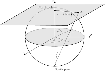
Figure 1: Stereographic projection of the sphere onto the plane.

2.2 Mother spherical wavelets

Admissible mother spherical wavelets may be constructed from the stereographic projection of admissible mother Euclidean wavelets on the plane:

$$\psi(\omega)=[\Pi^{-1}\psi_{\mathbb{R}^{2}}](\omega)\>.$$ (6)

Directional spherical wavelets may be naturally constructed in this setting – they are simply the projection of directional Euclidean planar wavelets on to the sphere.

We consider three spherical wavelets in our subsequent cross-correlation analysis: the spherical Mexican hat wavelet (SMHW); the spherical butterfly wavelet (SBW); and the spherical real Morlet wavelet (SMW). These spherical wavelets are illustrated in Fig. 2. Each spherical wavelet is constructed by the stereographic projection of the corresponding Euclidean wavelet onto the sphere, where the Euclidean planar wavelets are defined by

$$\psi_{\mathbb{R}^{2}}^{\rm{\rm SMHW}}(r,\phi)=\frac{1}{2}(2-r^{2})\,{\rm e}^{-r^{2}/2}\>,$$

$$\psi_{\mathbb{R}^{2}}^{\rm{\rm SBW}}(x,y)=x\,{\rm e}^{-(x^{2}+y^{2})/2}$$

and

$$\psi_{\mathbb{R}^{2}}^{\rm{\rm SMW}}(\mathbf{x};\mathbf{k})={\rm Re}\left({\rm e}^{\mathit{i}\mathbf{k}\cdot\mathbf{x}/\sqrt{2}}\>{\rm e}^{-\|\mathbf{x}\|^{2}/2}\right)$$

respectively, where $\mathbf{k}$ is the wave vector of the SMW. The SMHW is proportional to the Laplacian of a Gaussian, whereas the SBW is proportional to the first partial derivative of a Gaussian in the $x$-direction. The SMW is a Gaussian modulated sinusoid, or Gabor wavelet.

The dilation parameter of each wavelet may be related to an effective size on the size for the wavelet. For directional wavelets we define two effective sizes on the sky defined in orthogonal directions. The SMHW and SBW are both derived from a parent Gaussian function and thus for each direction have the same effective size on the sky, defined by $\xi^{{\rm SMHW},\,{\rm SBW}}_{i}(c_{i})\approx 2\sqrt{2}\>c_{i}$, where $i=\{1,2\}$ and $c_{i}=\{a,b\}_{i=1,2}$ (McEwen et al., 2005b). The first effective size of the SMW defines the overall size of the wavelet on the sky $\xi^{{\rm SMW}}_{1}(a)\approx 2\sqrt{2}\>a$, whereas the second orthogonal size defines the size of the internal structure of the wavelet $\xi^{{\rm SMW}}_{2}(b)\approx b\pi/k_{0}$ (McEwen et al., 2005b).

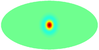
(a) Spherical Mexican hat wavelet (SMHW)

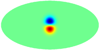
(b) Spherical butterfly wavelet (SBW)

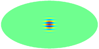
(c) Spherical real Morlet wavelet (SMW)

Figure 2: Spherical wavelets at scale $a=b=0.2$. Wavelet maps are displayed in the Mollweide projection, where the wavelets have been rotated down from the north pole for ease of observation. The SMW is plotted for wave vector $\mathbf{k}=(10,0)^{T}$.

3 Cross-correlation in wavelet space

The effectiveness of using a spherical wavelet estimator to detect cross-correlations between the CMB and the nearby galaxy density distribution has been demonstrated by Vielva et al. (2006). We extend the wavelet estimator here to account for directional wavelets that are not azimuthally symmetric. Firstly, we review the theoretical cross-power spectrum of the CMB and galaxy density and give an expression for the spectrum based on the particular cosmological model. We then define the wavelet coefficient covariance estimator used to test for cross-correlations. Using the theoretical cross-power spectrum previously described, we give a theoretical prediction for the wavelet coefficient covariance for a particular cosmological model (i.e. for a particular theoretical cross-power spectrum). In subsequent sections, we use this result to compare theoretical predictions of the wavelet covariance for a range of cosmologies with measurements from the data, in order to place constraints on the cosmological parameters that define the dark energy. Finally, we also examine in this section the effectiveness of various spherical wavelets for detecting cross-correlations.

3.1 Theoretical cross-power spectrum

For a particular cosmology, we consider the theoretical cross-power spectrum $C_{\ell}^{\rm NT}$ of the galaxy density map $n(\omega)$ with the CMB temperature anisotropy map $t(\omega)$, defined as the ensemble average of the product of the spherical harmonic coefficients of the two maps:

$$\left<n_{\ell m}\>t_{\ell^{\prime}m^{\prime}}^{\ast}\right>=\delta_{\ell\ell^{\prime}}\delta_{mm^{\prime}}\>C_{\ell}^{\rm NT}\>,$$ (7)

where $\delta_{ij}$ is the Kronecker delta function. In defining the cross-correlation in this manner we implicitly assume that the galaxy density and CMB random fields on the sphere are homogeneous and isotropic. Modelling the observation process, the observed cross-spectrum for the given cosmology is related to the theoretical one by

$$C_{\ell}^{\rm NT,obs}=p_{\ell}{}^{2}\>b_{\ell}^{{\rm N}}\>b_{\ell}^{{\rm T}}\>C_{\ell}^{\rm NT}\>,$$ (8)

where $p_{\ell}$ is the pixel window function for the pixelisation scheme adopted and $b_{\ell}^{{\rm N}}$ and $b_{\ell}^{{\rm T}}$ are the beam window functions for the galaxy density and CMB maps respectively. Pixel window and beam functions are represented here by Legendre coefficients (rather than spherical harmonic coefficients).

The theoretical cross-power spectrum may be computed for a given cosmology by (e.g. Nolta et al. 2004)

$$C_{\ell}^{\rm NT}=12\pi\Omega_{\rm m}H_{0}{}^{2}\int\frac{\mathrm{\,d}k}{k^{3}}\>\Delta_{\delta}^{2}(k)\>F_{\ell}^{\rm N}(k)\>F_{\ell}^{\rm T}(k)\>,$$ (9)

where $\Omega_{\rm m}$ is the matter density, $H_{0}$ is the Hubble parameter, $\Delta_{\delta}^{2}(k)=k^{3}P_{\delta}(k)/2\pi^{2}$ is the logarithmic matter power spectrum ($P_{\delta}(k)$ is the matter power spectrum) and $F_{\ell}^{{\rm N}}(k)$ and $F_{\ell}^{{\rm T}}(k)$ are the filter functions for the galaxy density distribution and CMB respectively, given by

$$F_{\ell}^{{\rm N}}(k)=b\int\mathrm{\,d}z\>\frac{\mathrm{\,d}N}{\mathrm{\,d}z}\>D(z)\>j_{\ell}[k\eta(z)]$$ (10)

and

$$F_{\ell}^{{\rm T}}(k)=\int\mathrm{\,d}z\>\frac{\mathrm{\,d}g}{\mathrm{\,d}z}\>j_{\ell}[k\eta(z)]\>.$$ (11)

The integration required to compute $F_{\ell}^{\rm T}(k)$ is performed over $z$ from zero to the epoch of recombination, whereas, in practice, the integration range for $F_{\ell}^{\rm N}(k)$ is defined by the source redshift distribution function $\frac{\mathrm{\,d}N}{\mathrm{\,d}z}$. The function $D(z)$ is the linear growth factor for the matter distribution (calculated from CMBFAST (Seljak & Zaldarriaga, 1996) by computing the transfer function for different redshifts), $g\equiv(1+z)D(z)$ is the linear growth suppression factor, $j_{\ell}[k\eta(z)]$ is the spherical Bessel function and $\eta(z)$ is the conformal look-back time. The bias factor $b$ is assumed to be redshift independent.

For the evolution of $D(z)$ we consider both the standard model dominated by a cosmological constant and also alternative models dominated by a time varying dark energy with negative pressure, $\rho=\rho_{0}(1+z)^{3(1+w)}$, and energy density that is spatially inhomogeneous. These alternative models are parameterised by the equation-of-state parameter $w$, defined as the ratio of pressure to density. The standard inflationary model assumes a homogeneous field (the cosmological constant) with $w=-1$, however in general dark energy models are characterised by values of $w<0$. For instance, topological defects can be phenomenologically represented by an equation-of-state parameter $-2/3\leq w\leq-1/3$ (e.g. Friedland et al. 2003), quintessence models imply $-1<w<0$ (Wetterich, 1988; Caldwell et al., 1998) and phantom models have equation-of-state parameter $w<-1$ (these last models, however, violate the null dominant energy condition; see Carroll et al. (2003) for a detailed discussion).

A convincing explanation for the origin and nature of the dark energy within the framework of particle physics is lacking, nevertheless in general the models considered in the literature produce a $w$ that varies with time. For most dark energy models, however, the equation-of-state changes slowly with time and a standard approximation is that (at least during a given epoch) $w$ can be considered as a constant equation-of-state parameter (Wang et al., 2000). Henceforth, we consider $w$ to be constant as a useful approach to extract fundamental properties of the dark energy.

3.2 Wavelet covariance estimator

The covariance of the wavelet coefficients is used as an estimator to detect any cross-correlation between the CMB and the galaxy density distribution. A positive covariance indicates a positive cross-correlation between the data. The wavelet coefficient covariance estimator is defined as the sum over all points on the wavelet domain sky, of the product of the wavelet coefficient maps:

$$\hat{X}_{\psi}^{{\rm N}{\rm T}}({a,b},\gamma)=\frac{1}{N_{\alpha\beta}}\sum_{\alpha,\beta}\>\nu_{\alpha\beta}\>{W}_{\psi}^{\rm N}({a,b},\alpha,\beta,\gamma)\>{W}_{\psi}^{\rm T}({a,b},\alpha,\beta,\gamma)\>,$$ (12)

where $N_{\alpha\beta}$ is the number of samples in the wavelet domain sky, $\nu_{\alpha\beta}$ is a weighting function and ${W}_{\psi}^{\rm N}({a,b},\alpha,\beta,\gamma)$ and ${W}_{\psi}^{\rm T}({a,b},\alpha,\beta,\gamma)$ are the wavelet coefficients of the galaxy density distribution and CMB respectively. We choose weights to reflect the relative size of the pixels on the sky in the wavelet domain (equiangular sampling is used in the wavelet coefficient Euler angle domain), where $\nu_{\alpha\beta}=\frac{\pi}{2}\sin\beta$. This weighting scheme ensures regions near the poles of the coordinate system do not have a greater influence on the estimated covariance than regions near the equator.

We may also average the covariance estimator over orientations, so that we obtain an overall covariance measure for the given scales:

$$\hat{X}_{\psi}^{{\rm N}{\rm T}}({a,b})=\frac{1}{N_{\gamma}}\sum_{\gamma}\>\hat{X}_{\psi}^{{\rm N}{\rm T}}({a,b},\gamma)\>,$$ (13)

where $N_{\gamma}$ is the number of samples in the wavelet domain orientational component. This measure is still sensitive to directional structure when using a directional spherical wavelet, just as $\hat{X}_{\psi}^{{\rm N}{\rm T}}({a,b},\gamma)$ and $\hat{X}_{\psi}^{{\rm N}{\rm T}}({a,b})$ are both sensitive to localised spatial structure in $(\alpha,\beta)$.

A theoretical prediction of the wavelet covariance may be specified for a given cosmological model. Vielva et al. (2006) derive this for azimuthally symmetric spherical wavelets, however the extension to directional wavelets is non-trivial. We present the derivation of the theoretical wavelet covariance for directional wavelets in Appendix A, stating here the expression for the theoretical covariance obtained:

$$X_{\psi}^{{\rm N}{\rm T}}({a,b},\gamma)=\sum_{\ell=0}^{\infty}\>p_{\ell}{}^{2}\>b_{\ell}^{{\rm N}}\>b_{\ell}^{{\rm T}}\>C_{\ell}^{\rm NT}\sum_{m=-\ell}^{\ell}\left|(\psi_{{a,b}})_{\ell m}\right|^{2}\>,$$ (14)

where $\psi_{\ell m}$ are the spherical harmonic coefficients of the wavelet. In practice at least one of the functions in (14) has a finite band limit so that negligible power is present in those coefficients above a certain ${\ell_{\rm max}}$. All summations over $\ell$, here and subsequently, may therefore be truncated to ${\ell_{\rm max}}$.

3.3 Comparison of wavelet covariance estimators

We compare the expected performance of various spherical wavelets for detecting the ISW effect in this section. Vielva et al. (2006) perform a similar analysis to compare the performance of the SMHW estimator to real and harmonic space estimators, showing the effectiveness of the SMHW estimator. Instead we focus here on comparing wavelets; thus we extend the analysis to directional wavelets.

The expected signal-to-noise ratio (${\rm SNR}$) of the wavelet covariance estimator of the CMB and the LSS density distribution may be used to compare the expected performance of various wavelets for detecting the ISW effect. The expected ${\rm SNR}$ for a particular scale is given by the ratio of the expected value of the wavelet covariance estimator and its dispersion:

$${\rm SNR}_{\psi}({a,b})=\frac{\left<\hat{X}_{\psi}^{{\rm N}{\rm T}}({a,b})\right>}{\Delta\hat{X}_{\psi}^{{\rm N}{\rm T}}({a,b})}\>,$$ (15)

where for a directional wavelet the variance of the wavelet covariance estimator is given by

$$\left[\Delta\hat{X}_{\psi}^{{\rm N}{\rm T}}({a,b})\right]^{2} = \left<\left[\hat{X}_{\psi}^{{\rm N}{\rm T}}({a,b})\right]^{2}\right>-\left<\hat{X}_{\psi}^{{\rm N}{\rm T}}({a,b})\right>^{2}$$ (16)

$$= \displaystyle\sum_{\ell=0}^{\infty}\frac{1}{2\ell+1}\>p_{\ell}{}^{4}\>(b_{\ell}^{{\rm N}})^{2}\>(b_{\ell}^{{\rm T}})^{2}\>$$

$$\times\>\left(\sum_{m=-\ell}^{\ell}\left|(\psi_{{a,b}})_{\ell m}\right|^{2}\right)^{2}\left((C_{\ell}^{\rm NT})^{2}+C_{\ell}^{\rm TT}C_{\ell}^{\rm NN}\right)\,,$$

where $C_{\ell}^{\rm TT}$ and $C_{\ell}^{\rm NN}$ are the CMB and galaxy count power spectra respectively. For the case of azimuthally symmetric wavelets (16) reduces to the form given by Vielva et al. (2006).

The expected ${\rm SNR}$ is computed for the spherical wavelets we consider for a range of dilations (the dilations considered are those that are subsequently used to attempt to detect the ISW effect, as defined in Table 1). The theoretical power spectra used in this experiment are computed from the cosmological concordance model parameters specified in Table 1 of Spergel et al. (2003) ($\Omega_{\Lambda}=0.71$, $\Omega_{\rm m}=0.29$, $\Omega_{\rm b}=0.047$, $H_{0}=72$, $\tau=0.166$, $n=0.99$). CMBFAST is used to simulate the CMB spectrum $C_{\ell}^{\rm TT}$, the cross-power $C_{\ell}^{\rm NT}$ spectrum is simulated in accordance with the theory outlined in section 3.1, while the actual NVSS data is used to provide the LSS angular power spectrum $C_{\ell}^{\rm NN}$. Ideal noise-free and full-sky conditions are assumed for this experiment. Beam and pixel windowing are not considered in the results presented, although when included these factors make only a very minimal difference to the numerical values obtained. The expected ${\rm SNR}$ computed for each wavelet for a range of scales is illustrated in Fig. 3. The relative expected performance of the SMW for detecting the ISW effect is low, thus we do not consider this wavelet any further. The SMHW and the SBW are of comparable expected performance. However, notice that the elliptical SMHW (illustrated by the off-diagonal values of Fig. 3 (b)) and the SBW are slightly superior to the azimuthally symmetric SMHW (illustrated by the diagonal values of Fig. 3 (b)). It may appear counter intuitive initially that asymmetric wavelets may perform better at detecting the ISW effect when the data are isotropic fields. Although the statistics of the fields are globally isotropic, this does not preclude local oriented features in the data. Indeed, the distribution of the ellipticity of peaks in a isotropic Gaussian random field has been derived by Barreiro et al. (1997, 2001), illustrating that one would expect to see local rotationally invariant features. The maximum expected ${\rm SNR}$ achievable with both the SMHW and SBW is approximately 4, compared to an estimated best achievable ${\rm SNR}$ of approximately 7.5 for a perfect survey (Afshordi, 2004).

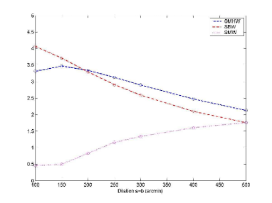
(a) All wavelets for isotropic dilations

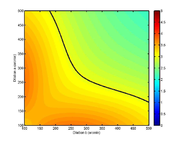
(b) SMHW for all dilations

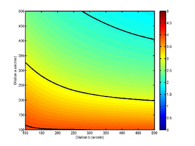
(c) SBW for all dilations

Figure 3: Expected ${\rm SNR}$ of the wavelet covariance estimator of CMB and radio source maps (cosmological parameters are chosen according to the concordance model). All spherical wavelets are considered for isotropic dilations in panel (a): SMHW (blue, dashed); SBW (red, dotted-dashed); SMW (magenta, dotted). Due to the relatively poor expected performance of the SMW, the ${\rm SNR}$ for all anisotropic dilations in only shown for the SMHW and SBW in panels (b) and (c) respectively. Contours at ${\rm SNR}$ values of two, three and four are also plotted in panels (b) and (c).

4 Analysis procedure

We describe in this section the data and an overview of the analysis procedure used to attempt to detect the ISW effect using directional spherical wavelets.

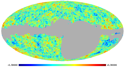
(a) WMAP

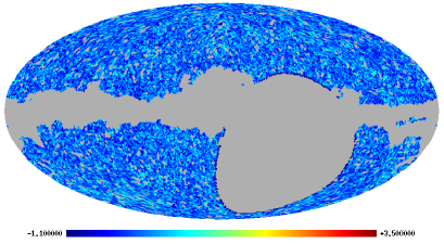
(b) NVSS

Figure 4: WMAP and NVSS maps after application of the joint mask. The maps are represented in the HEALPix format at a resolution of $N_{\rm side}=64$ (corresponding to a pixel size of $\sim\!\!55\arcmin$).

4.1 WMAP data

To minimise the contribution of foregrounds and systematics to CMB anisotropy measurements the WMAP assembly contains a number of receivers that observe at a range of frequencies. The WMAP team and other independent groups have proposed various constructions of CMB maps from data measured by different receivers and bands in order to minimise foreground contributions (template based methods: Bennett et al. 2003b; template independent methods: Bennett et al. 2003b, Tegmark et al. 2003, Eriksen et al. 2004). In this work, we use the template based foreground removed maps (Bennett et al., 2003b) to construct the co-added map proposed by the WMAP team and used in their non-Gaussianity analysis (Komatsu et al., 2003). Following the data processing pipeline specified by Komatsu et al. (2003), the foreground cleaned WMAP maps for which the CMB is the dominant signal (two Q-band maps at 40.7GHz, two V-band maps at 60.8GHz and four W-band maps at 93.5GHz) are combined to give the signal-to-noise ratio enhanced co-added map. The conservative Kp0 exclusion mask provided by the WMAP team is applied to remove remaining Galactic emission and bright point sources. The foreground removed maps used to construct the co-added map and the Kp0 mask are available from the Legacy Archive for Microwave Background Data Analysis (LAMBDA). The maps are provided in the HEALPix (Górski et al., 2005) format at a resolution of $N_{\rm side}=512$ (giving $12N_{\rm side}{}^{2}\sim 3\times 10^{6}$ pixels on the sphere). Since the ISW signal we hope to detect is expected to be generated by structure on scales greater than $2^{\circ}$ (Afshordi, 2004), we down-sample the co-added map constructed to $N_{\rm side}=64$ ($\sim 5\times 10^{4}$ pixels). This corresponds to a pixel size of approximately $55\arcmin$ and so should be of sufficient resolution to detect the ISW signal. The co-added WMAP map used in the subsequent analysis is displayed in Fig. 4 (a) (with the joint Kp0-NVSS mask applied, as described in section 4.2).

4.2 NVSS data

We use the NVSS radio source catalogue as a local tracer of the LSS. The catalogue covers approximately 80% of the sky and contains measurements of almost $2\times 10^{6}$ point sources with a minimum flux density of $\sim\!\!2.5$mJy. Although the distance of individual sources is largely unknown, the sources are thought to be distributed in the redshift range $0<z<2$ with a peak in the distribution at $z\sim 0.8$ (Boughn & Crittenden, 2002). The ISW signal we hope to detect is expected to be produced at $z\sim 0.4$ with negligible contribution from $z>1.5$ (Afshordi, 2004). Furthermore, the correlations induced by the ISW effect are a relatively large scale phenomenon, hence any detection will be cosmic variance limited. The near full-sky coverage and source distribution of the NVSS data thus make it an ideal probe of the local matter distribution to use when searching for the ISW effect. Indeed, the NVSS catalogue has been used to make positive detections of the ISW effect already using the real space correlation function (Boughn & Crittenden, 2002, 2004; Nolta et al., 2004).

As first noticed by Boughn & Crittenden (2002), the NVSS catalogue mean source density varies with declination. We correct this systematic by scaling each iso-latitude band to impose a constant mean density. The iso-latitude bands are defined by the continuous root-mean-squared (RMS) noise regions of the survey (see Fig. 10 of Condon et al. 1998). Alternative correction strategies were also considered (e.g. the one proposed by Nolta et al. 2004), however we found cross-correlation detections to be insensitive to the particular correction procedure.

We represent the corrected NVSS source distribution in the HEALPix format at the same resolution of the WMAP data ($N_{\rm side}=64$). We consider only the sources in the NVSS catalogue above 2.5mJy, corresponding to an identification completeness of 50% (Condon et al., 1998). No observations are made in the NVSS catalogue for equatorial declination $\delta$ lower than $-50^{\circ}$ and the coverage in the range $-50^{\circ}<\delta<-37^{\circ}$ is not sufficient. Hence, we consider only sources with an equatorial declination $\delta\geq-37^{\circ}$. With these constraints we obtain a galaxy distribution map containing $\sim\!\!1.6\times 10^{6}$ sources with an average number of $40.4$ counts per pixel. Since the WMAP mask and NVSS coverage each exclude various sections of the sky, we construct a joint mask (Kp0$\>+\>\delta\!<\!-37^{\circ}$) that leaves only those common pixels that remain in both maps. This mask is applied to both the co-added WMAP and NVSS maps used in the subsequent analysis. The NVSS map with the joint map applied is displayed in Fig. 4 (b).

4.3 Simulations

Monte Carlo simulations are performed to construct significance measures for the wavelet covariance statistics used to detect the ISW effect. 1000 Gaussian simulations of the WMAP data are constructed from the power spectrum produced by CMBFAST using the cosmological concordance model parameters specified in Table 1 of Spergel et al. (2003). For each realisation we simulate the WMAP observing strategy and then construct a simulated co-added map. Measurements made by the Q-, V- and W-band receivers are simulated by convolving with realistic beams and adding anisotropic WMAP noise for each receiver. The procedure described in section 4.1 to construct the co-added map is then performed on the simulated data. The simulated co-added map is then down-sampled to $N_{\rm side}=64$ and the joint mask is applied.

4.4 Procedure

The analysis procedure consists of computing the wavelet covariance estimator described in section 3.2 from the wavelet coefficients of the co-added WMAP and NVSS data computed for a range of scales and, for the directional wavelets, a range of $\gamma$ orientations. We consider only those scales where the ISW signal is expected to be significant (Afshordi, 2004): the wavelet scales considered and the corresponding effective size on the sky of the wavelets are shown in Table 1. Each of the directional wavelets considered are rotationally invariant under integer azimuthal rotations of $\pi$, thus the azimuthal rotation angle $\gamma$ effectively lies in the domain $[0,\pi)$. For directional wavelets we consider five evenly spaced $\gamma$ orientations in the domain $[0,\pi)$. Any deviation from zero in the wavelet covariance estimator for any particular scale or orientation is an indication of a correlation between the WMAP and NVSS data and hence a possible detection of the ISW effect. An identical analysis is performed using the simulated co-added CMB maps in place of the WMAP data in order to construct significance measures for any detections made. Finally, we use any detections of the ISW effect to constrain dark energy parameters.

The application of the joint Kp0-NVSS mask distorts wavelet coefficients corresponding to wavelets with support that overlaps the mask exclusion region. These contaminated wavelet coefficients must be removed from the wavelet covariance estimate. We construct an extended coefficient mask for each scale to remove all contaminated wavelet coefficients from the analysis. Binary morphological operations, commonly applied on the plane in image processing (Gonzalez, 2003), are extended to the sphere and applied to construct the extended coefficient mask. A morphological dilation adds pixels to the boundaries of regions, whereas a morphological erosion removes pixels from boundaries. Firstly, the original joint mask is ‘opened’ (a morphological dilation followed by an erosion) to remove point source regions whilst maintaining the size of the original central masked region. The central masked region is then extended by half the effective size of the wavelet (at the particular scale) by performing a morphological erosion. The original point source mask regions are then replaced by applying the original mask (point source regions are removed initially to ensure that they are not expanded when performing the final erosion). The result of this procedure is to extend the central region of the joint mask by half the effective size of the wavelet, while maintaining the point source regions. This ensures that all coefficients corresponding to wavelets that overlap with the masked Galactic plane are excluded from the analysis. However, wavelets that overlap with masked point sources are not removed. Retaining these wavelet coefficients induces minimal distortion due to the large support of the wavelets relative to the size of the masked point sources. This is a less conservative procedure for constructing extended coefficient masks than used in our non-Gaussianity analysis (McEwen et al., 2005b), however the low resolution of the data and the large initial joint mask reduce drastically the number of pixels available initially. If we construct more conservative extended masks we find that we quickly and significantly reduce the number of pixels considered and thus the efficiency of the analysis. To ensure any correlations detected are not due to contamination that is not excluded by the extended mask we have also performed a number of tests using masks with larger exclusion regions. We find that the correlation signals that we subsequently detect (see section 5) remain when using these larger exclusion masks. Hence our choice of mask appears appropriate as it is more efficient than more conservative masks but still removes the contaminated wavelet coefficients.

Table 1: Wavelet scales considered in attempting to detect the ISW effect. The effective sizes on the sky of the various wavelets for each wavelet scale are also shown. Note that for anisotropic dilations the wavelets have two effective sizes on the sky defined in orthogonal directions (see text).

Scale	1	2	3	4	5	6	7
Dilation $a$	100′	150′	200′	250′	300′	400′	500′
Size on sky $\xi^{{\rm SMHW},\,{\rm SBW}}_{1,2}(a)=\xi^{\rm SMW}_{1}(a)$	282′	424′	565′	706′	847′	1130′	1410′
Size on sky $\xi^{\rm SMW}_{2}(a)$	31.4′	47.1′	62.8′	78.5′	94.2′	126′	157′

5 Results and discussion

In this section we describe the results obtained when performing the directional spherical wavelet analysis procedure described previously. We describe the detections of the ISW effect that we make, before using the detections to constrain dark energy parameters.

5.1 Detection of the ISW effect

Firstly, we describe the detection of positive correlations between the WMAP and NVSS data using various wavelets. To examine the source of the correlation detected we perform some preliminary tests to ascertain whether perhaps foregrounds or systematics are responsible. We then localise regions on the sky that contribute most strongly to the correlation signal and examine these in more detail.

5.1.1 Detections

The wavelet covariance of the WMAP-NVSS data are shown in Fig. 5 for each of the wavelets considered. The covariance values are shown in units of $N_{\sigma}$, the number of standard deviations that the data measurement differs from the mean of 1000 Monte Carlo simulations for each covariance statistic. On examining the distribution of the wavelet covariance statistics of the simulations, the covariance statistics themselves appear to approximately Gaussian distributed. This implies that the approximate significance of any detection of a non-zero covariance can be inferred directly from the $N_{\sigma}$ level. In any case, 68%, 95% and 99% significance regions are plotted in Fig. 5 also (these significance levels are computed from the simulations directly but correspond approximately to 1.00$\sigma$, 1.96$\sigma$ and 2.57$\sigma$ respectively). The left panel in Fig. 5 shows the results for the azimuthally symmetric SMHW (with isotropic dilations), whereas the other panels correspond to directional wavelets. These latter panels exhibit a jagged structure due to the ordering of the wavelet scale index the covariance is plotted against. The wavelet scale index is ordered by sequentially concatenating rows from the 2-dimensional $({a,b})$ dilation space. It would be preferable to view the data as a surface in $({a,b})$ space, however it would not be possible to view the data and the six significance level surfaces at once. The scale index $j$ used in Fig. 5 and subsequently may be related to the scale index defined in Table 1 for $a$ and $b$ by $\lfloor(j-1)/7\rfloor$ and ${\rm mod}(j-1,7)+1$ respectively, where $\lfloor x\rfloor$ is the largest integer less than $x$ and ${\rm mod}(\cdot,n)$ is the modulo $n$ function. For all of the wavelets considered, the wavelet covariance of the data lies outside of the 99% significance level on certain scales.

   

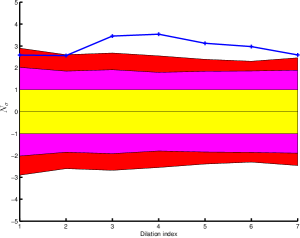
(a) Symmetric SMHW

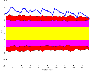
(b) Elliptical SMHW

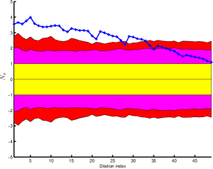
(c) SBW

Figure 5: Wavelet covariance statistics in units of $N_{\sigma}$ for the WMAP and NVSS data against wavelet scale index. Significance levels obtained from 1000 Monte Carlo simulations are shown by the shaded regions for 68% (yellow/light-grey), 95% (magenta/grey) and 99% (red/dark-grey) levels. See text for a discussion of the ordering of the dilation index.

In Fig. 6 we show the $N_{\sigma}$ surfaces for each wavelet in $({a,b})$ space. The maximum $N_{\sigma}$ of all detections made with the directional SMHW and SBW is 3.9 for both wavelets (the maximum detection made with the SBW is slightly greater than that made with the SMHW, however to one decimal place they are equivalent). Using the symmetric SMHW (i.e. using only isotropic dilations) however, one obtains a maximum $N_{\sigma}$ of 3.6. It should be noted that the use of the maximum $N_{\sigma}$ to characterise the detection is based on an a posteriori scale selection: the significance of the detection is characterised for a specific scale, rather than the range of scales examined. It is interesting to note that for both wavelets the $N_{\sigma}$ surfaces displayed in Fig. 6 are perfectly consistent with the expected ${\rm SNR}$ displayed in Fig. 3: the most significant detections are made on scales with high expected ${\rm SNR}$. Note that the $N_{\sigma}$ surface for the SMHW (Fig. 6 (a)) is not perfectly symmetric about the line $a=b$. Although the wavelet has identical shape for dilations $(a,b)$ and $(b,a)$, the second wavelet is rotated azimuthally by $\pi/2$ relative to the first wavelet. Since the starting position differs between the two cases the directional analysis of each probes slightly different directions, resulting in an $N_{\sigma}$ surface that is not perfectly symmetric about the diagonal.

The symmetric SMHW analysis has already been performed by Vielva et al. (2006). We have repeated the analysis here as a consistency check for our analysis and also to confirm the previous work. The wavelet covariance curve shown in Fig. 5 (a) is similar to the curve obtained by Vielva et al. (2006), however we make a slightly more significant detection at $3.6\sigma$ compared to the detection made by Vielva et al. (2006) at $3.3\sigma$. After performing numerous tests with different weighting and masking schemes we believe the difference in significance with Vielva et al. (2006) is due to the different mask construction techniques adopted, the different pixelisation of the wavelet domain and the slightly different definition of the SMHW used (see Martínez-González et al. (2002) for the definition used by Vielva et al. (2006)).

In summary, we have detected a positive correlation between the WMAP and NVSS data, as indicated by a positive wavelet covariance, at the $3.9\sigma$ level on wavelet scales about $(a,b)=(100\arcmin,300\arcmin)$. The sign of the correlation detected (positive) and the scale the detections are made at is consistent with an ISW signal. We next perform some preliminary tests to determine whether the correlation we detect is indeed produced by the ISW effect or whether other factors are responsible.

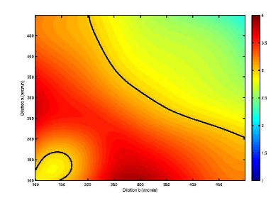
(a) SMHW

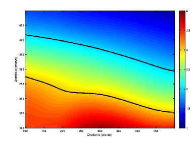
(b) SBW

Figure 6: Wavelet covariance $N_{\sigma}$ surfaces. Contours are shown for levels of two and three $N_{\sigma}$.

5.1.2 Foregrounds and systematics

To test whether foregrounds or WMAP systematics are responsible for the correlation signal we examine the wavelet covariance obtained using both the separate WMAP bands and also combinations of difference maps constructed from the individual bands. We have two Q-band maps at 40.7GHz, two V-band maps at 60.8GHz and four W-band maps at 93.5GHz to construct test maps from (we subsequently use the notation Q1, Q2, etc. to denote the signal measured by each receiver and the single band letter to denote the sum of all maps measured for the given band, e.g. Q=Q1+Q2). Firstly, the wavelet covariance of the NVSS map with each of the Q-, V- and W-band maps is computed and is displayed in Fig. 7. For each case the wavelet covariance signal is essentially identical to the signal observed when using the co-added WMAP map (which is also plotted in Fig. 7 for comparison). Secondly, we construct the difference maps Q1-Q2, V1-V2 and W1-W2+W3-W4 for each band from the signals measured by different receivers. The CMB signal and foreground contributions are completely removed from these noisy difference maps. In addition, we examine the difference map W-V-Q which is free of CMB but has a clear foreground contribution. The wavelet covariance of the NVSS map with each of these difference maps is computed and is displayed in Fig. 8. For all of these difference maps the correlation previously detected in the co-added WMAP is eliminated.

Any correlation between the WMAP and NVSS maps due to unremoved foreground emission in the WMAP data is expected to be frequency dependent, reflecting the emission law of the point source population (e.g. Toffolatti et al. 1998). However we observe identical wavelet covariance signals in each band (Fig. 7) and do not detect any frequency dependence. Furthermore, the W-V-Q difference map has minimal CMB contribution but has a clear foreground contribution. We do not detect any correlation using this map (Fig. 8). These findings suggest that the correlation signal that we detect in the co-added WMAP map is not due to unremoved foregrounds in the WMAP data (we show also in section 5.1.3 that the detection is not due to a few localised regions, giving further evidence to support the claim that unremoved foregrounds are not responsible).

The wavelet covariance signal that we detect in the co-added WMAP map is present in all of the individual WMAP bands (Fig. 7). Furthermore, the covariance signal is eliminated in each of the individual band difference maps that contain no CMB or foreground contributions (Fig. 8). Since all of the WMAP receivers produce an identical covariance signal that does not appear to be due to the noise artifacts of each receiver, we may conclude that it is unlikely that systematics are responsible for the detection made.

These preliminary tests show that it is unlikely that unremoved foreground emission or systematic effects in the WMAP data are responsible for the detection of a positive correlation between the WMAP and NVSS data. It would appear that the detection is due to solely the CMB contribution of the WMAP data. This gives further support to the claim that the correlation we observe is produced by the ISW effect.

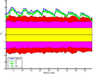
(a) SMHW

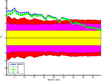
(b) SBW

Figure 7: Wavelet covariance statistics in units of $N_{\sigma}$ computed for the NVSS map with individual WMAP band maps.

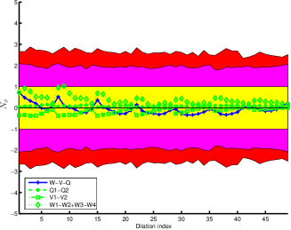
(a) SMHW

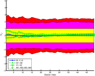
(b) SBW

Figure 8: Wavelet covariance statistics in units of $N_{\sigma}$ computed for the NVSS map with WMAP band difference maps.

5.1.3 Localised regions

A wavelet analysis inherently allows the spatial localisation of interesting signal characteristics. The regions that contribute most strongly to the wavelet covariance detected may therefore be localised, not only in scale, but also in position and orientation on the sky.

The wavelet covariance statistic is essentially the weighted mean of the wavelet domain product map constructed from the product of the WMAP and NVSS wavelet coefficients. The regions that contribute most strongly to the covariance may thus be localised by thresholding the wavelet domain product map. In Fig. 9 we illustrate the localised regions detected once the wavelet product map is thresholded so that only those values that lie above $3\sigma$ remain. For illustrational purposes we show for each wavelet only the localised maps corresponding to the scale and first orientation of the most significant covariance detection. In the subsequent analysis all orientations are considered, thus Fig. 9 is illustrative rather than representing all of the localised regions that we detect. Notice that the localised regions found are relatively evenly distributed over the sky (remember that we cannot search within the extended joint WMAP-NVSS mask, which becomes progressively larger on larger wavelet scales). The localised maps found with the various wavelets also exhibit a fair degree of similarity.

A interesting next step is to determine whether these localised regions are the sole source of the wavelet covariance signal detected. To examine this hypothesis we remove the localised regions detected on all scales and orientations (not just the ones corresponding to the maximum detections that are displayed in Fig. 9) and repeat the analysis. The wavelet covariance signals measured with and without the localised regions removed are shown in Fig. 10. Once the localised regions are removed the covariance signal is reduced in significance, as one would expect since those regions that contribute most strongly are removed, but the covariance signal is not eliminated. Indeed, the signal remains on certain scales at almost the 95% significance level. We conclude that the localised regions that we detect are not the sole source of correlation between the WMAP and NVSS data. Our findings are consistent intuitively with the predicitions of the ISW effect, namely that we would expect any observed correlation to be due to weak correlations over the entire sky rather than a few localised regions. Furthermore, the aggregate nature of the signal detected provides further evidence to suggest that foreground contamination in the data is not responsible. Boughn & Crittenden (2005) make similar conclusions that the correlation signal they detect is due to aggregate correlations over the entire sky rather than a few localised regions.

As a final test of the integrity of the data we examine in more detail a few of the most significant localised regions that we detect. We examine 18 of the localised regions illustrated in Fig. 9, selected from the regions that contain the greatest wavelet coefficient product map values, in both the NVSS and Bonn 1420MHz (Reich, 1982; Reich & Reich, 1986) radio surveys (the latter data set affords better visualisation of the LSS and enables one to highlight regions in the NVSS data for closer examination). The regions selected are defined in Table 2 and Fig. 11. We do not notice any difference in the NVSS data between our localised regions and regions selected at random. The localised regions we detect do not, in general, correspond to regions with particularly bright point sources that could have caused contamination of the data.

All of the tests that we have performed indicate that the correlation detected is indeed due to the ISW effect and not due to systematics or foreground contamination. Next we use our positive detection of the ISW effect to place constraints on dark energy.

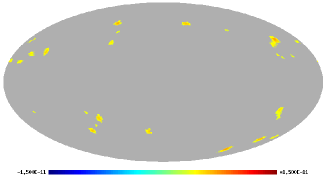
(a) Symmetric SMHW; dilation $({a,b})=(250\arcmin,250\arcmin)$

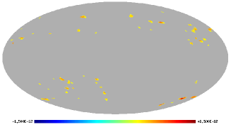
(b) Elliptical SMHW; dilation $({a,b})=(100\arcmin,300\arcmin)$

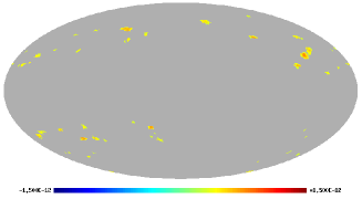
(c) SBW; dilation $({a,b})=(100\arcmin,300\arcmin)$

Figure 9: Localised WMAP-NVSS wavelet coefficient product maps thresholded at $3\sigma$. The regions remaining show those areas that contribute most strongly to the positive wavelet covariance signal detected. Localised product maps are only shown for the first orientation for the scale of the most significant correlation detection made with each wavelet.

   

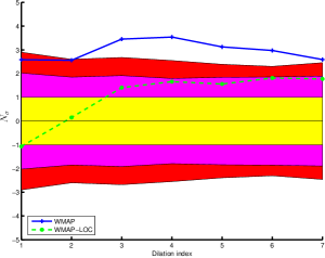
(a) Symmetric SMHW

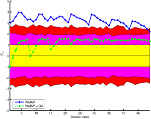
(b) Elliptical SMHW

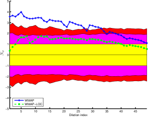
(c) SBW

Figure 10: Wavelet covariance statistics computed for the WMAP and NVSS data with (green/light-grey dots) and without (blue/dark-grey pluses) the localised regions that contribute most strongly to the covariance removed. The covariance signal is reduced in significance when the localised regions are removed, as one would expect, but it is certainly not eliminated suggesting that the localised regions are not the sole source of the wavelet covariance.

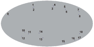
Figure 11: Approximate localised regions flagged for closer examination (see Table 2 for more details).

Table 2: Approximate localised regions flagged for closer examination (see Fig. 11 for a map of these regions). The wavelets that flag each region are listed also (the same regions are flagged by both the symmetric and elliptical SMHW). Although these regions are specified precisely they represent only the approximate position of the regions localised by the wavelet analysis, which is often of the order of a number of degrees.

Region	Location		Flagged by wavelet
	Longitude	Latitude	SMHW	SBW
1	75∘	57∘	$\checkmark$	$\times$
2	75∘	53∘	$\times$	$\checkmark$
3	323∘	56∘	$\checkmark$	$\times$
4	321∘	62∘	$\times$	$\checkmark$
5	267∘	50∘	$\checkmark$	$\times$
6	268∘	45∘	$\times$	$\checkmark$
7	213∘	40∘	$\checkmark$	$\times$
8	223∘	30∘	$\times$	$\checkmark$
9	160∘	26∘	$\checkmark$	$\checkmark$
10	94∘	-28∘	$\checkmark$	$\times$
11	81∘	-34∘	$\checkmark$	$\times$
12	118∘	-42∘	$\times$	$\checkmark$
13	20∘	-48∘	$\checkmark$	$\times$
14	34∘	-31∘	$\times$	$\checkmark$
15	230∘	-68∘	$\checkmark$	$\times$
16	204∘	-56∘	$\checkmark$	$\checkmark$
17	186∘	-54∘	$\checkmark$	$\checkmark$
18	218∘	-33∘	$\checkmark$	$\times$

5.2 Constraints on $\Omega_{\Lambda}$ and $w$

In a flat universe the ISW effect is present only in the presence of dark energy. We may therefore use our detection of the ISW effect to constrain dark energy parameters by comparing the theoretically predicted wavelet covariance signal for different cosmological models with that measured from the data. In particular, we constrain the vacuum energy density $\Omega_{\Lambda}$ and the equation-of-state parameter $w$ (assuming the equation-of-state parameter does not evolve with redshift within the epoch of interest). We probe the parameter ranges $0<\Omega_{\Lambda}<0.95$ and $-2<w<0$. For the other cosmological parameters we use the concordance model values (Spergel et al., 2003). We use a bias parameter value of $b=1.6$. This is the best choice consistent with the concordance model that is within the range favoured by the NVSS data (Boughn & Crittenden, 2002, 2004) when adopting the RLF1 model proposed by Dunlop & Peacock (1990). In any case, Vielva et al. (2006) find dark energy constraints to be insensitive to changes in the bias within the range $1.4<b<1.8$. We also use the Dunlop & Peacock (1990) RLF1 model to describe the $\frac{\mathrm{\,d}N}{\mathrm{\,d}z}$ distribution since it fits the NVSS galaxy autocorrelation function well, as previously shown by Boughn & Crittenden (2002, 2004) and Nolta et al. (2004).

To compare the wavelet covariance of the data with the theoretical predictions made by different cosmological models we compute the $\chi^{2}$ for parameters $\Theta=(\Omega_{\Lambda},w)$, defined by

$$\chi^{2}(\Theta)=\left[\mathbf{X}_{\psi}^{{\rm N}{\rm T}}(\Theta)-\hat{\mathbf{X}}_{\psi}^{{\rm N}{\rm T}}\right]^{\rm T}{\rm C}^{-1}\left[\mathbf{X}_{\psi}^{{\rm N}{\rm T}}(\Theta)-\hat{\mathbf{X}}_{\psi}^{{\rm N}{\rm T}}\right]\>,$$ (17)

where $\mathbf{X}_{\psi}^{{\rm N}{\rm T}}(\Theta)$ is the predicted covariance vector for the given cosmological model and $\hat{\mathbf{X}}_{\psi}^{{\rm N}{\rm T}}$ is the wavelet covariance vector of the data. These vectors are constructed by concatenating the wavelet covariance values computed for the considered dilations and orientations into vectors. The matrix ${\rm C}$ is a similarly ordered covariance matrix of the wavelet covariance statistics, computed from the 1000 Monte Carlo simulations. Making a Gaussian approximation for the likelihood, we may write the likelihood function as $\mathcal{L}(\Theta)\propto\exp\left[-\chi^{2}(\Theta)/2\right]$. The likelihood surfaces for the parameter ranges discussed for both of the SMHW and the SBW are illustrated in Fig. 12. Marginalised likelihood distributions are also shown. Parameter estimates are made from the mean of the marginalised distributions, with 68%, 95% and 99% confidence regions constructed to ensure the required probability is met in the tails of the distribution. The parameter estimates and errors made with the various wavelets are as follows: $\Omega_{\Lambda}=0.63_{-0.17}^{+0.18}$, $w=-0.77_{-0.36}^{+0.35}$ using the SMHW; $\Omega_{\Lambda}=0.52_{-0.20}^{+0.20}$, $w=-0.73_{-0.46}^{+0.42}$ using the SBW. Within error bounds these parameter estimates are consistent with one another and also with estimates made from numerous other analysis procedures and data sets. The errors we obtain on the parameter estimates are relatively large. Although wavelets perform very well when attempting to detect the ISW effect since one may probe different scales, positions and orientations, once all information is incorporated to compute the likelihood surface the performance of a wavelet analysis is comparable to other linear techniques, as expected (see Vielva et al. (2006) for a detailed discussion and comparison of real, harmonic and (azimuthally symmetric) wavelet space techniques for detecting correlations due to the ISW effect).

     

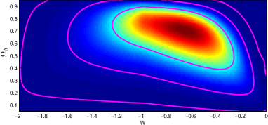
(a) Full likelihood surface obtained using SMHW

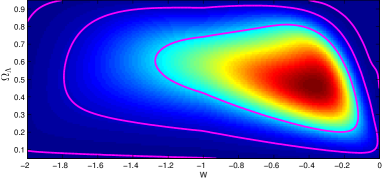
(b) Full likelihood surface obtained using SBW

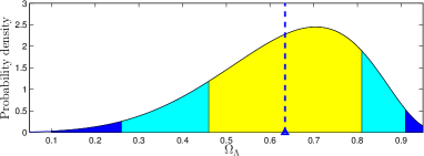
(c) Marginalised distribution for $\Omega_{\Lambda}$ obtained using SMHW

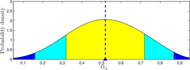
(d) Marginalised distribution for $\Omega_{\Lambda}$ obtained using SBW

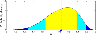
(e) Marginalised distribution for $w$ obtained using SMHW

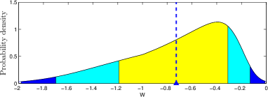
(f) Marginalised distribution for $w$ obtained using SBW

Figure 12: Likelihood surfaces for parameters $\Theta=(\Omega_{\Lambda},w)$. The full likelihood surfaces are shown in the top row of panels, with 68%, 95% and 99% confidence contours also shown. Marginalised distributions for each parameter are shown in the remaining panels, with 68% (yellow/light-grey), 95% (light-blue/grey) and 99% (dark-blue/dark-grey) confidence regions also shown. The parameter estimates made from the mean of the marginalised distribution is shown by the triangle and dashed line.

5.3 Constraints on $\Omega_{\Lambda}$

It is also interesting to use our detection of the ISW effect to provide an estimate of the overall evidence for the existence of dark energy when assuming a pure cosmological constant. We compute the likelihood distribution of just the vacuum energy density $\Omega_{\Lambda}$ in the presence of a cosmological constant by repeating the procedure described in section 5.2 for $\Theta=\Omega_{\Lambda}$ and $w=-1$. This essentially reduces to taking a slice through the 2-dimensional likelihood surfaces shown in Fig. 12 at $w=-1$. The corresponding likelihood distributions for each wavelet are shown in Fig. 13. From the mean of the distributions we obtain the following vacuum energy density estimates: $\Omega_{\Lambda}=0.70_{-0.15}^{+0.15}$ using the SMHW; $\Omega_{\Lambda}=0.57_{-0.18}^{+0.18}$ using the SBW. Within error bounds these parameter estimates are again consistent with each other and with estimates made using other techniques and data sets.

We show also in Fig. 13 the cumulative probability $P(\Omega_{\Lambda}>x)$. One may read directly off this plot the evidence for the existence of dark energy above a certain level. For instance, using the SMHW we may state that $\Omega_{\Lambda}>0.1$ at the $99.96\%$ level. Using the SBW we may state that $\Omega_{\Lambda}>0.1$ at the $99.71\%$ level. The cummulative probability function falls off faster for the SBW, indicating that the SMHW happens to be more effective at ruling out a low vacuum energy density (i.e. the SMHW predicts a higher $\Omega_{\Lambda}$). In any case, we have very strong evidence for dark energy in the case of a pure cosmological constant.

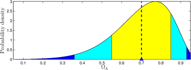
(a) Likelihood distribution for $\Omega_{\Lambda}$ obtained using SMHW

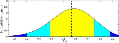
(b) Likelihood distribution for $\Omega_{\Lambda}$ obtained using SBW

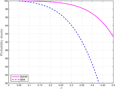
(c) Cumulative probability functions for $P(\Omega_{\Lambda}>x)$

Figure 13: Likelihood distributions and cumulative probability functions for $\Omega_{\Lambda}$ when $w=-1$. Confidence regions at 68% (yellow/light-grey), 95% (light-blue/grey) and 99% (dark-blue/dark-grey) are also shown on the likelihood distributions, with the parameter estimates made from the mean of the distribution shown by the triangle and dashed line. The cummulative probability functions show the probability $P(\Omega_{\Lambda}>x)$ for the SMHW (solid magenta curve) and SBW (dashed blue curve).

6 Conclusions

We have performed a directional spherical wavelet analysis to search for correlations between the WMAP and NVSS data arising from the ISW effect. Wavelets are an ideal tool for searching for the ISW effect due to the localised nature of the effect and the localisation afforded by a wavelet analysis. Furthermore, we use directional spherical wavelets that allow one to probe not only scale and spatially localised structure but also orientated structure in the data.

Using this technique we have detected a significant correlation between the WMAP and NVSS data. The detection is made using both the directional SMHW and the SBW, on approximately the same wavelet scale of $(a,b)=(100\arcmin,300\arcmin)$, corresponding to an overall effective size on the sky of approximately $10{{}^{\circ}}$. The scale and positive sign of the detected correlation is consistent with the ISW effect. To test this hypothesis further we examined other possible causes of the signal and after performing some preliminary tests ruled out both foreground contamination and systematics in the WMAP data. A wavelet analysis inherently provides localised information, thus we were able to localise those regions on the sky that contribute most strongly to the overall correlation. On removing these regions from the analysis the correlation originally detected is reduced in significance, as one would expect, but it is not eliminated, remaining at the 95% significance level in some cases. It therefore appears that although the localised regions that we detected are a strong source of correlation, they are not the sole source. This is again consistent with predictions made using the ISW effect, where one would expect to observe weak correlations over the entire sky rather than just a few localised regions. Finally, we examined 18 of the most significant localised regions in more detail in high-resolution maps of the NVSS and Bonn 1420MHz radio surveys. These regions are not atypical and do not, in general, correspond to regions with particularly bright point sources that could have caused contamination of the data. All of these findings suggest that the correlation that we have detected is due to the ISW effect. In our (nearly) flat universe the ISW effect is present only in the presence of dark energy, hence our detection of the effect is direct evidence for dark energy.

We have used our detection of the ISW effect to constrain dark energy parameters by comparing theoretical predictions made by different cosmological models with the data. Constraining both the vacuum energy density $\Omega_{\Lambda}$ and the equation-of-state parameter $w$, we obtained the following parameter estimates: $\Omega_{\Lambda}=0.63_{-0.17}^{+0.18}$, $w=-0.77_{-0.36}^{+0.35}$ using the SMHW; $\Omega_{\Lambda}=0.52_{-0.20}^{+0.20}$, $w=-0.73_{-0.46}^{+0.42}$ using the SBW. We have therefore obtained independent estimates of the parameters that, within error bounds, are consistent with one another and also with estimates made from many other analysis procedures and data sets. The errors we obtain on the parameter estimates are relatively large. Although wavelets perform very well when attempting to detect the ISW effect since one may probe particular scales, positions and orientations, once all information is incorporated when computing the parameter estimates the performance of the wavelet analysis is comparable to other linear techniques, as expected. We also constrain $\Omega_{\Lambda}$ for the case of a pure cosmological constant, i.e. $w=-1$. For this case we obtain the following parameter estimates: $\Omega_{\Lambda}=0.70_{-0.15}^{+0.15}$ using the SMHW; $\Omega_{\Lambda}=0.57_{-0.18}^{+0.18}$ using the SBW. Again the estimates are consistent with one another and with those made elsewhere. For this case we also examined the evidence for a non-zero cosmological constant, ruling out $\Omega_{\Lambda}<0.1$ at greater than the 99% level using each wavelet.

In this work we have extended to directional wavelets the spherical wavelet analysis technique used to probe CMB data and LSS tracers for cross-correlations. The effectiveness of the wavelet analysis technique is illustrated herein by the highly significant detection of the ISW effect that we are able to make using the WMAP and NVSS data. In addition, the spherical wavelet covariance approach to detecting correlations can be applied to other applications, such as searching for the Sunyaev-Zel’dovich effect (Hansen et al., 2005) or looking for common structures between the CMB and foregrounds (Liu & Zhang, 2006). It would also be interesting to repeat our analysis using different tracers of the LSS and also the next release of the WMAP data to see if the ISW signal that we have detected remains.

Appendix A Theoretical directional spherical wavelet covariance

When using azimuthally symmetric wavelets the spherical harmonic coefficients of the spherical wavelet transform may simply be written as the product of the signal and wavelet harmonic coefficients. This is not the case when using directional wavelets (i.e. wavelets that are not azimuthally symmetric). For this reason the theoretical form of the azimuthally symmetric wavelet covariance estimator derived by Vielva et al. (2006) is not trivially extended to directional wavelets. We derive here the theoretical directional spherical wavelet covariance. For simplicity, and without loss of generality, we ignore beam and pixel window functions in the analysis (which, in any case, may easily be put in by hand at the end if required).

Firstly, we derive an expression for the real space angular correlation function:

$$<n(\omega)\>t^{\ast}(\omega^{\prime})> = \sum_{\ell=0}^{\infty}C_{\ell}^{\rm NT}\>\sum_{m=-\ell}^{\ell}Y_{\ell m}({\omega})\>Y_{\ell m}^{\ast}({\omega^{\prime}})$$ (18)

$$= \sum_{\ell=0}^{\infty}\frac{2\ell+1}{4\pi}\>P_{{\ell}}({\omega\cdot\omega^{\prime}})\>C_{\ell}^{\rm NT}\>,$$

where we have made use of (7) and also the addition theorem for spherical harmonics:

$$\sum_{m=-\ell}^{\ell}Y_{\ell m}({\omega})\>Y_{\ell m}^{\ast}({\omega^{\prime}})=\frac{2\ell+1}{4\pi}\>P_{{\ell}}({\omega\cdot\omega^{\prime}})\>,$$ (19)

where $Y_{\ell m}({\omega})$ are the spherical harmonic functions and $P_{{\ell}}({x})$ are the Legendre polynomials.

Using (18) we may write the theoretical wavelet covariance as

$$<{W}_{\psi}^{\rm N}({a,b},\mathbf{\rho})\>{W}_{\psi}^{{\rm T}\ast}({a,b},\mathbf{\rho})>$$ (20)

$$= \int_{{S^{2}}}\int_{{S^{2}}}\mathrm{\,d}\Omega(\omega)\mathrm{\,d}\Omega(\omega^{\prime})\>\psi_{{a,b},\mathbf{\rho}}^{\ast}(\omega)\>\psi_{{a,b},\mathbf{\rho}}(\omega^{\prime})\>$$

$$\>\>\>\times\><n(\omega)\>t^{\ast}(\omega^{\prime})>$$

$$= \sum_{\ell=0}^{\infty}\frac{2\ell+1}{4\pi}\>C_{\ell}^{\rm NT}\int_{{S^{2}}}\int_{{S^{2}}}\mathrm{\,d}\Omega(\omega)\mathrm{\,d}\Omega(\omega^{\prime})\>$$

$$\>\>\>\times\>\psi_{{a,b},\mathbf{\rho}}^{\ast}(\omega)\>\psi_{{a,b},\mathbf{\rho}}(\omega^{\prime})\>P_{{\ell}}({\omega\cdot\omega^{\prime}})\>.$$

Assuming ergodicity, we may relate (20) directly to our wavelet covariance estimator. Furthermore, under our assumption that both the CMB and galaxy density fields are isotropic, the wavelet covariance is independent of our choice of the position and orientation of the wavelet, hence we may set the rotation of the wavelet to zero, i.e. $\mathbf{\rho}=\mathbf{0}$. Thus we may write

$$X_{\psi}^{{\rm N}{\rm T}}({a,b},\gamma)=\sum_{\ell=0}^{\infty}\frac{2\ell+1}{4\pi}\>C_{\ell}^{\rm NT}\int_{{S^{2}}}\mathrm{\,d}\Omega(\omega)\>G^{\ell}(\omega)\>\psi_{{a,b}}^{\ast}(\omega)$$ (21)

where

$$G^{\ell}(\omega)=\int_{{S^{2}}}\mathrm{\,d}\Omega(\omega^{\prime})\>P_{{\ell}}({\omega\cdot\omega^{\prime}})\>\psi_{{a,b}}(\omega^{\prime})\>.$$ (22)

Notice that the theoretical wavelet covariance specified by (21) is independent of the orientation of the analysis $\gamma$. The assumption of isotropy does not imply that the fields considered cannot contain localised anisotropic structure, thus individual wavelet covariance estimators obtained from the data will vary over orientations, but the theoretical prediction for each orientation will be the same when we consider the statistics of the aggregate fields. Essentially, we get a number of samples of a statistic for which we have a single theoretical prediction, thereby actually increasing the performance of any subsequent comparison between the data and theoretical predictions. Directional wavelets are therefore still advantageous in probing localised oriented structure in the data.

Now we consider the spherical harmonic coefficients of $G^{\ell}(\omega)$. Since $P_{{\ell}}({\omega\cdot\omega^{\prime}})$ is azimuthally symmetric it should be possible to write the spherical harmonic coefficients of $G^{\ell}(\omega)$ simply in terms of the harmonic coefficients of the wavelet:

$$G^{\ell}_{\ell^{\prime}m^{\prime}} = \int_{{S^{2}}}\mathrm{\,d}\Omega(\omega)\>G^{\ell}(\omega)\>Y_{\ell^{\prime}m^{\prime}}^{\ast}({\omega})$$ (23)

$$= \sum_{\ell^{\prime\prime}=0}^{\infty}\>\sum_{m^{\prime\prime}=-\ell^{\prime\prime}}^{\ell^{\prime\prime}}(\psi_{{a,b}})_{\ell^{\prime\prime}m^{\prime\prime}}\>I_{\ell^{\prime\prime}\ell^{\prime}m^{\prime\prime}m^{\prime}}^{\ell}\>,$$

where

$$I_{\ell^{\prime\prime}\ell^{\prime}m^{\prime\prime}m^{\prime}}^{\ell} = \int_{{S^{2}}}\int_{{S^{2}}}\mathrm{\,d}\Omega(\omega)\>\mathrm{\,d}\Omega(\omega^{\prime})\>P_{{\ell}}({\omega\cdot\omega^{\prime}})\>Y_{\ell^{\prime}m^{\prime}}^{\ast}({\omega})\>Y_{\ell^{\prime\prime}m^{\prime\prime}}({\omega^{\prime}})$$ (24)

$$= \int_{{S^{2}}}\int_{{S^{2}}}\mathrm{\,d}\Omega(\omega)\>\mathrm{\,d}\Omega(\omega^{\prime})\>\frac{4\pi}{2\ell+1}$$

$$\>\>\>\times\>\sum_{m=-\ell}^{\ell}Y_{\ell m}({\omega})\>Y_{\ell m}^{\ast}({\omega^{\prime}})\>Y_{\ell^{\prime}m^{\prime}}^{\ast}({\omega})\>Y_{\ell^{\prime\prime}m^{\prime\prime}}({\omega^{\prime}})$$

$$= \frac{4\pi}{2\ell+1}\>\delta_{\ell\ell^{\prime}}\delta_{\ell\ell^{\prime\prime}}\delta_{m^{\prime}m^{\prime\prime}}\>,$$

where we make use of the addition theorem for spherical harmonics again. The last line follows from the orthogonality of the spherical harmonics:

$$\int_{{S^{2}}}\mathrm{\,d}\Omega(\omega)\>Y_{\ell m}({\omega})\>Y_{\ell^{\prime}m^{\prime}}({\omega})=\delta_{\ell\ell^{\prime}}\delta_{mm^{\prime}}\>.$$ (25)

Thus, the harmonic coefficients of $G^{\ell}(\omega)$ are given by

$$G^{\ell}_{\ell^{\prime}m^{\prime}}=\frac{4\pi}{2\ell+1}\>(\psi_{{a,b}})_{\ell^{\prime}m^{\prime}}\>\delta_{\ell\ell^{\prime}}\>.$$ (26)

We are now in a position to derive the final expression for the theoretical wavelet covariance in terms of the wavelet spherical harmonic coefficients and the theoretical CMB-galaxy density cross-power spectrum. Expanding $G^{\ell}(\omega)$ in (21) into its spherical harmonic decomposition yields

$$X_{\psi}^{{\rm N}{\rm T}}({a,b},\gamma) = \sum_{\ell=0}^{\infty}C_{\ell}^{\rm NT}\>\sum_{m=-\ell}^{\ell}\>(\psi_{{a,b}})_{\ell m}\int_{{S^{2}}}\mathrm{\,d}\Omega(\omega)\>Y_{\ell m}({\omega})\>\psi_{{a,b}}^{\ast}(\omega)$$ (27)

$$= \sum_{\ell=0}^{\infty}C_{\ell}^{\rm NT}\>\sum_{m=-\ell}^{\ell}\>\left|(\psi_{{a,b}})_{\ell m}\right|^{2}\>,$$

where the last line follows from representing $\psi_{{a,b}}^{\ast}(\omega)$ by its harmonic expansion and noting again the orthogonality of the spherical harmonics (25). For the case of azimuthally symmetric wavelets the $m$-modes of the spherical harmonic coefficients of the wavelet are non-zero only for $m=0$, thus (27) reduces to the form given by Vielva et al. (2006) (the $({2\ell+1})/{4\pi}$ discrepancy arises since Vielva et al. (2006) use Legendre, rather than spherical harmonic coefficients). We have therefore obtained a simple form, that may be computed easily, for the theoretical wavelet covariance of directional wavelets in terms of the wavelet spherical harmonic coefficients and the cross-power spectrum.

References

- Afshordi (2004) Afshordi N., 2004, Phys. Rev. D., 70, 83536
- Afshordi et al. (2004) Afshordi N., Loh Y. -S., Strauss M. A., 2004, Phys. Rev. D., 69, 83524
- Antoine et al. (2004) Antoine J. -P., Murenzi R., Vandergheynst P., Ali S. T., 2004, Two-dimensional wavelets and their relatives, Cambridge University Press, Cambridge
- Antoine & Vandergheynst (1999) Antoine J. -P. and Vandergheynst P., 1999, Applied and Computational Harmonic Analysis, 7, 1
- Antoine & Vandergheynst (1998) Antoine J. -P. and Vandergheynst P., 1998, J. of Math. Phys., 39, 8, 3987
- Antoine et al. (2002) Antoine J. -P., Demanet L., Jacques L., 2002, Applied and Computational Harmonic Analysis, 13, 3, 177
- Barreiro et al. (2000) Barreiro R. B., Hobson M. P., Lasenby A. N., Banday A. J., Górski K. M. and Hinshaw G., 2000, Mon. Not. Roy. Astron. Soc., 318, 475
- Barreiro et al. (2001) Barreiro R. B., Martínez-González E., Sanz J. L., 2001, Mon. Not. Roy. Astron. Soc., 322, 411
- Barreiro et al. (1997) Barreiro R. B., Martínez-González E., Sanz J. L., Cayón L., Silk J., 1997, ApJ, 478, 1
- Bennett et al. (2003a) Bennett C. L. et al. (WMAP team), 2003a, ApJS, 148, 1
- Bennett et al. (2003b) Bennett C. L. et al. (WMAP team), 2003b, ApJS, 148, 97
- Bennett et al. (1996) Bennett C. L., Banday A. J., Górski K. M., Hinshaw G., Jackson P., Keegstra, P., Kogut A., Smoot G. F., Wilkinson D. T., Wright E. L., 1996, ApJ, 464, 1
- Bogdanova et al. (2005) Bogdanova I., Vandergheynst P., Antoine J. -P., Jacques L., Morvidone M., 2005, Applied and Computational Harmonic Analysis, 19, 2, 223
- Boldt (1987) Boldt E., 1987, Phys. Rep., 146, 215
- Boughn & Crittenden (2005) Boughn S. P., Crittenden R. G., 2005, Mon. Not. Roy. Astron. Soc., 360, 1013
- Boughn & Crittenden (2004) Boughn S. P., Crittenden R. G., 2004, Nature, 427, 45
- Boughn & Crittenden (2002) Boughn S. P., Crittenden R. G., 2002, Phys. Rev. Lett., 88, 21302
- Caldwell et al. (1998) Caldwell R. R., Dave R., Steinhardt P. J., 1998, Phys. Rev. Lett., 80, 1582
- Carroll et al. (2003) Carroll S. M., Hoffman M., Trodden M., 2003, Phys. Rev. D., 68, 23509
- Cayón et al. (2005) Cayón L., Jin J., Treaster A., 2005, Mon. Not. Roy. Astron. Soc., 362, 826
- Cayón et al. (2003) Cayón L., Martínez-González E., Argüeso F., Banday A. J., Górski K. M., 2003, Mon. Not. Roy. Astron. Soc., 339, 1189
- Cayón et al. (2001) Cayón L., Sanz J. L., Martínez-González E., Banday A. J., Argüeso F., Gallegos J. E., Górski K. M., Hinshaw G., 2001, Mon. Not. Roy. Astron. Soc., 326, 1243
- Condon et al. (1998) Condon J. J. et al., 1998, ApJ, 115, 1693
- Corasaniti et al. (2005) Corasaniti P. -S., Giannantonio T., Melchiorri A., 2005, Phys. Rev. D., 71, 123521
- Crittenden & Turok (1996) Crittenden R. G., Turok N., 1996, Phys. Rev. Lett., 76, 575
- (26) Cruz M., Tucci M., Martínez-González E., Vielva P., 2006, Mon. Not. Roy. Astron. Soc., 369, 57
- (27) Cruz M., Martínez-González E., Vielva P., Cayón L., 2005, Mon. Not. Roy. Astron. Soc., 356, 29
- Dunlop & Peacock (1990) Dunlop S. J., Peacock J. A., 1990, Mon. Not. Roy. Astron. Soc., 247, 19
- Eriksen et al. (2004) Eriksen H. K., Banday A. J., Górski K. M., Lilje P. B., 2004, ApJ, 612, 633
- Fosalba & Gaztaaga (2004) Fosalba P., Gaztaaga E., 2004., Mon. Not. Roy. Astron. Soc., 350, 37
- Fosalba et al. (2003) Fosalba P. Gaztaaga E., Castander F., 2003, ApJ, 597, 89
- Friedland et al. (2003) Friedland A., Murayama H., Perelstein M., 2003, Phys. Rev. D., 67, 43519
- Gonzalez (2003) Gonzalez R. L., 2001, Digital Image Processing, Second Edition, Prentice Hall
- Górski et al. (2005) Górski K. M., Hivon E., Banday A. J., Wandelt B. D., Hansen F. K., Reinecke M., Bartelmann M., 2005, ApJ, 622, 759
- Hansen et al. (2005) Hansen F. K., Branchini E., Mazzotta P., Cabella P., Dolag K., 2005, Mon. Not. Roy. Astron. Soc., 361, 753
- Hu & Scranton (2004) Hu W., Scranton R., 2004, Phys. Rev. D., 70, 123002
- Jarrett et al. (2000) Jarrett T. H. et al., 2000, ApJ, 119, 2498
- Komatsu et al. (2003) Komatsu E. et al., 2003, ApJS, 148, 119
- Liu & Zhang (2006) Liu X., Zhang S. N., 2006, ApJL, 636, 1
- Liu & Zhang (2005) Liu X., Zhang S. N., 2005, ApJ, 633, 542
- Maddox et al. (1990) Maddox S. J., Efstathiou G., Sutherland W. J., Loveday J., 1990, Mon. Not. Roy. Astron. Soc., 242, 43
- McEwen et al. (2005a) McEwen J. D., Hobson M. P., Mortlock D. J., Lasenby A. N., 2005a, IEEE Trans. Sig. Proc., in press (astro-ph/0506308)
- McEwen et al. (2005b) McEwen J. D., Hobson M. P., Lasenby A. N., Mortlock D. J., 2005b, Mon. Not. Roy. Astron. Soc., 359, 1583
- Martínez-González et al. (2002) Martínez-González E., Gallegos J. E., Argüeso F., Cayón L., Sanz J. L., 2002, Mon. Not. Roy. Astron. Soc., 336, 22
- Mukherjee & Wang (2004) Mukherjee P., Wang Y., 2004, ApJ, 613, 51
- Nolta et al. (2004) Nolta et al. (WMAP team), ApJ, 608, 10
- Padmanabhan et al. (2004) Padmanabhan N., Hirata C. M., Seljak U., Schlegel D. J., Brinkmann J., Schneider D. P., 2004, submitted to Phys. Rev. D., 72, 043525
- Peebles & Ratra (2003) Peebles P. J. E., Ratra B., 2003, Rev. Mon. Phys. 75, 599
- Perlmutter et al. (1999) Perlmitter S. et al. (The Supernova Cosmology Project), 1999, ApJ, 517, 565
- Pogosian et al. (2005) Pogosian L., Corasaniti P. S., Stephan-Otto C., Crittenden R., Nichol R., 2005, Phys. Rev. D., 72, 103519
- Pogosian (2004) Pogosian L., 2004, JCAP, 504, 15
- Reich (1982) Reich W., 1982, A&AS, 48, 219
- Reich & Reich (1986) Reich P., Reich W., 1986, A&AS, 63, 205
- Riess et al. (1998) Riess A. G. et al., 1998, Astron. J., 116, 1009
- Sachs & Wolfe (1967) Sachs R. K., Wolfe A. M., 1967, ApJ, 147, 73
- Scranton et al. (2003) Scranton R. et al. (SDSS collaboration), 2003, submitted to Phys. Rev. Lett. (astro-ph/0307335)
- Seljak & Zaldarriaga (1996) Seljak U., Zaldarriaga M., 1996, ApJ, 469, 437
- Spergel et al. (2003) Spergel D. N. et al. (WMAP team), 2003, ApJS, 148, 175
- Tegmark et al. (2003) Tegmark M., de Oliveira-Costa A., Hamilton A. J. S., 2003, Phys. Rev. D., 68, 12
- Toffolatti et al. (1998) Toffolatti L., Argueso Gomez F., de Zotti G., Mazzei P., Franceschini, A., Danese, L., Burigana, C., 1998, Mon. Not. Roy. Astron. Soc., 297, 117
- Tosic et al. (2005) Tosic I., Frossard P., Vandergheynst P., 2005, Proc. IEEE DCC
- Vielva et al. (2006) Vielva P., Martínez-González E., Tucci M., 2006, Mon. Not. Roy. Astron. Soc., 365, 891
- Vielva et al. (2004) Vielva P., Martínez-González E., Barreiro R. B., Sanz J. L., Cayón L., 2004, ApJ, 609, 22
- Wandelt & Górski (2001) Wandelt B. D., Górski K. M., 2001, Phys. Rev. D., 63, 123002, 1
- Wang et al. (2000) Wang L., Caldwell R. R., Ostriker J. P., Steinhardt P. J., 2000, ApJ, 530, 17
- Wetterich (1988) Wetterich C., 1988, Nucl. Phys. B., 302, 668
- Wiaux et al. (2006) Wiaux Y., Vielva P., Martínez-González E., Vandergheynst P., 2006, Phys. Rev. Lett., 96, 151303
- (68) Wiaux Y., Jacques L., Vandergheynst P., 2005, ApJ, 632, 15
- York et al. (2000) York D. et al. (SDSS collaboration), 2000, Astron. J., 120, 1579