Rotational mixing in low-mass stars

In this paper we study the effects of rotation in low-mass, low-metallicity RGB stars. We present the first evolutionary models taking into account self-consistently the latest prescriptions for the transport of angular momentum by meridional circulation and shear turbulence in stellar interiors as well as the associated mixing processes for chemicals computed from the ZAMS to the upper RGB. We discuss in details the uncertainties associated with the physical description of the rotational mixing and study carefully their effects on the rotation profile, diffusion coefficients, structural evolution, lifetimes and chemical signatures at the stellar surface. We focus in particular on the various assumptions concerning the rotation law in the convective envelope, the initial rotation velocity distribution, the presence of $\mu$-gradients and the treatment of the horizontal and vertical turbulence.

This exploration leads to two main conclusions : (1) After the completion of the first dredge-up, the degree of differential rotation (and hence mixing) is maximised in the case of a differentially rotating convective envelope (i.e., $j_{CE}(r)=cst$), as anticipated in previous studies. (2) Even with this assumption, and contrary to some previous claims, the present treatment for the evolution of the rotation profile and associated meridional circulation and shear turbulence does not lead to enough mixing of chemicals to explain the abundance anomalies in low-metallicity field and globular cluster RGB stars observed around the bump luminosity. This study raises questions that need to be addressed in a near future. These include for example the interaction between rotation and convection and the trigger of additional hydrodynamical instabilities.

1 Abundance anomalies in RGB stars

The standard theory of stellar evolution predicts that the surface chemical composition of low-mass stars is modified on the way to the red giant branch (RGB) during the so-called first dredge-up (hereafter 1st DUP; Iben Iben65 (1965)). There, the expanding stellar convective envelope (hereafter CE) deepens in mass, leading to the dilution of the surface material within regions that have undergone partial hydrogen burning on the earlier main sequence (hereafter MS). Qualitatively, this leads to the decrease of the surface abundances of the fragile LiBeB elements and of ¹²C, while those of ³He, ¹³C and ¹⁴N increase. Abundances of O and heavier elements remain essentially unchanged. Quantitatively, these abundance variations depend on the stellar mass and metallicity (e.g., Sweigart, Greggio & Renzini, Sweigart89 (1989); Charbonnel CC94 (1994); Boothroyd & Sackmann BS99 (1999)). After the 1st DUP, the CE withdraws while the hydrogen burning shell (hereafter HBS) moves outward in mass. Within the standard framework no more variations of the surface abundance pattern are expected until the star reaches the asymptotic giant branch.

Observations sampling the evolution from the turn-off to the base of the RGB in open clusters and in the galactic field stars have validated these predicted surface abundances variations up to the completion of the 1st DUP (e.g. Gratton et al. Gratton00 (2000)). However observational evidence have accumulated of a second and distinct mixing episode which is not predicted by standard models and which occurs in low-mass stars after the end of the 1st DUP, and more precisely at the RGB bump.

The determination of the carbon isotopic ratio ¹²C/¹³C (hereafter CIR) for RGB stars in open clusters with various turn-off masses (Gilroy Gilroy89 (1989)) provided the first pertinent clue on this process. It was indeed shown that bright RGB stars with initial masses lower than $\sim 2-2.5\leavevmode\nobreak\ {\rm M}_{\odot}$ exhibit CIR considerably lower than predicted by standard models after the 1st DUP. Thanks to data collected in stars sampling the RGB of M67 (Gilroy & Brown GB91 (1991)), it clearly appeared that observations deviated from standard predictions just at the so-called RGB bump (Charbonnel CC94 (1994)). The Hipparcos parallaxes allowed to precisely determine the evolutionary phase of large samples of field stars with known CIR. These stars were found to behave similarly as those in M67, e.g. presented unpredicted low CIR appearing at the RGB bump luminosity (Charbonnel, Brown & Wallerstein CBW98 (1998); Gratton et al. Gratton00 (2000)).

On the other hand the region around the bump has also been probed for two globular clusters (GCs). In NGC 6528 and M4 again, the CIR drops below the 1st DUP standard predictions just at the RGB bump (Shetrone 2003a ; 2003b ). Moreover, all the brightest RGB stars observed so far in globular clusters exhibit CIR close to the equilibrium value of the CN cycle.

During this second mixing episode surface abundances of other chemical elements are also affected both in field and GCs giants : Li decreases at the RGB bump (Pilachowski, Sneden & Booth Pila93 (1993); Grundahl et al. Grundahl02 (2002)). C decreases while N increases for RGB stars brighter than the bump (Gratton et al. Gratton00 (2000); Bellman et al. Bellman01 (2001) and references therein), confirming the envelope pollution by CN processing. In the case of GCs, the picture is however blurred by the probable non-negligible dispersion of the initial [C/Fe]. As far as lithium, carbon isotopes and nitrogen are concerned, the abundance variations on the upper RGB have similar amplitudes in field and globular cluster giants (Smith & Martell Smith03 (2003)). The finding that the so-called super Li-rich giants (Wallerstein & Sneden 1982) all lie either at the RGB bump or on the early-AGB (Charbonnel & Balachandran CB00 (2000)), certainly indicates the occurrence of an extra-mixing episode at these evolutionary points. The trigger of this mixing episode has been suggested to be of external nature (Denissenkov & Herwig, (2004)), but is much likely related to the aforementioned second mixing episode, which would start with a Li-rich phase as proposed by Palacios et al. (PCF01 (2001)).

For more than a decade it has been known that in addition to the elements discussed previously, O, Na, Mg and Al also show variations in GC red giants (Kraft et al. Kraft93 (1993); Ivans et al. Ivans99 (1999); Ramirez & Cohen RC02 (2002)). As in the case of lighter nuclei, an in situ mixing mechanism was frequently invoked to explain these abundance anomalies, and in particular the O-Na anti-correlation. For a long time this specific pattern could only be observed in the brightest GC RGB stars. However, O and Na abundances have recently been determined with 8-10m class telescopes in lower RGB and in turn-off stars for a couple of GCs (for recent reviews see Sneden 2005 and Charbonnel 2005 and references therein) revealing exactly the same O-Na anti-correlation as in bright giants. This result is crucial. Indeed, the NeNa-cycle does not operate in MS low-mass stars, as the involved reactions require high temperatures that can only be reached on the RGB. The existence of the same O-Na anti-correlation on the MS and on the RGB in these clusters thus proves that this pattern does not result from self-enrichment. The recent determination of oxygen isotopic ratios in a few RGB stars with low CIR (Balachandran & Carr Bala03 (2003)) reinforces this result. These objects indeed present high ¹⁶O/¹⁷O and ¹⁶O/¹⁸O ratios, in agreement with extensive CN-processing but no dredge-up of ON-cycle material. The O-Na anti-correlation is generally assumed to be of primordial origin, even though it has been proved difficult to find stellar candidates able to produce it (Decressin & Charbonnel, (2005),Denissenkov & Herwig, (2003)). Let us finally mention the peculiar case of M13 bright giants, where O, Na, Mg and Al abundances appear to vary with luminosity. In this cluster the observed O-Na anti-correlation could thus be the result of a superimposition of self-enrichment with a primordial pattern (Johnson05).

In short, observations provide definitive clues on an additional mixing episode occurring in low-mass stars after the end of the 1st DUP. This process appears to be universal and independent of the stellar environment : it affects more than 95$\%$ of low-mass stars (Charbonnel & do Nascimento CdN98 (1998)), whether they belong to the field, to open or globular clusters. Some indications of such a process have also been detected in the brightest RGB stars of external galaxies like the LMC (Smith et al. Smith02 (2002)) and Sculptor (Geisler et al. G05 (2005)). Its signatures in terms of abundance anomalies are clear : the Li and ¹²C abundances as well as the ¹²C/¹³C ratio drop while the ¹⁴N and the ¹⁶O/¹⁸O ratio increase. These data attest the presence of a non-standard mixing process connecting the stellar convective envelope with the external layers of the HBS where CN-burning occurs. Last but not least, they indicate that the effects of this process on surface abundances appear when the star reaches the RGB bump.

Why should the RGB bump be such a special evolutionary point in the present context? After the completion of the 1st DUP, the CE retreats leaving a discontinuity of mean molecular weight (or $\mu$-barrier) at the mass coordinate of its maximum penetration. Subsequently, when the HBS eventually crosses this discontinuity, the star suffers a structural re-adjustment due to the composition changes (more H is made available in the burning shell). The resulting alteration of the energetics causes a momentary decrease of the stellar luminosity. This results in a higher probability for finding a star in this brightness bin, and translates into a bump in the luminosity functions of globular clusters. Standard theory and observations nicely agree on the size and the location of the bump in the HRD (e.g., Zoccali et al. Zocca99 (1999)).
As for mixing in radiative stellar interiors, it was suggested that the discontinuity of molecular weight left by the 1st DUP could inhibit any extra-mixing between the base of the convective envelope and the HBS. After the bump, the $\mu$-gradients are much smoother in this region, permitting some extra-mixing to occur (Sweigart & Mengel SM79 (1979); Charbonnel CC95 (1995); Charbonnel et al. CBW98 (1998)).

2 From the pioneering work on stellar rotation to the present treatment of the transport of angular momentum and chemicals

Sweigart & Mengel (SM79 (1979), hereafter SM79) investigated the possibility that meridional circulation might lead to the mixing of CNO-processed material in RGB stars. Though the physics of rotation-induced mixing invoked at that time was very crude, this pioneering work has magnificently settled the basis of a complex problem. SM79 discussed in great details the problem of $\mu$-gradients which were known to inhibit meridional circulation (Mestel Mestel53 (1953), Mestel57 (1957)). For mixing to be efficient, they underlined the necessity for the radiative zone separating the CE from the HBS not to present significant molecular weight gradients. The other crucial point made by SM79 concerned the importance of the angular momentum (hereafter AM) distribution within the deep CE of RGB stars on the resulting mixing of CNO processed material. Indeed, beyond the 1st DUP, the angular velocity of a radiative layer near the HBS depends sensitively on how much AM has been deposited by the retreating CE. SM79 investigated two extreme cases, namely a constant specific angular momentum and a uniform angular velocity within the CE. Substantial CNO processing of the envelope could be obtained with plausible MS angular velocity only when the inner part of the convection envelope was allowed to depart from solid body rotation. As we shall see in this paper, our lack of knowledge of the distribution of angular momentum within the CE of giant stars remains one of the weakest points of our global understanding of rotation-induced mixing at this phase.

Rotational transport processes cannot be simply reduced to meridional circulation. Once established, this large scale circulation generates advection of AM, and thus favours the development of various hydrodynamical instabilities. Zahn (Zahn92 (1992)) proposed a description of the interaction between meridional circulation and shear turbulence, pushing forward the idea of chocking the meridional circulation by $\mu$-gradients. Following these developments but using a simplified version of Zahn’s description, Charbonnel (CC95 (1995)) re-investigated the influence of such a process in RGB stars. She conjectured that the combination of the disappearance of the mean molecular weight gradient barrier after the bump and the increase of mixing in the HBS has the proper time dependence to account for the observed behaviour of carbon isotopic ratios and for the Li abundances in Population II low-mass giants.

In these exploratory computations however, the diffusion coefficient for chemicals was derived from an assumed constant rotation velocity (in the radiative zone) on the RGB, and the transport of AM by hydrodynamical processes was not considered. This is however of utmost importance in the understanding of the rotation-induced mixing (see the review by Maeder & Meynet MM00araa (2000)).

Then, Denissenkov & Tout (DT00 (2000)) applied the formalism of Maeder & Zahn (MZ98 (1998)) to a typical globular cluster RGB star. However, this was done in a post-processing approach and thus, did not take into account the feedback of mixing on the stellar structure. Considering the angular velocity at the base of the CE as a free adjustable parameter and treating the transport of chemicals only beyond the bump as in the aforementioned works, they obtained large diffusion coefficients able to reproduce not only the Li, C and N abundance anomalies at the bump, but also the O-Na and Mg-Al anti-correlations. These two features being clearly primordial, Denissenkov & VandenBerg (DV03 (2003)) revised these results. They simplified their previous approach, letting AM evolve only due to structural readjustments (no rotational transport), and derived a diffusion coefficient to be applied to the chemicals beyond the bump. They considered the obtained mixing rate to have “the correct order of magnitude”, even though it is too low by a factor of 7 to reproduce the observational data for Pop I stars.

In the present paper we propose a self-consistent approach of rotational-mixing in low-mass RGB stars. We define here as self-consistent a model in which the transport of angular momentum and of chemicals is coupled to the evolution of the star from the zero age main sequence on. If meridional circulation and shear-induced turbulence are the only transport processes of AM considered, the assumptions made on the rotation profile concern solely the initial condition, i.e. the rotation profile at the ZAMS (assumed to be uniform) and the rotation regime in the convective envelope. At each evolutionary step we thus compute the new rotation profile together with the associated transport coefficients resulting from structural readjustments and transport processes associated with rotation. The abundance profile of each chemical is then modified under the effect of both mixing and nuclear reactions. In such a procedure, the stellar structure “reacts” to rotational-mixing.
We discuss the effects of rotation in RGB stars taking into account the latest prescriptions for the transport of AM in stellar interiors, and the associated mixing processes. We describe the physical inputs of our models in § 3 and § 4, and their effects on the angular velocity profiles and diffusion coefficients in § 5. In § 6 we present the results for structural evolution and surface abundance variations of rotating low-mass Pop II stars from the ZAMS to the upper RGB. We then give a summary of our main results, and discuss them in relation with previous works in § 7, and propose new investigation paths in § 8.

3 Physical inputs for the evolution of rotating stars

3.1 Standard input physics

The models presented here were computed with STAREVOL V2.30, and the reader is referred to Siess et al. (Siess2000 (2000)) and Palacios et al. (2003, paper I ) for a detailed description. Let us recall the main inputs.

The nuclear reaction rates have been updated using the version 5.0 of the nuclear network generator NetGen available at IAA (http://astropc0.ulb.ac.be/Netgen). By default the adopted rates are : NACRE (Angulo et al. Ang99 (1999)) for charged particles, Bao et al. (Bao (2000)) for neutron capture rates, Horiguchi et al. (Ho96 (1996)) for experimental beta decay rates and Caughlan & Fowler (CF88 (1988)) otherwise.

For the radiative opacities, we use the OPAL tables above 8000 K (Iglesias & Rogers IR96 (1996)) and at lower temperatures the atomic and molecular opacities of Alexander & Fergusson (Alex (1994)). The conductive opacities are computed from a modified version of the Iben (Iben75 (1975)) fits to the Hubbard & Lampe (Hu69 (1969)) tables for non-relativistic electrons and from Itoh et al. (Ito83 (1983)) and Mitake et al. (Mi84 (1984)) for relativistic electrons.

The equation of state is described in detail in Siess et al. (2000) and accounts for the non ideal effects due to coulomb interactions and pressure ionization. The standard mixing length theory is used to model convection with $\alpha_{\rm MLT}=1.75$ and the atmosphere is treated in the gray approximation and integrated up to an optical depth $\tau\simeq 5\times 10^{-3}$.

3.2 Transport of angular momentum

The evolution of AM and chemical species follow Zahn (Zahn92 (1992)) and Maeder & Zahn (MZ98 (1998)). Meridional circulation and turbulence induced by the secular shear instability are the two transport mechanisms considered here. Within this framework, the transport of AM obeys an advection/diffusion equation

$$\rho\frac{{\rm d}\left(r^{2}\Omega\right)}{{\rm d}t}=\frac{1}{5r^{2}}\frac{\partial}{\partial r}\left(\rho r^{4}\Omega U_{r}\right)+\frac{1}{r^{2}}\frac{\partial}{\partial r}\left(r^{4}\rho\nu_{v}\frac{\partial\Omega}{\partial r}\right),$$ (1)

where $\rho$, $r$ and ${\rm\Omega}$ have their usual meaning. $\nu_{v}$ is the vertical component of the turbulent viscosity associated with the shear instability. $U_{r}$ is the vertical component of the meridional circulation velocity, which, assuming shellular rotation, is given by:

$$U_{r}=\frac{P}{C_{p}\rho Tg[\nabla_{\rm ad}-\nabla+\varphi/\delta\nabla_{\mu}]}\times\left[\frac{L}{M_{*}}(E_{\Omega}+E_{\mu})\right]$$ (2)

where $M_{*}=M(1-\frac{\Omega^{2}}{2\pi G\rho_{m}})$. $E_{\Omega}$ and $E_{\mu}$ depend respectively on the relative horizontal variation of the density, $\Theta=\frac{\tilde{\rho}}{\rho}=\frac{1}{3}\frac{r^{2}}{g}\frac{{\rm d}\Omega^{2}}{{\rm d}r}$, and of the mean molecular weight, $\Lambda=\frac{\tilde{\mu}}{\mu}$. Detailed expressions for these quantities are given in Appendix A. The evolution of $\Lambda$ depends on the competition between the vertical advection of a mean molecular weight gradient $\frac{\partial\ln\overline{\mu}}{\partial r}$ and its destruction by horizontal diffusion $D_{h}$ (see § 3.4)

$$\frac{\partial\Lambda}{\partial t}+U_{r}\frac{\partial\ln\overline{\mu}}{\partial r}=-\frac{6}{r^{2}}D_{h}\Lambda$$ (3)

This equation is obtained under the assumption that

$$\frac{D_{v}}{\ell_{v}^{2}}\ll\frac{D_{h}}{\ell_{h}^{2}}.$$ (4)

$D_{v}$ is the vertical turbulent diffusion coefficient (see § 3.4), $\ell_{v}$ and $\ell_{h}$ are the characteristic distance scales in the vertical and horizontal directions respectively. As in paper I, the transport of AM is computed by solving 5 first order differential equations (Eq. 3 + 4 equations resulting from the splitting of Eq. 1) with a Newton-Raphson relaxation method. The upper boundary condition on $\Lambda$ has however been modified compared to paper I, and we used the continuity equation at the base of the CE rather than assuming $\Lambda=0$.

Effects of $\mu$–currents ($E_{\mu}$ term in Eq. 2) are taken into account consistently from the ZAMS up to the upper RGB.

3.3 Transport of chemicals

In the presence of strong anisotropic turbulence, Chaboyer & Zahn (CZ92 (1992)) showed that the vertical advection of chemicals by a large scale circulation combined with strong horizontal diffusion produces a vertical effective diffusivity $D_{\rm eff}$ (see § 3.4). The vertical transport of a chemical species $i$ of concentration $c_{i}$ can thus be described by a pure diffusion equation:

$$\centering{\rho\frac{{\rm d}{c_{i}}}{{\rm d}t}=\underbrace{\dot{c_{i}}}_{\rm\it nuclear}+\underbrace{\frac{1}{r^{2}}\frac{\partial}{\partial r}\left[r^{2}\rho U_{ip}{c_{i}}\right]}_{\rm\it atomic\leavevmode\nobreak\ diffusion}+\underbrace{\frac{1}{r^{2}}\frac{\partial}{\partial r}\left[r^{2}\rho D_{\rm tot}\frac{\partial{c_{i}}}{\partial r}\right]}_{\rm\it macroscopic\leavevmode\nobreak\ processes}.}\@add@centering$$ (5)

$U_{ip}$ is the atomic diffusion velocity of the element with respect to protons, and $D_{\rm tot}$ is the total macroscopic diffusion coefficient, and is the sum of the effective diffusion coefficient (8) and of the vertical turbulent diffusion coefficient $D_{v}$ (see § 3.4).

The diffusion equation (5) is solved for each of the 53 species considered in the code considering $\dot{c_{i}}=0$ (that is, diffusion and nucleosynthesis are decoupled). Here again, we used a Newton-Raphson method, as for the structure and AM transport equations.

3.4 Diffusion and viscosity

Let us briefly recall the various formulations used for the diffusion coefficients entering Eqs. (1), (3) and (5).

• $\nu_{v}$, $D_{v}$
  As in paper I, we assume that the secular shear instability dominates and that vertical shear eventually becomes turbulent in the radiative stellar interiors due to the low viscosity of the plasma (Zahn Zahn74 (1974)). The development of turbulence is subject to the Reynolds criterion and sets in when

  $$Re=\frac{\nu_{v}}{\nu_{\rm mol}+\nu_{\rm rad}}>Re_{c},$$

  where $\nu_{\rm rad}=\frac{4}{15}\frac{aT^{4}}{\kappa c\rho^{2}}$ is the radiative viscosity, $\nu_{\rm mol}$ is the molecular viscosity and $Re_{c}\simeq 10$ is the critical Reynolds number. The shear instability obeys the Richardson criterion, and according to the classical formulation should set in when

  $$\frac{{\rm d}u}{{\rm d}z}>\frac{N^{2}}{Ri_{c}},$$

  where $Ri_{c}=0.25$ is the critical Richardson number. Here, we rather consider a modified Richardson criterion to take into account radiative losses and/or horizontal diffusion as described below. Several modified criteria have been proposed; in this paper we will compare results obtained with two of them.

  • The first criterion assumes that thermal diffusion reduces the stabilising effect of thermal stratification without affecting the chemical part. It leads to (cf. Maeder & Meynet MM96 (1996)):

    $$D_{v}=\nu_{v}=\frac{8}{5}K_{T}\frac{Ri_{c}(rd\Omega/{\rm d}r)^{2}-N^{2}_{\mu}}{N^{2}_{T}},$$ (6)

    where $N^{2}=N^{2}_{T}+N^{2}_{\mu}$ is the Brunt-Väisäälä frequency and $K_{T}$ is the thermal diffusivity. In this paper we will refer to this prescription as MM96.

  • The second criterion, which we used in paper I, also considers the erosion of the chemical stratification by the large horizontal diffusion (cf. Talon & Zahn TZ97 (1997)):

    $$D_{v}=\nu_{v}=\frac{8}{5}\frac{Ri_{c}(rd\Omega/{\rm d}r)^{2}}{N^{2}_{T}/(K_{T}+D_{h})+N^{2}_{\mu}/D_{h}},$$ (7)

    where $D_{h}$ is the horizontal turbulent viscosity. In this paper we will refer to this prescription as TZ97.

  Let us further note that, due to the lack of a better prescription, we assume $D_{v}=\nu_{v}$.

• $D_{\rm eff}$
  The effective diffusion coefficient solely appears in the transport equation of chemicals. In the approximation of highly anisotropic turbulence, it is the diffusive representation of the effects of meridional circulation (Chaboyer & Zahn CZ92 (1992)), and can be written as follows :

  $$D_{\rm eff}=\frac{|rU_{r}|^{2}}{30D_{h}}$$ (8)

• $\nu_{h}$, $D_{h}$
  The vertical turbulent diffusion coefficient $D_{v}$ as well as the effective diffusion coefficient $D_{\rm eff}$ depend on the horizontal component of the turbulent diffusivity $D_{h}$. No description of this diffusivity can be drawn from first principles, and its expression has to be parametrised. Assuming that the differential rotation on an isobar is small compared to unity, Zahn (Zahn92 (1992)) first proposed the following expression for $\nu_{h}$:

  $$\nu_{h}=\frac{r}{C_{h}}\left|\frac{1}{3\rho r}\frac{{\rm d}(\rho r^{2}U)}{{\rm d}r}-\frac{U}{2}\frac{{\rm d}\ln r^{2}\Omega}{{\rm d}\ln r}\right|\equiv\frac{r}{C_{h}}\left|2V-\alpha U\right|,$$ (9)

  where $C_{h}$ is a free parameter of order 1 which we used in our paper I, $V=\frac{1}{6\rho r}\frac{\rm d}{{\rm d}r}\left(\rho r^{2}U\right)$ is the horizontal component of the meridional velocity and $\alpha=\frac{1}{2}\frac{{\rm d}\ln r^{2}\bar{\Omega}}{{\rm d}\ln r}$. Meanwhile, some improvements have been achieved and more realistic prescriptions for the horizontal shear turbulent diffusivity including a dependence on the rotation rate were derived by Maeder (Maeder03 (2003)) and Mathis et al. (MPZ04 (2004)) :

  $$\nu_{h}=\chi^{\frac{1}{n}}\leavevmode\nobreak\ r\leavevmode\nobreak\ \left(r\leavevmode\nobreak\ \bar{\Omega}(r)\leavevmode\nobreak\ V^{k}\leavevmode\nobreak\ [2V-\alpha U]\right)^{\frac{1}{n}},$$ (10)

  where ($\chi$ ; $n$ ; $k$) = ($\frac{3}{400m\pi}$ ; 3 ; 1) in Maeder’s expression (with $m$ = 1,3 or 5), and ($1.610^{-6}$ ; 2 ; 0) in Mathis et al. (MPZ04 (2004)). In Maeder (Maeder03 (2003)), the horizontal turbulent viscosity $\nu_{h}$ is derived from a comparison between the dissipation rate of turbulent energy by meridional circulation and the viscous dissipation rate, while in Mathis et al. (MPZ04 (2004)), it is derived from Couette-Taylor laboratory experiments (see Richard & Zahn RZ99 (1999)).
  The horizontal turbulent diffusion coefficient $D_{h}$ obtained by Eq. (10) is larger than the one derived from expression Eq. (9), and is more consistent with the shellular rotation hypothesis. In the following, we will compare results obtained with these two prescriptions, which we refer to as $Zahn92$ and $MPZ04$ (see Table 1).

3.5 Rotation law in the convective envelope

The formalism developed by Zahn (Zahn92 (1992)) describes the transport of AM in radiative zones, and the rotation profile in the CE is defined by an upper boundary condition. Its choice is however of prime importance since it determines the flux of angular momentum between these two regions.
In the case of RGB stars, this will play an essential role as discussed in §5.1.

The interaction between rotation and convection is a longstanding and not fully understood problem, and despite the development of 3D numerical simulations (Ballot et al. Ballot04 (2004); Browning et al. Browning04 (2004)), the rotation profile within deep convective envelopes remains unknown. As already suggested by SM79, we may consider two limiting cases for the CE rotation law:

1. Uniform angular velocity (solid body rotation)
   This hypothesis has generally been assumed when modelling the evolution of rotating stars (Endal & Sofia ES78 (1978); Talon et al. TZMM97 (1997); Meynet & Maeder MM00 (2000); paper I). It is also the rotation regime obtained when describing AM transport in the CE by a diffusion equation using the diffusion coefficient derived from the MLT theory (Heger et al. HLW00 (2000)). Imposing solid body rotation in the CE is thus equivalent to assuming that the meridional currents are inhibited in the presence of convection, and that the turbulent viscosity associated with convection is large enough to allow for instantaneous homogenisation of the angular velocity profile $\Omega(r)$, as it is the case for chemicals (Endal & Sofia ES76 (1976)). This condition is also motivated by observations of the solar convection zone (the sole star for which we have such informations at present), where radial differential rotation is minute (Kosovichev et al. kosovichev97 (1997)).

2. Uniform specific angular momentum (differential rotation)
   Already in the early 70’s, Tayler (Tayler73 (1973)) addressed the effects of rotation in stellar convective zones and came to the conclusion that meridional currents could develop and alter the rotation law in stellar convective regions. With caution, he suggested that “it is possible that the asymptotic state [of rotation in a convective zone] is closer to one of uniform angular momentum than uniform angular velocity”. Some years later, Sweigart & Mengel (SM79 (1979)) proposed that rotation-induced mixing by meridional circulation could explain both the CNO abundance anomalies in RGB stars and the slow rotation rates observed in MS low-mass stars provided the radiative interior conserves its angular momentum during the first ascent of the giant branch, and the CE has constant (${\rm d}j_{\rm CE}/{\rm d}t=0$) and uniform (${\rm d}j_{\rm CE}/{\rm d}r={\rm cst}$) specific angular momentum. More recently, Denissenkov & Tout (DT00 (2000)) investigated both possibilities for rotation in the CE of a low-mass RGB star, and concluded in favour of uniform and constant specific angular momentum in the CE. Investigating the rotation rates on horizontal branch (HB) stars of globular clusters, Sills & Pinsonneault (SP00 (2000)) showed that slow rotation on MS stars and $\upsilon\sin i$ up to $40\leavevmode\nobreak\ \>{\rm km}.{\rm s}^{-1}$ on the HB indicate that a non-negligible amount of AM is preserved in the stellar interior between the MS turn-off and the HB. They proposed that this could be achieved assuming uniform specific angular momentum in the CE during the RGB phase, a conclusion again similar to that drawn by SM79 and more recently, by Chanamé et al. (2004a, b).

   These studies indicate that the condition of differential rotation in the CE (i.e. $j_{\rm CE}(r)=\frac{2}{3}r^{2}\Omega(r)={\rm cst}$) could be a key ingredient to derive a consistent history of the AM evolution in low-mass stars, as well as to produce a high degree of mixing in the RGB interiors needed to explain part of the abundance anomalies observed at this phase.

Table 1: Rotation input physics of the models. $D_{h}$ : MPZ04 refers to Mathis et al. (2004) whereas Zahn92 refers to Zahn (1992). $D_{v}$ : TZ97 refers to Talon & Zahn (1997) and MM96 refers to Maeder & Meynet (1996). Uniform specific angular momentum in the CE was only applied beyond the turn-off. All models were computed with uniform angular velocity in the CE during the MS phase. Braking, if applied, begins at the ZAMS following a Kawaler (1988) law calibrated in order to lead to equatorial rotational velocity of $\upsilon\approx 10\>{\rm km}.{\rm s}^{-1}$ when they reach the Hyades age (this occurs for $T_{\rm eff}\approx 6300\leavevmode\nobreak\ {\rm K}$) early on the main sequence. This velocity is typical of cool stars in the Hyades. The highlighted row indicates our reference model M1.

Model	CE	$\upsilon_{\rm ZAMS}$	Braking	$D_{h}$	$\mu$-currents	$D_{v}$
	rotation law	$\>{\rm km}.{\rm s}^{-1}$
M0	—	0	—	—	—	—
M1	$\Omega(r)=$ cst	5	no	MPZ04	yes	TZ97
M2	$j(r)=$ cst	5	no	MPZ04	yes	TZ97
M3	$j(r)=$ cst	5	no	MPZ04	no	TZ97
M4	$j(r)=$ cst	5	no	MPZ04	yes	MM96
M5	$j(r)=$ cst	5	no	Zahn92	yes	TZ97
M6	$j(r)=$ cst	110	yes	MPZ04	yes	TZ97

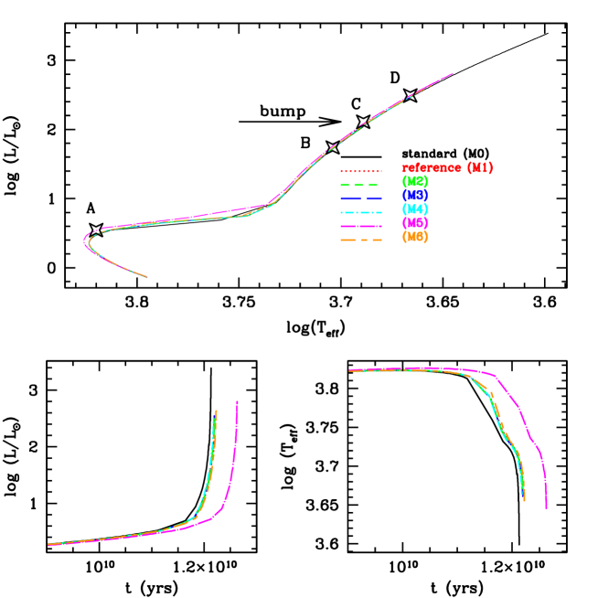
Figure 1:  Upper panel: Hertzsprung-Russell diagram for the different test models presented. All sequences start with $M_{\rm ZAMS}=0.85\,{\rm M}_{\odot}$, [Fe/H] = $-1.57$. Evolutionary tracks for models M1 and M3 are superimposed. Open symbols labelled A, B, C and D correspond to the turn-off, the end of the 1st DUP, the bump and $L=310\,{\rm L}_{\odot}$ respectively. Lower panels: Evolution of luminosity (left) and effective temperature (right) as a function of time beyond the turn-off.

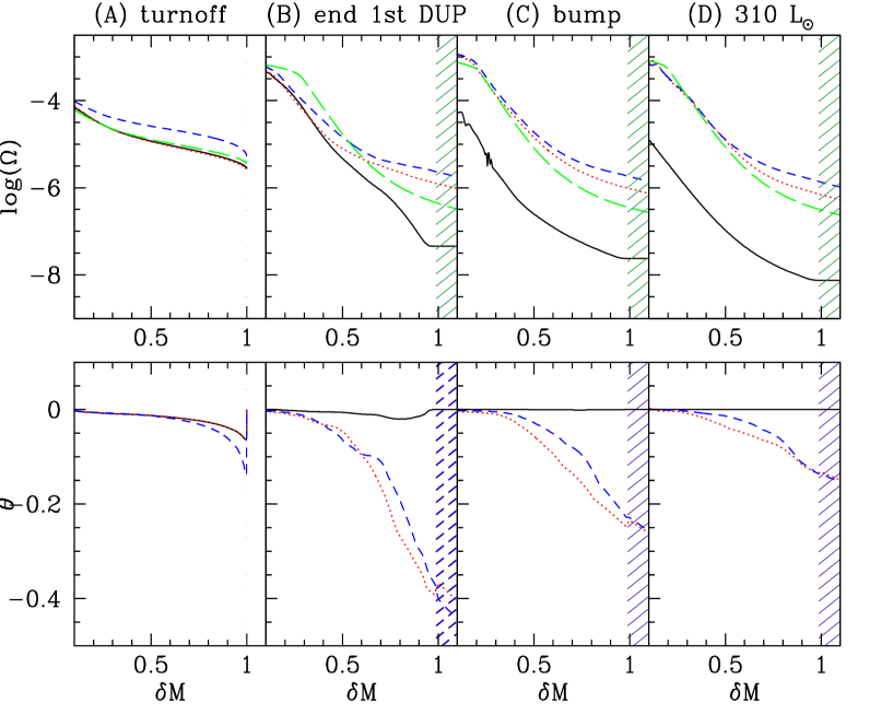
Figure 2: Angular velocity $\Omega$ and horizontal density fluctuations $\theta\propto\partial\Omega/\partial r$ inside models M1 (solid lines), M2 (dotted lines) and M6 (dashed lines) at the four evolutionary points top-labelled on the graph and reported on Fig 1. $\Omega$ and $\theta$ are plotted against the scaled mass coordinate $\delta M$ which allows a blow-up of the region of interest ($\delta M=0$ at the base of the HBS, and $\delta M=1$ at the base of the CE). The long dashed lines on the upper pannels represent the $\Omega$ profiles that one gets when the angular momentum evolution in model M2 only results from the structural readjustments beyond the turn-off (i.e. no AM transport).

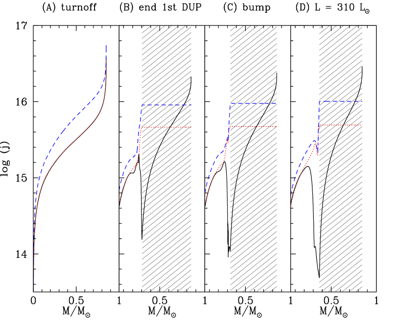
Figure 3: Profile of the logarithm of the specific angular momentum $\log(j)$ inside models M1 (solid lines), M2 (dotted lines) and M6 (dashed lines) at the four evolutionary points top-labelled on the graph and reported on Fig. 1, as a function of the internal mass coordinate $M_{r}$ in units of ${\rm M_{\odot}}$.

4 Numerical simulations

We model a typical metal-poor globular cluster RGB star, with initial mass $M=0.85$ ${\rm M_{\odot}}$, initial helium content $Y_{\rm ini}=0.248$ and $[{\rm Fe/H}]=-1.57$ which corresponds to the metallicity of M13 stars (Sneden et al. SKGPF04 (2004)). We take into account the $\alpha$-enrichment expected at such metallicities, with [O/Fe] = [Ne/Fe] = [Mg/Fe] = $+0.3$ dex, and account for the odd-even effect on sodium, with [Na/Fe] = $-0.3$ dex. The initial ratio for the magnesium isotopes is ${}^{24}{\rm Mg}:^{25}{\rm Mg}:^{26}{\rm Mg}=87.5:6:6.5$, and is similar to the values determined by Yong et al. (Yong03 (2003)) for the stars with the lowest ${}^{25}{\rm Mg}$ and ${}^{26}{\rm Mg}$ in NGC 6752, a globular cluster with [Fe/H]$\approx-1.6$. The mass fractions of the other elements are in solar system proportion, and scaled for their sum to be equal to unity. This corresponds to a metallicity of $Z=8\leavevmode\nobreak\ 10^{-4}$.

Mass loss is included from the ZAMS on in all our models. We use the empirical Reimers (Reimers75 (1975)) formula with a metallicity scaling :

$$\dot{M}=-3.9810^{-13}\eta\frac{L\,R}{M}\sqrt{\frac{Z}{Z_{\odot}}}\leavevmode\nobreak\ \leavevmode\nobreak\ {\rm M}_{\odot}\,{\rm yr}^{-1}$$ (11)

with $\eta=0.5$. At each time step, the associated AM losses are taken into account and the adjusted total AM is conserved when applying rotational transport.

All models are computed assuming uniform angular velocity in the CE during the MS as indicated by the solar case. When considered, the hypothesis of uniform specific angular momentum in the CE is applied beyond the turn-off, i.e. when the convective envelope begins to deepen. We will compare two different rotational histories, namely models that were slow rotators already on the ZAMS and models with an initially larger velocity typical of ZAMS Pop I stars, but which experience magnetic braking in their early evolution, as expected from solar-type stars. This braking results in similar surface velocities at half-way on the main sequence (when $X_{c}\approx 0.5$) for initially fast and slow rotators. Considering their important role in shaping the rotation profile (see paper I), the so-called $\mu$-currents ($E_{\mu}$ term in Eq. 2) are taken into account in all our rotating models except M3. In all cases the initial rotation profile at the ZAMS is defined by $\Omega(r)=\upsilon_{\rm ini}/R_{\star}={\rm cst}\leavevmode\nobreak\ \leavevmode\nobreak\ \forall\leavevmode\nobreak\ \leavevmode\nobreak\ {\rm r}$.

We finally underline that Eq. (1) is solved in all its complexity for all the rotating models presented here from the ZAMS up to the upper RGB.

Table 1 lists the characteristics of the models that we have computed using different prescriptions for the input physics. For our reference model (M1), we consider the following set of parameters/physical ingredients: uniform angular velocity in the convective regions at all times, initial surface velocity of 5 $\>{\rm km}.{\rm s}^{-1}$ on the ZAMS and no braking applied, Mathis et al. (MPZ04 (2004) ; Eq. 10) and Talon & Zahn (TZ97 (1997) ; Eq. 7) prescriptions for the horizontal $\nu_{h}$ and vertical $\nu_{v}$ turbulent diffusion coefficients respectively.

Figure 1 presents the Hertzsprung-Russell diagram and the evolution of the surface luminosity and temperature for the models computed. It will be discussed in more details in § 6.1. The evolutionary points on which we will focus in the following sections are marked on the evolutionary path and correspond to the turn-off (A), the end of the first DUP (B), the bump (C) and $L=310\,{\rm L}_{\odot}$ (D).

5 Testing the physics of rotation

In this section, we analyse the impact of the different physical inputs included in the models presented in Table 1.

5.1 Rotation in the convective envelope

In § 3.5 we mentioned the uncertainty regarding the rotation law in the convective envelope of a giant star. Previous studies also provide some hints that the evolution of the AM (and chemicals) distribution within the radiative interior might strongly depend on the rotation regime at the base of the convective envelope. This aspect can be studied by comparing models M1 and M2, which solely differ by the applied rotation law in the CE beyond the turn-off.

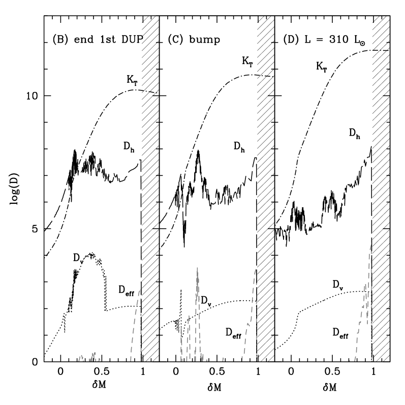
Figure 4: Profiles of the different diffusion coefficients at the end of the first dredge-up (left panel) and at the bump (right panel) for our reference model (M1 in Table 1).

Profiles of the angular velocity $\Omega$, of the horizontal density fluctuations $\theta$ ( = $\frac{\Theta}{\Omega}=\frac{1}{3}\frac{r^{2}}{g}\partial\Omega/\partial r$) and of the specific angular momentum $j$ at four different evolutionary stages for models M1, M2 and M6 are presented in Figs. 2 and 3. In Fig. 2, as well as in several other figures in this paper, quantities are plotted against $\delta M$ instead of $M_{r}$. $\delta M$ is a relative mass coordinate allowing for a blow-up of the radiative region above the HBS, and is defined as

$$\delta M=\frac{M_{r}-M_{\rm HBS}}{M_{\rm BCE}-M_{\rm HBS}}.$$ (12)

$\delta M$ is equal to 1 at the base of the convective envelope and 0 at the base of the HBS (where $X=10^{-7}$). Typically in our models, the nuclear reactions occur between $\delta M$ = 0.2 and $\delta M$ = 0.5, a large mean molecular gradient being associated with the layers of maximum energy production at $\delta M$ = 0.2

By assumption, the rotational evolution is identical in models M1 and M2 up to the turn-off. Beyond, the evolution of the AM distribution is dominated by structural readjustments of the star becoming a giant. The degree of differential rotation in the radiative zone globally increases with time, leading to a rapidly rotating core and a slowly rotating surface ($\Omega$ rises by 3 to 4 orders of magnitude between the base of the CE and the edge of the degenerate He core in both models).
At the turn-off, the base of the CE rotates at the same velocity in models M1 and M2. As the star crosses the Hertzsprung gap and approaches the Hayashi line on its way to the red giant branch, the core contracts while the outer layers expand and are thus efficiently slowed down. For model M1, the velocity of the inner shells of the envelope also decreases substantially because of the solid body rotation of the CE (${\rm d}\Omega_{CE}/{\rm d}r=0$), and the AM attached to the convective envelope concentrates in the outer layers. At the end of the 1st DUP the angular velocity at the base of the CE, $\Omega_{BCE}$, decreased by a factor of 65. When the CE withdraws in mass, it leaves behind radiative shells with low specific angular momentum that rotate slowly. The resulting differential rotation rate is low in this region as shown in the $\theta$ and $\Omega$ profiles.

For model M2, during the 1st DUP the surface layers slow down but the uniformity of the specific angular momentum prevents the shells of the inner CE from decelerating abruptly and ensures the concentration of AM in this denser region. At the end of the 1st DUP, $\Omega_{BCE}$ has decreased only by a factor of 3. As the CE withdraws in mass, its deeper shells retaining the larger part of the CE angular momentum fall back into the underlying radiative zone, where they conserve their large angular velocity and strong differential rotation.

Figure 3 shows that after the completion of the 1st DUP, the assumption of uniform specific angular momentum within the CE also translates into a quasi-constancy of the level of specific angular momentum in this region (dotted and dashed lines in panels (B), (C) and (D)). This is a natural expectation since the convective envelope of a red giant represents more than 80 % of the stellar radius and retains most of the angular momentum. The assumption of constancy of $j_{CE}$ under a regime of uniform specific angular momentum remains however an approximation since transfer of AM occurs between the interior and the envelope. Our models indicate that the specific angular momentum in the envelope indeed slightly increases with time.

The difference of the rotation profiles encountered in models M1 and M2 below the CE affects the diffusion coefficients, in particular $D_{v}$, which scales as $(r{\rm d}\Omega/{\rm d}r)^{2}$.

Figures 4 and 5 present the profiles of the diffusion coefficients entering the transport equations of AM and chemicals (Eqs. 1 and 5) at the end of the 1st DUP, at the bump and at $L=310\,\>{\rm L_{\odot}}$ for models M1 and M2, respectively. One may notice that $D_{h}$ is everywhere much larger than $D_{v}$ (see also Figs. 6, 8 and 9). This validates the shellular rotation hypothesis.

• Model M1
  At the end of the 1st DUP (left panel in Fig. 4), differential rotation is negligible below the CE in the region between $\delta M\simeq 0.5$ and $\delta M$ = 0.91. There, the vertical turbulent viscosity is smaller than its critical value given by $\nu_{v,\rm crit}=Re_{c}\nu_{\rm rad}\simeq 3000$, and turbulence does not develop. The low rate of differential rotation quenches the turbulent transport and creates a gap that disconnects the CE from the regions where nucleosynthesis occurs. Below $\delta M$ $\simeq 0.5$ the differential rotation is larger and the shear turbulence dominates the transport down to the region ($\delta M\approx 0.1$) where both meridional circulation and shear turbulence are very efficiently hindered by the high mean molecular weight barrier associated with the hydrogen burning (see upper panels of Fig. 10). At the bump and beyond, shear-induced turbulence does not develop and the effective diffusion coefficient remains negligible below $\delta M\simeq 0.85$, so that no modification of the surface abundance pattern by rotational mixing should be expected beyond this point (see § 6.2).

• Model M2
  When assuming uniform specific angular momentum in the CE, the picture is very different (Fig. 5). The larger differential rotation rate allows the shear flow to become turbulent almost everywhere between the base of the CE and the HBS. Shear turbulence dominates the transport of chemicals across the entire radiative zone, the effective diffusion coefficient associated with meridional circulation being always much smaller in the whole radiative region. Anticipating the results of § 6.2, we can already see from Fig. 10 that $D_{\rm tot}$ does not rise above $10^{5}{\rm cm}^{2}.{\rm s}^{-1}$ in the outer HBS (around $\delta M$ = 0.2-0.3) even at the bump, which is much lower than the parametric “canonical mixing rate” of $4.10^{8}{\rm cm}^{2}.{\rm s}^{-1}$ deduced from observational constraints (Denissenkov & VandenBerg DV03 (2003)).

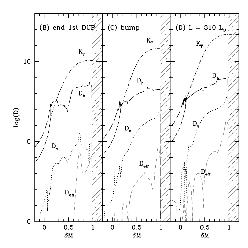
Figure 5: Same as Fig. 4 for M2 in Table 1. M2 only differs from M1 by the adopted differential rotation law in the convective envelope

The profile of $D_{\rm eff}$ in Fig 5 appears to be quite ragged below $\delta M\simeq 0.5$, in particular on panel (D). Each of the bump in this region is associated with an inversion of the meridional circulation velocity, which can be positive or negative. Although the meridional circulation can actually present various cells, these particular features are due to numerical instabilities occurring in the regions where the mean molecular weight gradients are non-negligible. When the effects of $\mu$-currents are included (terms depending on $\mu$ or $\Lambda$ in Eq. 2), the numerical system is highly non-linear and may be sensitive to numerical parameters such as the spatial and temporal resolutions.
The global amplitude of $D_{\rm eff}$ (and $D_{v}$) in these regions of large $mu$-gradients, together with the decrease in the diffusion coefficients in the nuclearly active shells are however robust results. Just below the CE, the first bump in the $D_{\rm eff}$ profile is also a robust feature, associated with the Gratton-Öpik meridional circulation cell. These remarks apply to all our models.

5.2 Impact of the ZAMS rotation velocity

We investigated the impact of the initial rotational velocity considering an originally slow (model M2) and a fast rotator (model M6) on the ZAMS, without changing any of the other physical parameters. We have applied to model M6 the same treatment as to Pop I stars (see paper I), namely a strong magnetic braking according to the Kawaler (Kawaler88 (1988)) prescription so as to get a surface equatorial velocity lower than 10 $\>{\rm km}.{\rm s}^{-1}$ before the central hydrogen mass fractions gets lower than 0.5. At the turn-off the surface velocities of models M6 and M2 are thus quite similar (see Table 3).
The point under scrutiny in this section is to determine whether this strong braking, which triggers strong turbulence in the radiative zone during the main sequence, has an incidence on the angular momentum distribution and on the diffusion coefficients beyond the turn-off.
In the present study, we did not investigate the case of fast rotators at the turn-off, this configuration being ruled out by the velocities available from observations of low-mass turn-off stars in globular clusters (Lucatello & Gratton LG03 (2003)).

Figure 2 presents the degree of differential rotation ($\theta$ profiles) and the angular velocity inside models M2 and M6 (dotted and dashed lines respectively) at different evolutionary points. Model M6 rotates globally faster than model M2 at the turn-off, and this difference is maintained during the evolution. Indeed, although model M6 undergoes a very efficient braking on the early MS, it is only braked down to 5.7 $\>{\rm km}.{\rm s}^{-1}$ at the turn-off, compared to 3.88 $\>{\rm km}.{\rm s}^{-1}$ in model M2. In spite of these different surface rotation rates, the profiles of $\Omega$ and $\theta$ are quite similar in the radiative zone of these models during the RGB phase (Fig. 3). Consequently, the turbulent diffusion coefficients (see Eq. 7) are not very different during the RGB phase, as can be seen on Figs. 5, 6 and  10.

This comparison shows that the structural readjustments (induced the 1st DUP) efficiently redistribute the AM throughout the star beyond the turn-off. The resulting rotation profile after the completion of the 1st DUP is almost solely determined by the star’s total angular momentum at the turn-off and by the CE rotation law.

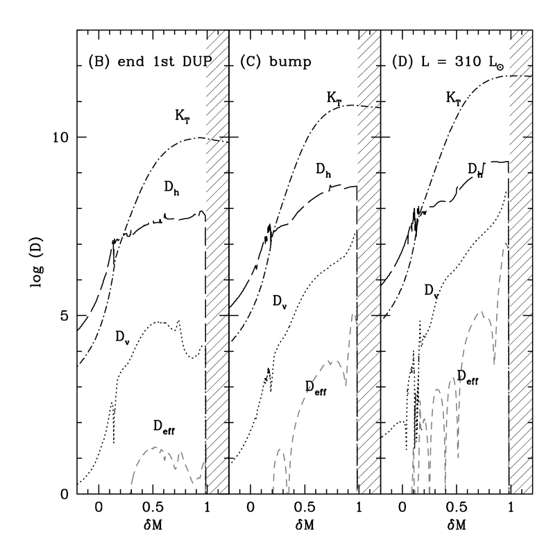
Figure 6: Same as Fig. 4 for M6. In this model, $\upsilon_{\rm ZAMS}=110\leavevmode\nobreak\ {\rm km}.{\rm s}^{-1}$ and after efficient braking through according to a Kawaler law , $\upsilon_{\rm TO}=6.4\leavevmode\nobreak\ {\rm km}.{\rm s}^{-1}$

. Uniform specific angular momentum was assumed in the CE.

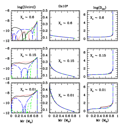
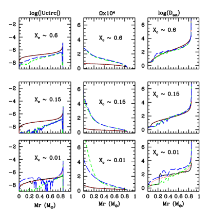
Figure 7: Profiles of the vertical component of the meridional circulation velocity $U_{r}$, angular velocity $\Omega$ and total diffusion coefficient $D_{\rm tot}$ inside $0.85\,$${\rm M_{\odot}}$, [Fe/H] = -1.57 models at three stages of their evolution (as indicated by their central H content $X_{c}$ : $X_{c}=0.6\Leftrightarrow t\approx 2\leavevmode\nobreak\ Gyr$, $X_{c}=0.15\Leftrightarrow t\approx 8\leavevmode\nobreak\ Gyr$ and $X_{c}=0.01\Leftrightarrow t\approx 10\leavevmode\nobreak\ Gyr$). First 3 columns on the left Profiles for models that are slow rotators on the ZAMS ($\upsilon_{ZAMS}=5\>{\rm km}.{\rm s}^{-1}$) and undergo no braking.Last 3 columns on the right Profiles of initially fast rotating models on the ZAMS ($\upsilon_{ZAMS}=110\>{\rm km}.{\rm s}^{-1}$) and undergoing strong magnetic braking during their early MS evolution. Here, solid and dashed lines are superimposed and indistinguishable from one another. Details on input parameters are given in Table 2.

5.3 $\mu$-currents and horizontal turbulence

The mean molecular weight affects the transport of chemicals via its gradient $\nabla_{\mu}$ and its relative horizontal variation $\Lambda$ (see Eqs. 2 and A). $\mu$-gradients inhibit the efficiency of meridional circulation, and $\mu$-currents are inhibited by strong horizontal turbulence. In paper I we emphasised the importance of these terms in establishing the differential rotation profile during the MS for Pop I stars.

In order to better assess the role of $\mu$-currents in Pop II stars, and to determine their sensitivity to the horizontal turbulence description, we have computed a series of models for which we alternately use the $Zahn92$ and the $MPZ04$ prescriptions for $D_{h}$, assuming both $E_{\mu}=0$ and $E_{\mu}\neq 0$, and $\upsilon_{ZAMS}=5\>{\rm km}.{\rm s}^{-1}$ and $\upsilon_{ZAMS}=110\>{\rm km}.{\rm s}^{-1}$ for each case. The properties of these models are summarised in Table 2.

Main sequence

Let us first comment on the MS evolution. The profiles of $\Omega$, $U_{r}$ and $D_{\rm tot}$ are displayed on Figure 7 at three different times on the MS (see Table 2 for detailed description of each curve).

Table 2: Input parameters for the models discussed in §5.3. Some of the models appearing in this table are also listed in Tab. 1. Models Ma, Mb, Mc, Md and Mh have only been computed up to the turn-off. In all models, solid-body rotation in the CE has been assumed, and $D_{v}$ is given by TZ97.

Model	$\upsilon_{\rm ZAMS}$	Braking	$D_{h}$	$\mu$-currents	line style
	$\>{\rm km}.{\rm s}^{-1}$				in Fig. 7
Ma	110	yes	MPZ04	no	solid
Mb	110	yes	MPZ04	yes	dotted
Mc	110	yes	Zahn92	yes	short-dashed
Md	110	yes	Zahn92	no	long-dashed
M3	5	no	MPZ04	no	solid
M2	5	no	MPZ04	yes	dotted
M5	5	no	Zahn92	yes	short-dashed
Mh	5	no	Zahn92	yes	long-dashed

Slow rotators on the ZAMS (Fig. 7, left panels).

Their slow rotation together with the negligible structural readjustments occurring during the MS does not favour any mechanism able to trigger steep rotation profiles. As a result, the transport of both angular momentum and chemicals by rotation-induced processes is inefficient. This is independent of the choice for the $D_{h}$ prescription and of the introduction or not of the $\mu$-currents. The $\Omega$-profile as well as the total diffusion coefficient for chemicals is similar in all cases. $\mu$-gradients in the radiative interior are small, which makes the effects of $\mu$-currents negligible during the MS.

Fast rotators on the ZAMS (Fig. 7, right panels).

Turning now to the fast rotators on the ZAMS, the strong braking at the beginning of the MS allows the build-up of steeper $\Omega$-gradients, and shear-turbulence can develop across the radiative zone already during the main sequence. This leads to efficient transport of both angular momentum and chemicals, similarly to what is obtained in their Pop I counterparts. The $\mu$-gradients are larger in this case than for slow rotators, and we can expect $\mu$-currents to have the same effects on the rotation profile as those observed in the Pop I stars. It is actually the case when considering the Zahn92 prescription for $D_{h}$ which was used in paper I. As shown on Fig 7, when the $\mu$-currents are taken into account ($E_{\mu}\neq 0$; short-dashed lines), the degree of differential rotation reached near the end of the MS is substantially larger than when these terms are neglected (long-dashed lines). The $\mu$-currents also limit the extent of the shear unstable region at the centre, whereas when $E_{\mu}=0$, turbulence is free to develop across the entire radiative interior (third column, Fig. 7).

Using the MPZ04 for $D_{h}$ leads to a different conclusion. This prescription produces much larger values for the horizontal turbulence $D_{h}$ than the former one. As the $\mu$-currents ($E_{\mu}$ term in Eq. 2; see also Eq. A in Appendix) are generated by the horizontal variation of the mean molecular weight, they are much reduced by this choice. In the case we are considering, they are reduced to an insignificant level, i.e. they remain small compared to the $\Omega$-currents (term $E_{\Omega}$ in Eq. 2; see also Eq. LABEL:eom) and do not affect the rotation profile nor the meridional circulation velocity.

In short, on the MS, the $\mu$-currents have negligible effects on Pop II low-mass stars that are slow rotators, independently of the prescription used for $D_{h}$. This is exclusively due to the slow rotation. On the other hand, the $\mu$-currents may affect the building of the rotation profile during the MS evolution of low-mass Pop II stars undergoing strong magnetic braking if the horizontal turbulence is not too large to prevent any significant variation of the mean molecular weight to develop.

Red Giant Branch

Comparing model M2 with model M3 and M5 provides respective clues on the effects of the $\mu$-currents (M2 versus M3) and the horizontal turbulence description (M2 versus M5) on the transport of chemicals beyond the turn-off.
Figure 10 presents the total diffusion coefficients for the chemicals in all our rotating models at evolutionary points (B), (C) and (D). $D_{\rm tot}$ in models M2, M3 and M5 (dotted, long-dashed dotted and long-dashed lines respectively) is essentially the same at the different evolutionary points presented. This indicates that $\mu$-currents do not affect the transport of chemicals on the RGB. On the other hand, the choice of the prescription for horizontal turbulence has small effects on $D_{\rm tot}$. This is due to the fact that $D_{h}$ essentially affects the effective coefficient $D_{\rm eff}$, which is much smaller than $D_{v}$ after the 1st DUP in case Zahn92 is used, and remains small for MPZ04. Let us add that in general, $D_{h,MPZ04}>D_{h,Zahn92}$, and that for $D_{h,Zahn92}$, the shellular rotation hypothesis (i.e. $D_{h}\gg D_{v}$) is violated in some regions (see panel (D) Fig. 8).

5.4 Vertical turbulent diffusion coefficient

In order to compare our results with the calculations of Denissenkov & Tout (DT00 (2000)), we also computed a model (M4) using the MM96 prescription for $\nu_{v}$ (Eq. 6). The main differences between this criterion and the one derived by Talon & Zahn (TZ97 (1997)) were already exposed in § 3.4. In Fig. 9 we present the diffusion coefficients for model M4 at the end of the 1st DUP at the bump and at L $\simeq 310\leavevmode\nobreak\ \>{\rm L_{\odot}}$. Contrary to models M2, M3, M5 and M6, for which we also assumed uniform specific angular momentum in the CE beyond the turn-off, by the end of the 1st DUP, the shear instability has not developed between the base of the CE and the edge of the HBS in model M4. Indeed Eq. (6) shows that the shear must be larger than $N^{2}_{\mu}$ for the instability to develop. In the case of giants, it is only after completion of the 1st DUP, where the retreating CE leaves a chemically homogeneous region ($N^{2}_{\mu}=0$), that the shear instability may set in. However the CE remains disconnected from the nucleosynthesis regions until the large $\mu$-barrier left by the DUP is erased at the bump. This justifies the assumption of Denissenkov & Tout (DT00 (2000)), that considers rotational transport of chemicals only from the bump on.

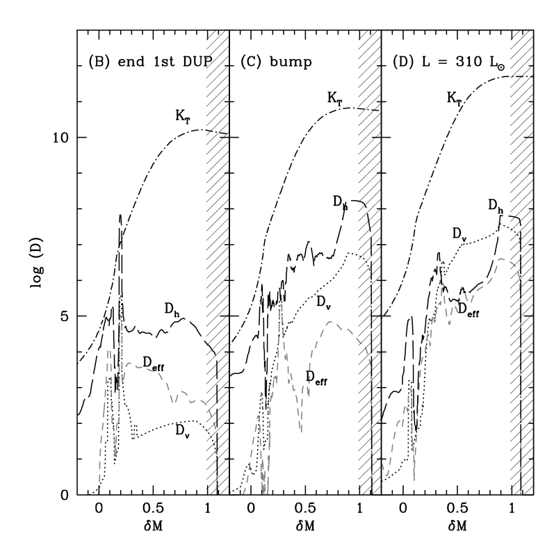
Figure 8: Same as Fig. 4 for M5. This model is similar to M2 but was computed using the Zahn (1992) expression for $D_{h}$.

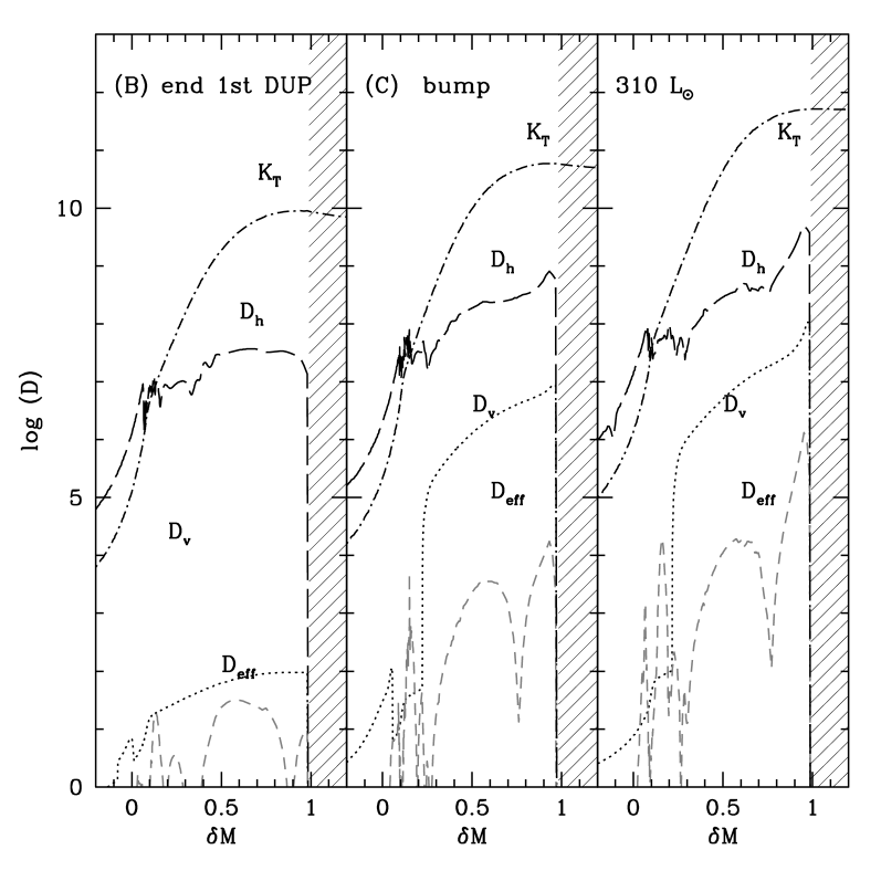
Figure 9: Same as Fig. 4 for M4. This model is similar to M2 except that the prescription for the vertical turbulent diffusion coefficient is that of Maeder & Meynet (1996).

Figure 10: Lower panels Total diffusion coefficient for several models (line encoding is given in the figure) as a function of the reduced mass coordinate $\delta M$ at the end of the first dredge-up and at the bump.Upper panels Hydrogen mass fraction profiles in the same models.

However, Meynet & Maeder (MM97 (1997)) showed that using this strong criterion prevents mixing from occuring in massive, fast rotating stars, in contradiction with observational evidence. The same conclusion that was also reached by Talon et al. (TZMM97 (1997)), and motivated the authors to introduce the erosion of the $\mu$-gradient by horizontal turbulence. For the same reason, Maeder (M97 (1997)) also developed a modified shear criterion to reduce the efficiency of mean molecular weight gradients.

Being in the same framework (i.e. study of transport associated with meridional circulation and shear turbulence), and in absence of strong observational evidence, it is not justified to change these prescriptions for the particular case of low-mass RGB stars. It was SM79 who first suggested that prior to the bump, mixing should be hindered by the $\mu$-barrier left at the end of the 1st DUP, and that surface abundance variations should not be expected before this evolutionary point. We will show however in the following that a mixing process eroding the $\mu$-gradient does not necessarily alter the surface abundance pattern prior to the bump.

5.5 Dominant process for the transport of angular momentum and chemicals

In the framework of this paper, we consider two transport processes, namely meridional circulation and turbulence induced by the secular shear instability. Whereas shear-induced turbulence is always described as a diffusive process, meridional circulation appears as an advective process for AM and as a diffusive process for the chemical species (Eq. 1 and Eq. 5 respectively). The relative importance of these processes can thus be different depending on whether we consider AM or elements transport.
In the case of chemical species, Figs. 4–6 and 8–9 indicate clearly that shear-induced turbulence is the dominant transport process beyond the completion of the 1st DUP when uniform specific angular momentum is assumed in the envelope. The exception is model M5, where due to the smaller efficiency of the horizontal shear turbulence ($D_{h}$ = $D_{h,Zahn92}$), meridional circulation is large and still dominates the transport of chemicals at the end of the 1st DUP (Fig. 8). Higher on the RGB however, turbulence recovers the upper hand in this model too. For model M1, shear-induced turbulence can not be triggered in the radiative zone after the 1st DUP, and meridional circulation accounts for transport for chemicals. The value of $D_{\rm eff}$ remains however always smaller that the molecular viscosity $\nu_{mol}$.

In order to estimate the efficiency of the two processes responsible for the AM transport, we compare their relative characteristic timescales. The characteristic timescales for AM transport by meridional circulation and by shear-induced turbulence over a distance $\Delta r$ can be estimated as $\tau_{U}\sim\frac{\Delta r}{U_{r}}$ and $\tau_{\nu}\sim\frac{(\Delta r)^{2}\Omega}{D_{v}\Delta\Omega}$ respectively.
$\tau_{U}<<\tau_{\nu}$ at the end of the 1st DUP for all models but model M1. This situation is subsequently modified as shells with a large angular momentum are incorporated from the inner CE into the radiative interior. From the bump on, the efficiency of turbulence becomes thus similar to that of meridional circulation, with $\tau_{\nu}\simeq\tau_{U}\sim 10^{5}$ yr. For model M1, $\tau_{\nu}\simeq\tau_{U}\simeq 10^{7}$ yr from $\delta M\sim$ 0.1 to 0.8 at all times (evolutionary points (B), (C) and (D)). In the region just below the CE, for $\delta M\in[0.8;1]$, the degree of differential rotation is very small (see Fig. 2) so that the timescale for AM transport by turbulence is of the order of 10 Gyr, and meridional circulation dominates.

Between the turn-off and the completion of the 1st DUP, meridional circulation dominates the transport of AM in all our models, while the chemical species are mainly transported through turbulence. Beyond the 1st DUP, chemicals are transported via shear-induced turbulence while the AM essentially evolves due to structural readjustments. Indeed at this phase, the advective (meridional circulation) and the diffusive (shear-induced turbulence) processes almost compensate each other, letting the Lagrangian term control the evolution of the angular velocity profile. In those models where turbulence can not develop, meridional circulation dominates the transport of chemicals and AM (model M1).
The dominant transport process for AM can thus differ from the process controlling the transport of chemicals. It can also vary along the evolution.

6 Signatures of mixing

6.1 Structure evolution

Through the transport of chemicals, and in particular those contributing to the nuclear energy production and the opacity, rotation may indirectly affect the evolution of stars in terms of lifetimes, luminosities and effective temperatures. Centrifugal forces can also affect the structure but this effect is negligible for the low rotation rates considered here.

6.1.1 Main Sequence

Figure 1 presents the Hertzsprung-Russell (HR) diagram for the models listed in Table 1. Models M0 to M3 can hardly be distinguished on the figure. Due to their small initial rotation velocity and the absence of braking to pump AM, models M1 to M3 present very weak differential rotation resulting in inefficient mixing during the MS phase ($D_{\rm tot}\approx 10^{2}-10^{3}\leavevmode\nobreak\ {\rm cm}^{2}{\rm s}^{-1}$); their evolution as well as their chemical structure is thus only scarcely affected by rotation-induced mixing. Table 3 presents the main evolutionary characteristics of our models. The luminosity and effective temperature at the turn-off, as well as the time spent on the MS are similar in slowly rotating (M1-M5) and standard (M0) models.

Model M6 deviates from the standard and slow-rotating tracks. In this model, the strong braking applied during the first million years spent on the MS creates a large differential rotation inside the star leading to an efficient transport of the chemicals (see Eq. 7). In this case, as helium diffuses outwards, the opacity is globally lower and the star consequently bluer and more luminous. As a result of fuel replenishment due to efficient rotational mixing, the H burning phase also lasts for $\approx 400$ Myr longer in model M6, which is thus older at the turn-off compared to the other rotating models (Table 3).

For all our rotating models, the surface velocity at the end of the MS is lower than 6 $\>{\rm km}.{\rm s}^{-1}$, in fair agreement with the upper limits derived for globular clusters MS stars (Lucatello & Gratton LG03 (2003)). During the MS evolution, the surface rotation velocity remains almost constant in models M1 to M5. They are slowed from 5 $\>{\rm km}.{\rm s}^{-1}$ on the ZAMS to $\approx 4\leavevmode\nobreak\ \>{\rm km}.{\rm s}^{-1}$ at the turn-off mainly due to the structural readjustment that become important at the end of this phase. Model M6 undergoes magnetic braking on the MS so that its rotational velocity has already dropped below $\approx 6\leavevmode\nobreak\ \>{\rm km}.{\rm s}^{-1}$ when the model reaches the middle of the main sequence (i.e. for $X_{c}\simeq 0.5$). This velocity further decreases due to the efficient transport of AM in the radiative interior, and reaches 5.7$\>{\rm km}.{\rm s}^{-1}$ at the turn-off.

Table 3: Main evolutionary features of the models presented in Table 1. TO index stands for turn-off values. $M_{\rm BCE,DUP}$ is the mass coordinate associated with the deepest extension of the convective envelope during the first dredge-up. $\Delta t_{\rm bump}$ is the time needed for the entire HBS to pass through the $\mu$-discontinuity left by the 1st DUP.

Model	0	1	2	3	4	5	6
$t_{\rm TO}$ (Gyr)	11.11	11.20	11.21	11.21	11.21	11.21	11.61
$L_{\rm TO}$ ($\>{\rm L_{\odot}}$)	3.35	3.34	3.35	3.35	3.35	3.35	3.55
$T_{\rm eff,TO}$ (K)	6534	6547	6543	6543	6543	6543	6582
$\upsilon_{\rm TO}$ ($\>{\rm km}.{\rm s}^{-1}$)	0	3.88	3.90	3.89	3.85	3.95	5.71
$M_{\rm BCE,DUP}$ ($\>{\rm M_{\odot}}$)	0.306	0.303	0.304	0.306	0.304	0.307	0.306
$L_{\rm bump}$ ($\>{\rm L_{\odot}}$)	107	101	109	113	103	110	114
$T_{\rm bump}$ (K)	4899	4919	4897	4887	4910	4896	4897
$\Delta t_{\rm bump}$ (Myr)	4.87	7.14	7.75	6.28	5.75	6.68	7.73

6.1.2 Red Giant Branch

The large increase in radius accompanying the deepening of the convective envelope during the 1st DUP, combined with global conservation of AM, leads to very efficient braking of the surface layers and spin-up of the core. All our rotating models have surface velocities lower than 1$\>{\rm km}.{\rm s}^{-1}$ at the end of the dredge-up (including model M6 for which we have $\upsilon_{ZAMS}=110\>{\rm km}.{\rm s}^{-1}$). In models M1, M2, M4 and M6, for which the total diffusion coefficient for chemicals is larger than the molecular viscosity at the base of the envelope, the 1st DUP is deeper compared to the standard case. These variations of the depth of the 1st DUP (Tab. 3) remain however small and will not affect significantly the surface abundance patterns at this phase (see § 6.2, Fig. 15).

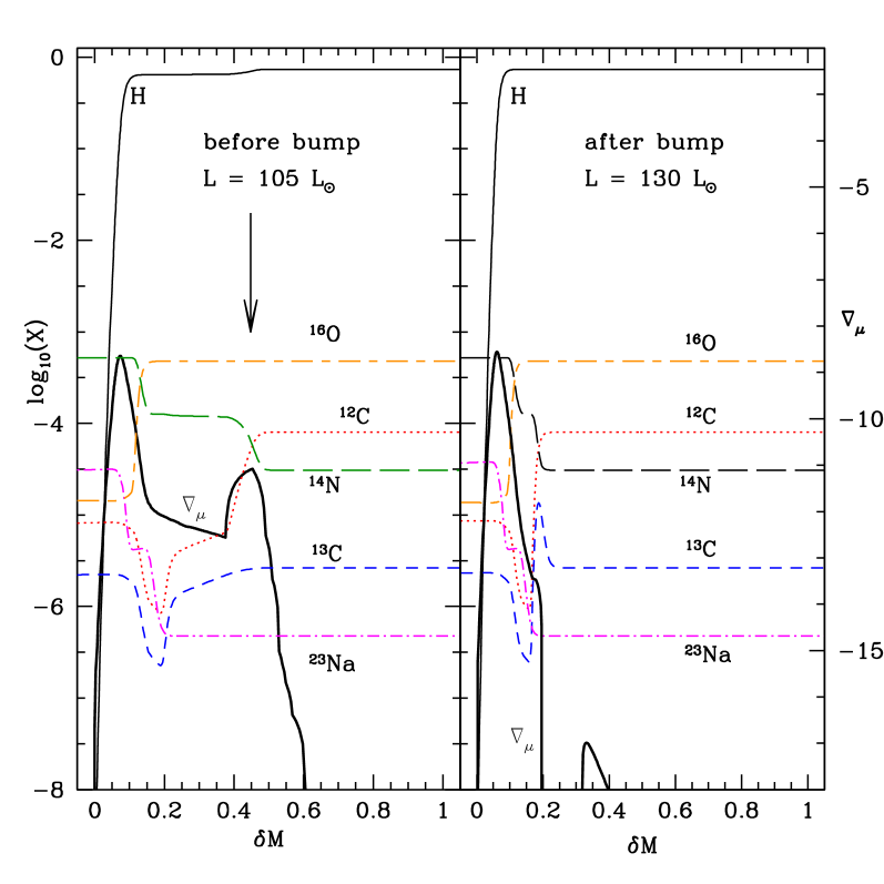
Figure 11: Logarithm of the mass fraction profiles of H, ${}^{12}{\rm C}$, ${}^{13}{\rm C}$, ${}^{14}{\rm N}$, ${}^{16}{\rm O}$, ${}^{23}{\rm Na}$ and of the mean molecular weight gradient $\nabla_{\mu}=d\ln\mu/dr$ (bold line) as a function of the reduced mass inside a $0.85\,$${\rm M_{\odot}}$, $Z=0.0005$ standard stellar model M0. The panels represent the profiles of these elements in the HBS just before (i.e. before the HBS contacts the $\mu$-discontinuity left by the 1st DUP) and after (i.e. once the mass coordinate at the base of the HBS is larger than $M_{\rm BCE,DUP}$) the bump. In the left panel, the down-going arrow indicates the mass coordinate of maximum penetration of the CE during the 1st DUP.

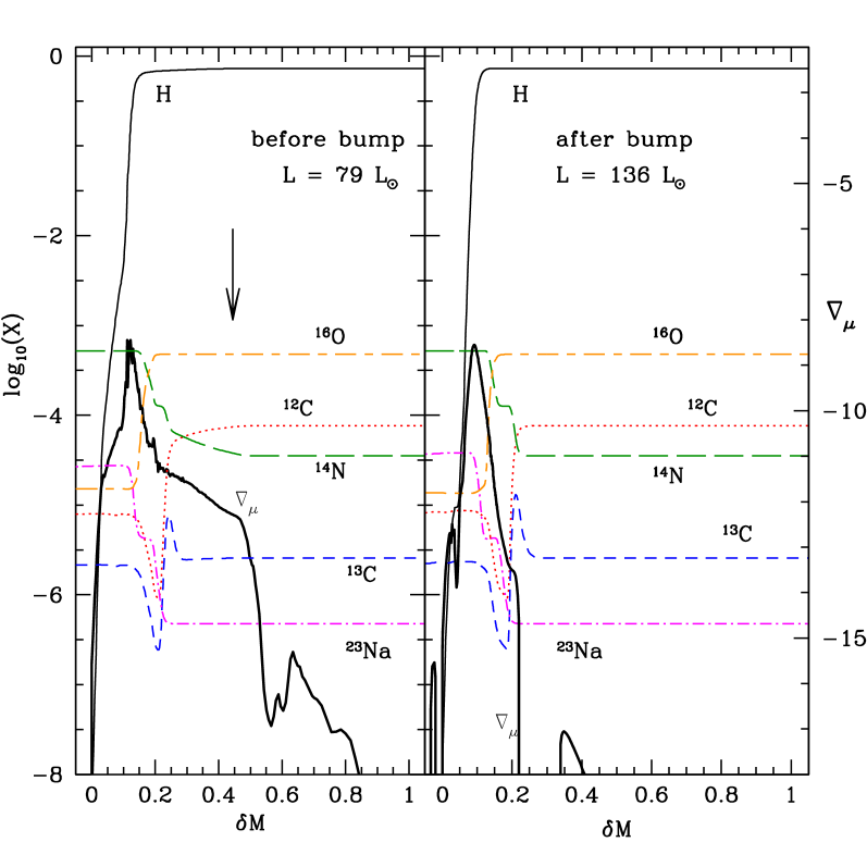
Figure 12: Same as Fig. 11 for our rotating reference model M1.

In the following we will refer to the bump luminosity as the luminosity of the model when the mass coordinate of the maximum energy production inside the HBS is equal to ${\rm M}_{\rm BCE,DUP}$.

Figures 11, 12 and 13 present selected abundance profiles and the mean molecular weight gradient $\nabla_{\mu}=\partial\ln\mu/\partial r$, before and after the bump inside models M0, M1 and M6 respectively. The peak amplitude $\nabla_{\mu,c}$ in the $\mu$-gradient profile at $M_{r}=M_{\rm BCE,DUP}$ (indicated by an arrow on the left panels) decreases with increasing degree of mixing. In the non-rotating model, this peak is a signature of the deepest penetration of the convective envelope during the first dredge-up, and the corresponding $\nabla_{\mu,c}$ value is $\simeq 10^{-11}$ (Fig. 11). In the rotating models, the peak is spread out due to the ongoing transport of the chemicals and varies between $\nabla_{\mu,c}\simeq 3\cdot 10^{-12}$ (Fig. 12) and $\nabla_{\mu,c}\simeq 5\cdot 10^{-13}$ (Fig. 13). The amplitude of $\nabla_{\mu,c}$ directly reflects the strength of the diffusion coefficient in this area (see Figs. 4 and 6). According to Charbonnel et al. (CBW98 (1998)) the regions where $\nabla_{\mu}\geq 1.5\times 10^{-13}$ should not be affected by the extra-mixing acting below the CE. Therefore, even the low value of $\nabla_{\mu,c}$ found in model M6 can prevent mixing to act freely below $\delta M\approx 0.5$.
Let us finally emphasise that although the amplitude of the diffusion coefficients may be locally increased due to numerical instabilities, and artificially lower the mean molecular gradient in that region, the reproducibility and constancy of the $\mu$-barrier spread over indicates that this feature is not a numerical artifact.

In order to evaluate the “observational” impact of rotational mixing on the luminosity function’s bump, we have computed theoretical luminosity functions (hereafter LF) for each of our models (see Fig. 14). These theoretical LF represent the time spent in each bin of magnitude V by models on the RGB with magnitudes lower than $V=16.6$. We have chosen this cut-off in order to be able to compare the models predictions with the observed luminosity function of the globular cluster M13 as given by Cho et al. (2005).

In order to determine the $V$ magnitude associated with a given luminosity $L$, we used the classical magnitude-luminosity relation

$$V=M_{bol,\odot}-2.5\log(L/L_{\odot})-{\rm BC}+(m-M)_{V}.$$

For M13, we adopt a distance modulus $(m-M)_{V}=14.48$ , following Cho et al. (2005), and a bolometric correction ${\rm BC}=-0.253$, according to the value given by Girardi et al. (2002) for [Fe/H] $=-1.5$, $T_{\rm eff}=5000\leavevmode\nobreak\ {\rm K}$ and $\log g=2$. $M_{bol,\odot}=4.76$ according to Cox (Cox2000 (2000)).

Figure 14 emphasises the following points :

1. The bump clearly appears for all models in spite of the numerical noise present at higher magnitudes in models M2 and M6. When the $\mu-$barrier has been efficiently eroded, the bump is less pronounced in the LF.

2. The predicted LF for models with low degree of mixing (namely M1, our reference model, and M3, with $E_{\mu}=0$) are similar to the one obtained for the standard model M0. In case of model M3, the diffusion coefficient in the outer HBS remains always small prior to the bump (i.e. $D_{\rm tot}\leq 5.10^{3}\leavevmode\nobreak\ {\rm cm^{2}.s^{-1}}$). This allows preservation of a large $\mu$-gradient which is responsible for the clear signature in the LF. A similar effect explains the LF for model M1, where transport efficiency is always low in the radiative zone.

3. In rotating models, the bump occur at higher luminosity compared to the standard model M0.

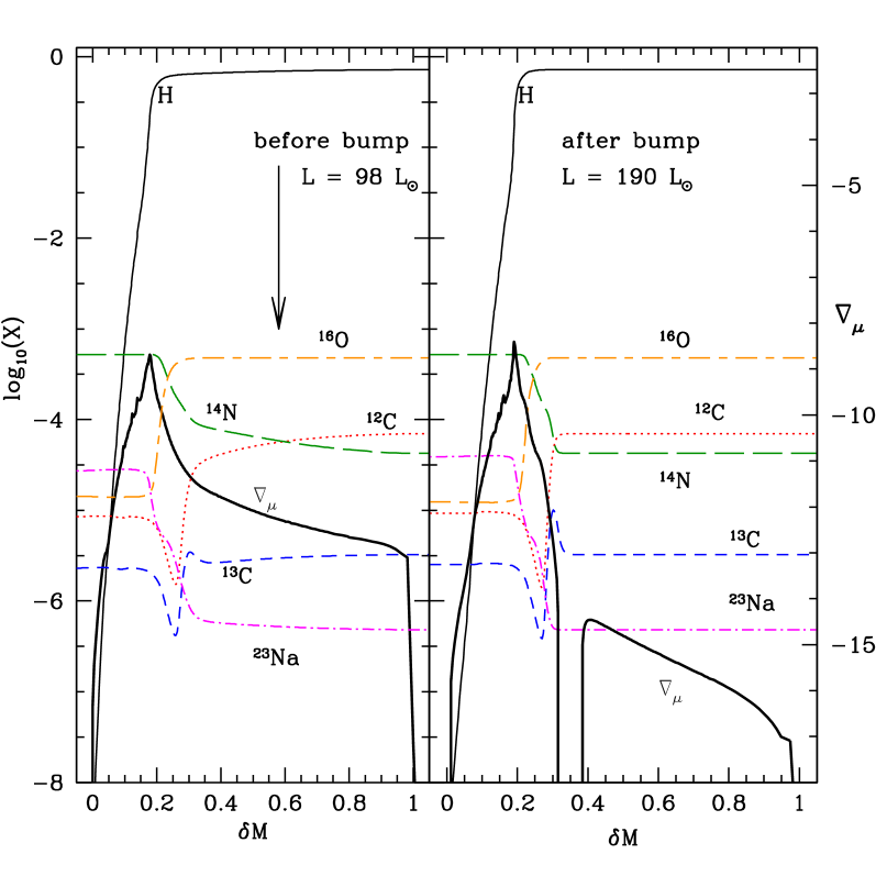
Figure 13: Same as Fig. 11 for model M6.

6.2 Abundances

In § 6.1, we mentioned the lowering of the mean molecular weight barrier left by the 1st DUP in rotating models M1 and M6. Figure 12 shows the erosion of ${}^{12}{\rm C}$ and ${}^{14}{\rm N}$ profiles as a result of rotational mixing. However, this chemical diffusion does not affect significantly the surface abundances, and we report only a minor increase of ${}^{14}{\rm N}$ anti-correlated with a decrease of ${}^{12}{\rm C}$ compared to the standard case.

In Model M6 the higher degree of differential rotation at the base of the CE feeds the turbulent shear-induced mixing. The outer ${}^{14}{\rm N}$ plateau is erased and the nitrogen mass fraction in the CE is increased relative to the standard case. ${}^{13}{\rm C}$ also diffuses outwards and the peak around $\delta M=0.3$ is flattened out. Although the mean molecular weight at the depth of deepest penetration of the CE is much lower than in the standard model, $D_{v}$ (which dominates the transport) decreases rapidly from $10^{9}\,{\rm cm}^{2}{\rm s}^{-1}$ just below the CE down to $\approx 10^{5}\,{\rm cm}^{2}{\rm s}^{-1}$ in the chemically inhomogeneous regions of the outer HBS (Fig. 8). Mixing is thus confined to a narrow region located just below the CE, where the chemical profiles are flat. According to Charbonnel (1995) and Denissenkov & VandenBerg (DV03 (2003)), diffusion coefficients as large as $\approx 4\cdot 10^{8}\,{\rm cm}^{2}{\rm s}^{-1}$ are needed to connect the HBS with the CE and to modify the surface abundances. However this configuration is never reached in our self-consistent models.

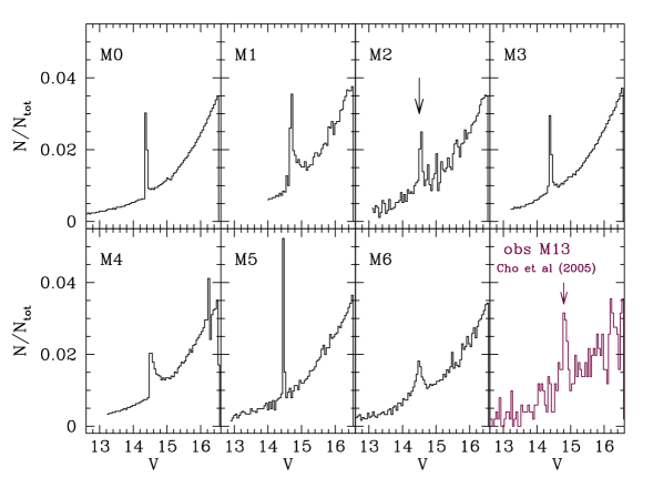
Figure 14: Normalised theoretical luminosity function in V for the models presented in Table 1 and 3. These histograms represent the time spent in each magnitude (luminosity) bin as a function of visual magnitude V. The ordinates are normalised to the total time spent on the portion of the RGB where V $\leq 16.6$. This limit has been chosen in order to have the same normalisation as in the observational case presented in the $8^{th}$ panel (low right). The observed normalised luminosity function is based on Cho et al. (2005). The arrows in panels 3 and 8 indicate the position of the bump.

We reach similar conclusions for the other rotating models, since at the bump, the diffusion coefficients have the same magnitude, and are too small to affect the surface abundance composition. This is clearly illustrated in Fig. 15, where we present a comparison of the temporal evolution of lithium, carbon, nitrogen and carbon isotopic ratios obtained in our models with homogeneous observational data for field stars with [Fe/H] $\in[-2;-1]$. While variations associated with the 1st DUP are satisfactory and rotating models tend to better agree with observations, no further variations are obtained after the bump. Let us note that model M6 leads to the destruction of lithium already on the MS (because of strong mixing associated with the shear in absence of any compensating mechanism) in contradiction with the observations. This situation is similar to that encountered in Pop I stars on the red side of the lithium dip. For a complete discussion of this problem, the reader is referred to Talon & Charbonnel (TC98 (1998)), as well as to Talon & Charbonnel (TC05 (2005)) and Charbonnel & Talon (CT05 (2005)) which describe how internal gravity waves could help resolve this issue in Pop II stars.

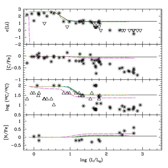
Figure 15: Evolution of the lithium abundance ($\epsilon(^{\rm 7Li})$), the carbon isotopic ratio ${}^{12}{\rm C}/^{13}{\rm C}$, [C/Fe] and [N/Fe] as a function of the luminosity logarithm for the models presented in Table 1. Line encoding is the same as in Fig. 1. Black asterisks are actual measurements, open upward triangles are lower limits and open downward triangles are upper limits. Observational data from Gratton et al. (2000) for field stars in the metallicity range $[{\rm Fe/H}]\in[-2;-1]$.

Regarding lithium on the RGB the mixing rates associated with shear-induced turbulence do not allow the triggering of the Li-flash as proposed by Palacios et al. (PCF01 (2001)) to consistently explain the low percentage of lithium rich giants at the bump luminosity. Indeed, in this scenario, an initial mixing rate of about $10^{9}{\rm cm}^{2}.{\rm s}^{-1}$ is needed in the region of the ${}^{7}{\rm Be}$ peak region in order for it to diffuse outwards and decay into ${}^{7}{\rm Li}$ in a region where this nuclide will efficiently capture protons and give rise to a energetic runaway called the “Li-flash”. We never get such high mixing rates in the radiative interior of our models.
The present description of the extra-mixing process in RGB stars does not allow the models to reproduce the observed abundance anomalies in upper RGB stars, and does not validate the Li-flash scenario for Li-rich RGB.

7 Comparison with previous works

In this paper we have presented the first models of rotating low-mass stars which take into account rotational transport by meridional circulation and shear turbulence coupled self-consistently to the structural evolution from the ZAMS to the upper RGB. A detailed study of the input physics associated with the rotational transport of angular momentum and chemicals allowed us to assess the impact of various physical ingredients on the extension and magnitude of mixing along the giant branch. Let us know compare our predictions with others from the literature

1. Angular momentum evolution
   

   With regard to the evolution of the angular velocity profile, we assumed solid body rotation on the ZAMS in all our models and then let angular momentum be transported by meridional circulation and shear-induced turbulence. At the turn-off, this leads, in all cases, to differential rotation in the radiative interior and to a slowly rotating convective envelope. Beyond the turn-off, the angular velocity below the CE is determined by the assumed rotation law in the CE. Both the absolute value of $\Omega_{\rm BCE}$ and the degree of differential rotation (and hence mixing) in the radiative zone are maximised after the completion of the 1st DUP in the case of a differentially rotating CE ($j_{\rm CE}(r)=cst$). This supports the conclusions anticipated by other authors. In 1979, Sweigart & Mengel conjectured that differential rotation in the convective envelope of a red giant with homogeneous specific angular momentum could be necessary to provide enough rotational mixing at the bump. Recently, Chanamé et al. (CPT05 (2005)), using a “maximum mixing approach”, reach the same conclusion from considerations on the global AM budget. They also indicate that if $\Omega$ has to be described by a power law, it is not necessarily with a -2 index (e.g. uniform specific angular momentum). As we mentioned in § 3.5, assuming uniform specific angular momentum is a first approximation, and we may expect better estimates of the CE rotation regime from direct numerical simulations.
   In their work, Chanamé et al. (CPT05 (2005)) nonetheless insist on the fact that in order for rotational mixing to reproduce the observed abundance anomalies of low-mass Pop II RGB stars, they need to assume unrealistic large rotation velocities at the turn-off. This is a conclusion that we also reach in our complete computations. Differential rotation in the radiative region separating the HBS from the CE increases as the CE retreats after the DUP. However, all together, the self-consistent evolution of the rotation profile for realistic surface velocities at all phases leads to transport coefficients too low by 3 orders of magnitude compared to what is expected from parametric studies (Weiss et al. WDC00 (2000), Denissenkov & VandenBerg DV03 (2003)) in order to alter the surface chemical composition beyond the bump luminosity and reproduce the observed patterns.

   In this work, we did not force the specific angular momentum to have the same value at all times in the convective envelope , as was done by Denissenkov & Vandenberg (DV03 (2003)). Under such an assumption the specific angular momentum within the CE remains at the same level during the 1st DUP as at the turn-off, which results in an increase of the differential rotation and mixing below the CE. On the contrary, in the models M2 to M6 presented here, when the CE deepens during the 1st DUP, it dredges material with lower specific angular momentum, and $j_{CE}$ (which is the same in each mass shell within the CE) drops as can be seen from Fig. 3. As a result, the angular velocity and the differential rotation are lower at the bump. Beyond the completion of the 1st DUP, $j_{CE}$ continues to evolve slightly due to angular momentum transfer with the underlying radiative zone, but does not significantly vary anymore. Assuming no variation in space of the specific angular momentum in the CE after the turn-off appears to be very different from assuming no variation with time of this same quantity. This latter assumption, when combined to strong differential rotation in the radiative interior on the MS, is an ad hoc way to produce strong differential rotation (and mixing) at the bump.

   Although Denissenkov and collaborators (Denissenkov & Tout DT00 (2000) ($DT00$), Denissenkov & VandenBerg DV03 (2003) ($DV03$)) have also searched for a solution to the RGB abundance anomalies problem in terms of rotational mixing by meridional circulation and shear turbulence, they reach very different conclusions in terms of the evolution of the surface abundance pattern on the RGB. As a matter of fact, their transport coefficients are very similar to ours in terms of shape, but they get at all phases much larger rotation velocities and differential rotation rates than we do, resulting in higher mixing rates.

   The origin of the differences is difficult to assess although several points are certainly critical. First of all the self-consistency of the treatment of rotational transport within the stellar evolution code, which allows the retro-action of AM and chemicals transport on the structure at each evolutionary step seems to be crucial. Although $DT00$ solved Eq. 1 using Maeder & Zahn (MZ98 (1998)) formalism, this was done outside their evolution code in a post-processing way. In addition they imposed an angular velocity profile at the bump (up to this point their model does not consider any transport) so as to reproduce the observed anomalies in the globular cluster M92. As a result they obtain very large mixing rates able to change the O and Na surface abundances. As mentioned in § 1, recent observations in different GCs indicate that the O-Na anti-correlation also exists in turn-off stars, with a similar spread as in RGB stars. This strongly suggests that this pattern is predominantly of primordial origin, and that there is no need for the evolutionary models to reproduce it, at least when considering an average GCRGB star. In our approach, the angular velocity profile at the bump is not assumed but results from the evolution (due to structural readjustments and rotational transport) from the ZAMS. It is by no means a free parameter that can be tuned at the bump.

   Another important difference concerns the assumption made by $DV03$ on the evolution of the angular velocity at the base of the CE (in this paper they do not consider the rotational transport of AM, and they apply the rotational transport to the chemicals only from the bump on). In order to get the “right” $\Omega$ profile at the bump, they need to impose the constancy of the specific angular momentum from the ZAMS up to the RGB tip. We consider that this strong assumption is unphysical.
   

   As a consequence, the work by Denissenkov and collaborators should not be considered as a proof of the efficiency of rotational transport by meridional circulation and shear-induced turbulence to modify the surface abundance pattern of low-mass RGB stars. It however shows what should be the angular momentum distribution at the bump in a rotating star, for shear-induced turbulence to produce the expected amount of mixing required in these objects.
   

2. Description of the turbulence
   

   We have investigated the effects of using different prescriptions for both the horizontal and vertical turbulent diffusion coefficients during the RGB evolution. Although some differences arise depending on the adopted descriptions of turbulence, their effects on the transport of chemical species at the bump and beyond are marginal. Concerning the choice for $\nu_{h}$, the MPZ04 prescription, predicts a larger value which ensures the validity of the shellular rotation scheme, a condition that is not always fulfilled when using Zahn92 prescription. The MPZ04 prescription also (over-)quenches the efficiency of meridional circulation and that of the $\mu$-currents. Regarding the choice for $\nu_{v}$, contrary to the expectations of Denissenkov & Tout (DT00 (2000)), the TZ97 prescription for $\nu_{v}$ does not lead to efficient mixing throughout the entire radiative zone, nor does it contradict the observations when implemented in a self-consistent scheme where $\mu$-gradients are taken into account. The observations in low-mass RGB stars do not allow any discrimination between the MM96 and the TZ97 prescriptions for $\nu_{v}$, and the use of the former prescription in order to prevent any mixing in the outer HBS prior to the bump, as advocated by Denissenkov and collaborators, is not justified. Let us also recall that the TZ97 prescription gives a much better agreement in the case of massive stars.
   

3. $\mu$-currents and $\mu$-gradients
   

   Several important results obtained from our models concern the effect of mean molecular weight gradients ($\mu$-gradients) on the rotational transport.
   

   In this paper and in paper I, we have studied the effect of the $\mu$-gradients on the main sequence. In § 5.3, we have shown that if the present low-mass RGB stars were slow rotators on the ZAMS, shear-induced turbulence could not develop in the radiative interior during the main sequence. In this case, and independently of the prescription used for the turbulent diffusion coefficients, the $\mu$-currents have no effects since rotational mixing is negligible. For model M6, a fast rotator on the ZAMS undergoing strong braking on the main sequence, we reach the same conclusion as in paper I when the Zahn92 prescription is used for $D_{h}$: $\mu$-currents play an important role in shaping the turn-off rotation profile. On the other hand, the use of the MPZ04 prescription for $D_{h}$ reverts this conclusion and the $\mu$-currents are insignificant, as in the case of the slow rotators.

   Beyond the turn-off, the transport erodes the $\mu$-gradients in all our rotating models, including those with uniform angular velocity in the CE. The $\mu$-discontinuity translates into a dip in the diffusion coefficient profiles. The lesser the mixing, the broader and the more persistent this feature. In models with uniform specific angular momentum in the CE, this gap is soon filled after the 1st DUP because turbulent transport is efficient enough in this region to smooth the chemical gradients. Despite the lowering of the $\mu$-barrier, $D_{\rm tot}$ remains however too small to connect the outer HBS with the CE, and the surface abundance pattern is not altered prior to the bump. Concerning the observational consequences, the spreading over of the $\mu$-barrier lowers the luminosity function height at the bump, but does not erase it. The $\mu$-gradients are thus seemingly not entirely responsible for the lack of mixing evidence in lower RGB stars, contrary to what was conjectured by SM79 and Charbonnel (CC95 (1995)). A similar conclusion was reached by Chanamé et al. (CPT05 (2005)) in their “optimised rotational mixing” approach.
   

   Finally, in all our rotating models, the $\mu$-barrier associated with the HBS very efficiently prevents any mixing to connect the Na-rich layers with the outer radiative envelope. Thus, contrary to Chanamé et al. (2004a , 2004b , CPT05 (2005)) and Denissenkov & VandenBerg (DV03 (2003)) the mixing depth does not need to be parametrised if the effects of $\mu$-currents on the mixing are consistently taken into account.

8 Conclusion

Our self-consistent approach of rotational mixing associated with meridional circulation and shear-induced turbulence leads to two major conclusions : (1) this formalism does not provide large enough transport coefficients in low-mass, low-metallicity RGB stars as required to explain the abundance anomalies observed both in the field and in globular clusters; (2) it requires differential rotation in the convective envelopein order to obtain non-negligible differential rotation rates, and hence mixing rates, in the underlying radiative region.

These results point toward remaining open questions that we would like to bring to light.

The interplay between convection and rotation in extended stellar convective envelopes is still unknown, and the hypothesis of differential rotation is very attractive when the shear is the only process considered to trigger the turbulent transport of angular momentum and chemicals.
In our work, it appears that changing the angular velocity profile in the convective envelope from uniform to differential, increases the degree of mixing in the underlying radiative region. This enhancement remains however moderate and does not lead to the large diffusion coefficients expected from parametric studies. As the shear-induced turbulence appears not to be efficient on its own to reproduce the observed abundance anomalies in low-mass giants independently of the rotation law in the convective envelope, we are not able at present to make any statement concerning this aspect. We nonetheless would consider with great interest the use of 3D hydrodynamical direct simulations to assess the rotation regime within the extended convective envelopes of cool giants.

In their recent work, Chanamé et al. (CPT05 (2005)) propose that the rotation regime of the convective envelopes may change along the evolution, going from solid-body during the MS to differential rotation on the RGB. Such a scheme would reconcile rotation velocities of MS and horizontal branch stars together with abundance patterns from the MS to the RGB tip. Here again, if another physical process, such as internal gravity waves, is able to transport angular momentum also in giants and if its efficiency at all evolutionary phases depends on the initial mass, the modification of the rotation regime in the convective envelope during the giant phase could not be necessary anymore.

The second point concerns the transport mechanisms associated with differential rotation. By now, only the secular shear instability has been investigated. This is mainly related to historical reasons, since Zahn’s formalism was at first derived for MS stars, where this hydrodynamical instability is dominant. The structure of a giant star is however very far from resembling that of the Sun. We might then expect that specific features such as nuclear burning shell, contracting radiative interior and expanding (extended) convective envelope favour the triggering of other hydrodynamical instabilities, or physical transport mechanisms. Spruit & Knobloch (1984) advocated the possibility for the baroclinic instability to be efficient in giant stars, but at present, we lack a description in the non-linear regime (e.g. in a regime associated with turbulence). This instability also depends on the degree of differential rotation but is not as sensitive to $\mu$-gradients as the secular shear, and could thus complement the effect of secular shear to increase the degree of mixing in regions with large $\mu$-gradients. Other instabilities such as the Goldreich-Schubert-Fricke (GSF) and the Solberg-Høiland instabilities could also become non-negligible during the RGB phase.

Last but not least, and in connection with the presence of the so-called “super Li-rich giants” at the RGB bump (Charbonnel & Balachandran CB00 (2000) and references therein), Palacios et al. (PCF01 (2001)) proposed that the structural and nuclear response of the star to the rotation-induced mixing could cause an increase of $D_{\rm tot}$ as required to explain the abundance anomalies. This scenario involves an important release of energy due to ⁷Li burning in the external wing of the HBS (the so-called “Li flash”). This opens a new field of investigation concerning the reaction of meridional circulation and of the various instability to a major and local release of nuclear energy.

Our results clearly show the lack of success of secular shear alone to trigger large enough amount of extra-mixing, but does not rule out rotation-induced mixing being responsible for abundance anomalies in low-mass giants. As a matter of fact, rotation remains at present the best candidate for the triggering of the extra-mixing process in these objects. Our study points toward the need for more physics, implying a revision of the coupling between rotation and convection, and the treatment of other physical processes likely to contribute to transport angular momentum, including hydrodynamical instabilities neglected before.

Appendix A Detailed expressions for the components $E_{\Omega}$ and $E_{\mu}$ in Eq. 2

Maeder & Zahn (MZ98 (1998)) derived a generalised expression of the meridional circulation velocity $U_{r}$, taking into account the effects of $\mu$-gradients, non-stationarity and of a general equation of state, that was revised and corrected in Denissenkov & Tout (DT00 (2000)).

Here, we reproduce the detailed expressions of the $E_{\Omega}$ and $E_{\mu}$ terms appearing in Eq. 2. Equations LABEL:eom and A correspond to corrected versions of Eq. 4.30 and Eq. 4.42 found in Maeder & Zahn (MZ98 (1998)).

$$E_{\Omega} = 2\left[1-\frac{\overline{\Omega^{2}}}{2\pi G\overline{\rho}}-\frac{(\overline{\varepsilon}+\overline{\varepsilon}^{grav})}{\varepsilon_{m}}\right]\frac{\tilde{g}}{\overline{g}}$$

$$- \frac{\rho_{m}}{\overline{\rho}}\left\{\frac{r}{3}\frac{d}{dr}\left[H_{T}\frac{d}{dr}\left(\frac{\Theta}{\delta}\right)-\chi_{T}\frac{\Theta}{\delta}+\left(1-\frac{1}{\delta}\right)\Theta\right]\right.$$

$$- \left.\frac{2H_{T}}{r}\left(1+\frac{D_{h}}{K}\right)\frac{\Theta}{\delta}+\frac{2}{3}\Theta\right\}-\frac{(\overline{\varepsilon}+\overline{\varepsilon}^{grav})}{\varepsilon_{m}}\left[H_{T}\frac{d}{dr}\left(\frac{\Theta}{\delta}\right)\right.$$

$$+ \left.\left(f_{\varepsilon}\varepsilon_{T}-\chi_{T}\right)\frac{\Theta}{\delta}+\left(2-f_{\varepsilon}-\frac{1}{\delta}\right)\Theta-\frac{\overline{\Omega^{2}}}{2\pi G\overline{\rho}}\Theta\right]$$

$$- \frac{\overline{\Omega^{2}}}{2\pi G\overline{\rho}}\Theta+\frac{M_{*}}{L}\frac{C_{p}T}{\delta}\frac{\partial\Theta}{\partial t}$$

and

$$E_{\mu} = \frac{\rho_{m}}{\overline{\rho}}\left\{\frac{r}{3}\frac{d}{dr}\left[H_{T}\frac{d}{dr}\left(\frac{\varphi}{\delta}\Lambda\right)-\left(\chi_{\mu}+\frac{\varphi}{\delta}\chi_{T}+\frac{\varphi}{\delta}\right)\Lambda\right]\right.$$

$$- \left.\frac{2H_{T}}{r}\frac{\varphi}{\delta}\Lambda\right\}+\frac{(\overline{\varepsilon}+\overline{\varepsilon}^{grav})}{\varepsilon_{m}}\left[H_{T}\frac{d}{dr}\left(\frac{\varphi}{\delta}\Lambda\right)+f_{\varepsilon}\left(\frac{\varphi}{\delta}\varepsilon_{T}+\varepsilon_{\mu}\right)\right.$$

$$- \left.\chi_{\mu}-\frac{\varphi}{\delta}(\chi_{T}+1)\Lambda\right].$$

In these expressions we have used the following notations:

$$H_{T}=\frac{-dr}{d\ln T}$$

is the temperature scale height,

$$K=\frac{\chi}{\rho C_{p}}=\frac{4acT^{3}}{3\rho^{2}\kappa C_{p}}$$

is the thermal diffusivity and $\chi$ is the thermal conductivity. $\overline{\varepsilon}$ and $\overline{\varepsilon}^{grav}$ are the means over an isobar of the nuclear and gravitational energy respectively, and

$$f_{\varepsilon}\equiv\overline{\varepsilon}/(\overline{\varepsilon}+\overline{\varepsilon}^{grav})$$

represents the nuclear fraction of energy. $\varepsilon_{m}$ =$L(r)/M(r)$ and $\rho_{m}=M(r)/(4\pi r^{3}/3)$ are the mean total energy and the mean density inside a sphere of radius $r$.

$$\chi_{\mu}=\left(\frac{\partial\ln\chi}{\partial\ln\mu}\right)_{P,T}\leavevmode\nobreak\ \leavevmode\nobreak\ \leavevmode\nobreak\ \leavevmode\nobreak\ \leavevmode\nobreak\ \leavevmode\nobreak\ \leavevmode\nobreak\ \leavevmode\nobreak\ \leavevmode\nobreak\ \leavevmode\nobreak\ ,\leavevmode\nobreak\ \leavevmode\nobreak\ \leavevmode\nobreak\ \leavevmode\nobreak\ \leavevmode\nobreak\ \leavevmode\nobreak\ \leavevmode\nobreak\ \leavevmode\nobreak\ \leavevmode\nobreak\ \leavevmode\nobreak\ \leavevmode\nobreak\ \chi_{T}=\left(\frac{\partial\ln\chi}{\partial\ln T}\right)_{P,\mu}$$

are logarithmic derivatives of the thermal conductivity $\chi$ , and

$$\varepsilon_{\mu}=\left(\frac{\partial\ln\varepsilon}{\partial\ln\mu}\right)_{P,T}\leavevmode\nobreak\ \leavevmode\nobreak\ \leavevmode\nobreak\ \leavevmode\nobreak\ \leavevmode\nobreak\ \leavevmode\nobreak\ \leavevmode\nobreak\ \leavevmode\nobreak\ \leavevmode\nobreak\ \leavevmode\nobreak\ ,\leavevmode\nobreak\ \leavevmode\nobreak\ \leavevmode\nobreak\ \leavevmode\nobreak\ \leavevmode\nobreak\ \leavevmode\nobreak\ \leavevmode\nobreak\ \leavevmode\nobreak\ \leavevmode\nobreak\ \leavevmode\nobreak\ \leavevmode\nobreak\ \varepsilon_{T}=\left(\frac{\partial\ln\varepsilon}{\partial\ln T}\right)_{P,\mu}$$

are the logarithmic derivatives of the nuclear energy.

$$\varphi=\left(\frac{\partial\ln\rho}{\partial\ln\mu}\right)_{P,T}\leavevmode\nobreak\ \leavevmode\nobreak\ \leavevmode\nobreak\ \leavevmode\nobreak\ \leavevmode\nobreak\ \leavevmode\nobreak\ \leavevmode\nobreak\ \leavevmode\nobreak\ \leavevmode\nobreak\ \leavevmode\nobreak\ ,\leavevmode\nobreak\ \leavevmode\nobreak\ \leavevmode\nobreak\ \leavevmode\nobreak\ \leavevmode\nobreak\ \leavevmode\nobreak\ \leavevmode\nobreak\ \leavevmode\nobreak\ \leavevmode\nobreak\ \leavevmode\nobreak\ \leavevmode\nobreak\ \delta=-\left(\frac{\partial\ln\rho}{\partial\ln T}\right)_{P,\mu}$$

are derived from the equation of state using the notation by Kippenhahn & Weigert (KW94 (1994)).

The term $\frac{\overline{\Omega^{2}}}{2\pi G\overline{\rho}}\Theta$ in Eq. LABEL:eom is of order 2 in $\Omega^{2}$ whereas the other terms are of order 1, and is thus neglected.