The Millennium Galaxy Catalogue: morphological classification and bimodality in the colour-concentration plane.

Abstract

Using 10 095 galaxies ($B<20$ mag) from the Millennium Galaxy Catalogue, we derive $B$-band luminosity distributions and selected bivariate brightness distributions for the galaxy population subdivided by: eyeball morphology; Sérsic index ($n$); 2dFGRS $\eta$-parameter; rest-$(u-r)$ colour (global and core); MGC continuum shape; half-light radius; (extrapolated) central surface brightness; and inferred stellar mass-to-light ratio. All subdivisions extract highly correlated sub-sets of the galaxy population which consistently point towards two overlapping distributions: an old, red, inert, predominantly luminous, high central-surface brightness subset; and a young, blue, star-forming, intermediate surface brightness subset. A clear bimodality in the observed distribution is seen in both the rest-$(u-r)$ colour and $\log(n$) distributions. Whilst the former bimodality was well established from SDSS data (Strateva et al., 2001), we show here that the rest-$(u-r)$ colour bimodality becomes more pronounced when using the core colour as opposed to global colour. The two populations are extremely well separated in the colour-log($n$) plane. Using our sample of 3 314 ($B<19$ mag) eyeball classified galaxies, we show that the bulge-dominated, early-type galaxies populate one peak and the bulge-less, late-type galaxies occupy the second. The early- and mid-type spirals sprawl across and between the peaks. This constitutes extremely strong evidence that the fundamental way to divide the luminous galaxy population ($M_{B_{\mbox{\tiny\sc MGC}}}-5\log h<-16$ mag, i.e., dwarfs not included) is into bulges (old red, inert, high concentration) and discs (young, blue, star-forming, low concentration) and that the galaxy bimodality reflects the two component nature of galaxies and not two distinct galaxy classes. We argue that these two-components require two independent formation mechanisms/processes and advocate early bulge formation through initial collapse and ongoing disc formation through splashback, infall and merging/accretion. We calculate the $B$-band luminosity-densities and stellar-mass densities within each subdivision and estimate that the $z\approx 0$ stellar mass content in spheroids, bulges and discs is $35\pm 2$ per cent, $18\pm 7$ and $47\pm 7$ per cent respectively.

1 Introduction

Galaxies exhibit remarkable diversity, and as such it is not clear how useful collective studies are, i.e., those that bunch all galaxies into a single sample. For instance knowledge of the variation of the median galaxy size with redshift has no unique interpretation if multiple evolutionary mechanisms exist. Given the established diversity in luminosity, size, shape, colour, star-formation rate, metallicity, gas and dust content, it seems highly likely that multiple evolutionary paths, mechanisms and time-scales do exist. From a theoretical perspective there are several proposed modes of evolution: monolithic collapse (Eggen, Lyndon-Bell & Sandage, 1962; Sandage, 1990), hierarchical merging (White & Rees, 1978; Fall & Efstathiou, 1980), gas infall (Blumenthal et al., 1986), satellite accretion (Searle & Zinn, 1978), secular evolution (see review by Kormendy & Kennicutt, 2004) and splashback (Fukugita & Peebles, 2005). The number of secondary (and mainly environmentally dependent) processes is even higher, e.g., tidal formation (Barnes & Hernquist, 1992), ram-pressure stripping (Gunn & Gott, 1972), strangulation (Balogh, Navarro & Morris, 2000), harassment (Moore et al., 1996), squelching (Tully et al., 2002), threshing (Bekki, Couch & Drinkwater, 2001), and cannibalism (Ostriker & Hausman, 1977), for example. Each may apply, in differing degrees at different times with environmental and initial condition dependencies. A key question is whether any of the readily observable properties of the galaxy population today contains a clear imprint of these distinct formation mechanisms. One purely empirical way to attempt to identify such connections is to look for naturally occurring sub-groupings within some region of galaxy parameter space.

At this point the natural subdivision(s) of galaxies is not entirely clear (see for example Blanton et al., 2003a) and the quest to determine a fundamental basis is ongoing and constitutes a continuation of the same questions asked by Hubble (1936a) and Zwicky (1957). Traditionally the favoured mechanisms have been eyeball classification against a set of visual criteria (Hubble, 1926), resulting in the [Hubble] tuning fork (Jeans, 1929, Hubble, 1936a; Sandage, 1961), or similar schemes (e.g., de Vaucouleurs, 1956; van den Bergh, 1976), and via light-profile fitting (de Vaucouleurs, 1948, 1959; Sérsic, 1963, 1968; Freeman, 1970). Both systems remain in common usage and are now being routinely applied to large datasets in an automated manner. For example, Artificial Neural Networks are now used to implement eyeball classification (Naim et al., 1995; Odewahn, 1995; Ball et al., 2004) and public codes such as GIM2D (Simard et al., 2002) and GALFIT (Peng et al., 2002) are now available for automated bulge-disc decomposition or single Sérsic profile fitting. Much of the drive to pursue these methods now comes from our ability to apply coarse structural measurements at any redshift via high-resolution space-based observatories (see for example Driver et al., 1995a, 1995b; Lilly et al.,, 1998; Ravindranath et al., 2004).

Significant effort is also being invested in exploring alternatives such as: the joint luminosity-surface brightness(size) plane (LSP; see Driver et al., 2005 and references therein), the colour-luminosity plane (CLP; Strateva et al., 2001; Baldry et al., 2004; Balogh et al., 2004a; Faber et al., 2005) — both of which have traditional roots — spectral classification (Madgwick et al., 2002), line strengths (Lin et al., 1996; Kauffmann et al., 2003, Balogh et al., 2004b), Concentration/Asymmetry/Smoothness parameters (Conselice et al., 2004), the Gini coefficient (Abraham, van den Bergh & Nair, 2003, Lotz, Primack & Madau, 2004), Principle Component Analysis (Ellis et al., 2005), Shapelet analysis (Kelly & McKay, 2005), and Fourier decomposition (Odewahn et al., 2002) for example. At present no single approach stands above the rest and all are open to various criticisms. For example eyeball morphologies are subjective, the LSP and CLP are too coarse, Concentration/Asymmetry/Smoothness is susceptible to short term transitory effects (minor mergers, interactions, episodic star-burst etc), the Gini coefficient and PCA analysis are unlikely to lead to a straightforward connection to the underlying physics, not all galaxies are readily profiled by Sérsic or Sérsic plus exponential models, and Fourier decomposition requires high signal-to-noise and is hence not applicable beyond the local universe. In addition no method has been shown to have a deep physics basis, although galaxy profiling probably comes closest (see King, 1963 and Fall & Efstathiou, 1980 for example).

Moving beyond classification issues, the standard method for representing the collective galaxy population has typically been via the luminosity distribution (e.g., Hubble, 1936b; Binggeli, Sandage & Tammann 1988) and its adopted analytical representation, the Schechter luminosity function (Schechter, 1976). Contemporary measurements of the global $~{}B$-band galaxy luminosity distribution started with the CfA slice (Davis & Huchra, 1982) followed by the analysis of Efstathiou et al. (1988) and have culminated in recent results from the ESO Slice project (Zucca et al., 1997), the Two-degree Field Galaxy Redshift Survey (Norberg et al., 2002), the Sloan Digital Sky Survey (Blanton et al., 2003b), and the Millennium Galaxy Catalogue (Driver et al., 2005) and references therein. Generally these surveys now concur on the space-density of luminous galaxies ($M_{B_{\mbox{\tiny\sc MGC}}}-5\log h<-16$ mag), with the space-density of dwarf systems ($M_{B_{\mbox{\tiny\sc MGC}}}-5\log h>-16$ mag) essentially unconstrained (Driver, 2004, although see Blanton et al., 2005 for a considered attempt based on SDSS data). Data from each of these surveys has also been used to provide galaxy luminosity distributions subdivided by various criteria, e.g., spectral type (Madgwick et al., 2002), colour (Zucca et al., 1997), galaxy light-profile shape (Blanton et al., 2003b) and morphology (Nakamura et al., 2003). These and earlier attempts to subdivide the galaxy population have been comprehensively summarised by de Lapparent (2003), who highlights the complexity and confusion that can arise through the comparison of galaxy LFs subdivided by differing criteria (i.e., although morphology, spectral type, colour and profile shape have long been known to be correlated, the terms are not synonymous). This once again leads back to the question as to what is the fundamental way to divide the galaxy population if at all? This is not an easy question to answer but empirically one can address it by highlighting the division that leads to maximum variance in the recovered Schechter function parameters as well as by highlighting modality in joint distributions. Recent studies have identified bimodalities in the colour-magnitude plane (Strateva et al., 2001, Ball et al., 2005), the stellar age-stellar mass plane (Kauffmann et al., 2003), the luminosity-surface brightness plane (Driver et al., 2005) and the luminosity-size plane (Shen et al., 2003, Blanton et al., 2003a). While the nature of these bimodalities is no doubt of common origin it remains unclear as to which plane is more fundamental and what these bimodalities might be telling us. Our argument, which we develop throughout this paper, is that they all reflect the two component nature of galaxies (as opposed to two distinct classes of galaxies) and that the fundamental division is between the disc and bulge components, each of which may have a distinct formation mechanism acting over two distinct eras.

Using the Millennium Galaxy Catalogue (MGC; Liske et al., 2003) we explore the coarse global properties of luminous galaxies ($M_{B_{\mbox{\tiny\sc MGC}}}-5\log h<-16$ mag). In Section 2 we summarize the MGC and describe the morphological classification process which supplements the colour, spectral and structural parameters which are described in detail elsewhere (see Driver et al., 2005, Allen et al., 2005). In Section 3 we explore the distribution of galaxy morphological type, MGC continuum type, rest-$(u-r)$-colour, global Sérsic profile shape and derive the luminosity distributions divided along natural boundaries. In Section 4 we continue the exploration by examining selected bivariate distributions. Implications for galaxy formation are discussed in Section 5. We use $\Omega_{M}=0.3,\Omega_{\Lambda}=0.7$, $H_{0}=100h$ km s^-1 Mpc^-1 throughout.

2 The Millennium Galaxy Catalogue

The Millennium Galaxy Catalogue (MGC; Liske et al., 2003) is a deep ($\mu_{\mbox{\tiny\sc limit}}=26.0~{}B_{\mbox{\tiny\sc MGC}}$  mag arcsec^-2) survey of a 37.5 deg² region of sky, $\sim 0.6$ deg wide and extending from $\sim 10^{h}$ to $\sim 14^{h}50^{m}$ along the J2000.0 equator. The imaging survey was conducted with the Wide Field Camera installed on the 2.5m Isaac Newton Telescope in La Palma and the survey’s design, execution, reduction, object detection, and preliminary analysis are described in Liske et al. (2003). The MGC lies within the Two Degree Field Galaxy Redshift Survey (2dFGRS) Northern Galactic Cap region and the Sloan Digital Sky (SDSS) Early Data Release Region. A detailed comparison of the MGC with the much larger but shallower SDSS (Data Release One, DR1, Abazajian et al., 2003) is described in Cross et al. (2004). The spectroscopic extension (MGCz), which built upon the redshifts provided by the 2dFGRS and SDSS, is described in Driver et al. (2005). The mgc-bright imaging catalogue contains 10 095 galaxies ($13.0<B_{\mbox{\tiny\sc MGC}}<20.0$ mag), for which redshifts have now been obtained for 9 696 resulting in a global completeness of 96 per cent. In this paper we occasionally restrict ourselves to galaxies brighter than $B_{\mbox{\tiny\sc MGC}}<19.0$ mag. In these cases the sample size is reduced to 3 492 galaxies for which redshifts have been obtained for 3 487 indicating a global completeness of 99.9 per cent. Selection biases within the catalogue and their treatment are extensively discussed in Driver et al. (2005). The MGC photometric system ($B_{\mbox{\tiny\sc MGC}}$) is calibrated to Vega and common filter conversions are shown in Liske et al. (2003) and Appendix A of Cross et al. (2004). The MGC catalogue used in this paper is available online and includes 120 parameters per galaxy derived from our own software, GIM2D and through matching to the 2dFGRS and SDSS-DR1 datasets. We now describe the parameters used in this paper and their derivations starting with eyeball morphology. The resulting observed distributions (i.e., uncorrected for volume bias) of each parameter (morphology, 2dFGRS $\eta$, MGC continuum classification, global and core colours, mass-to-light ratio, Sérsic index, central surface brightness and half-light radius), are shown on Figs. 1 and 2 for the $B_{\mbox{\tiny\sc MGC}}<20,M_{B_{\mbox{\tiny\sc MGC}}}-5\log h<-16$ mag and $B_{\mbox{\tiny\sc MGC}}<19,M_{B_{\mbox{\tiny\sc MGC}}}-5\log h<-16$ mag samples respectively.

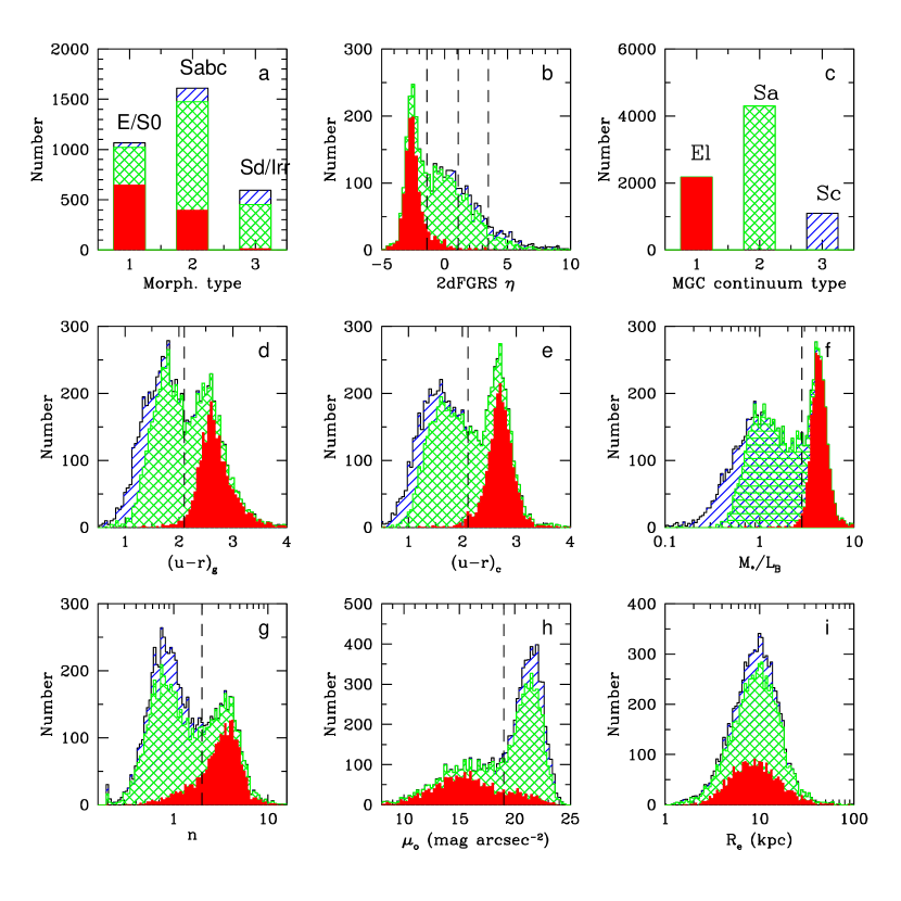
Figure 1: The various criteria by which the MGC can be subdivided (as indicated, see also Sections 2.1 – 2.8 ). The shading represents the location of MGC galaxies classified based on their continuum shape as either El (solid), Sa (hashed) or Sc (diagonal lines).

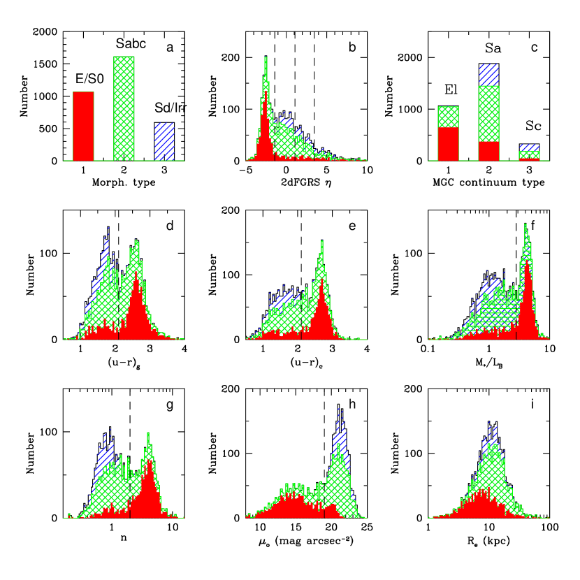
Figure 2: As for Fig. 1 except for galaxies with $B_{\mbox{\tiny\sc MGC}}<19$ mag only throughout. The shading now highlights how the eyebal morphological classifications into either E/S0s (solid), Sabcs (hashed) or Sd/Irrs (diagonal lines).

2.1 The MGC morphologies

We have derived the morphological classifications for the 3 314 galaxies that lie within the MGC size and surface brightness selection boundaries (see Driver et al., 2005) with $B_{\mbox{\tiny\sc MGC}}<19$ mag through eyeball classification (SPD). This is a subjective process and was achieved by visual inspection of batches of 20 grey scale images displayed over three surface brightness ranges: 19.0 – 26  mag arcsec^-2, 20.5 – 26  mag arcsec^-2, 22.0 – 26  mag arcsec^-2. The three visual classes are defined as follows:

$\bullet$ E/S0: Smooth, highly concentrated symmetrical systems with no obvious spiral-arm disc component.

$\bullet$ Sabc: Clear two-component bulge-disc system, generally smooth and symmetrical.

$\bullet$ Sd/Irr/Pec: Disc only (i.e., no obvious single core), asymmetric, highly disturbed or multiple-core systems.

These classifications are consistent with our deeper Hubble Space Telescope studies of more distant galaxies (Driver et al., 1995a, 1995b, 1998, 2003; Driver, 1999; Odewahn et al., 1996; Cohen et al., 2003), which are based on comparable physical resolution and signal-to-noise data. The entire classification process was undertaken by SPD over a period of some weeks and repeated several times until no reclassifications were necessary. Fig. 3 shows representative examples of each class including stars (see Liske et al., 2003 for details of the star-galaxy separation). Note that images of both red and blue ’ellipticals’ are shown and these are discussed in Section 3.2. Table 1 contains the morphological number counts which can be compared to our earlier and deeper HST studies listed above.

Table 1: Morphological number-counts from the MGC.

$B_{\mbox{\tiny\sc MGC}}$ (mag)	log N[All]	log N[E/S0]	log N[Sabc]	log N[Sd/Irr]
13.75	-1.012	-1.188	-1.489	—
14.25	-0.790	-1.489	-1.012	-1.489
14.75	-0.489	-1.012	-0.644	—
15.25	-0.343	-0.790	-0.586	-1.489
15.75	0.123	-0.535	-0.074	-0.711
16.25	0.396	-0.127	0.200	-0.790
16.75	0.677	0.226	0.373	-0.147
17.25	0.894	0.385	0.640	0.015
17.75	1.228	0.717	0.911	0.547
18.25	1.474	0.978	1.143	0.802
18.75	1.686	1.213	1.357	0.974
19.25	1.901	—	—	—
19.75	2.122	—	—	—

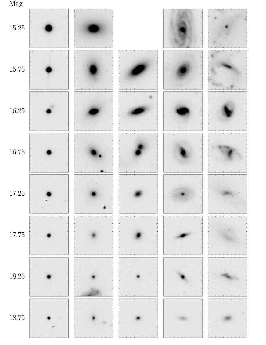
Figure 3: A random sample of our postage stamp images for representative examples of (left to right) stars, red ellipticals, blue ellipticals (dEs?), spirals, and late-type irregulars at various magnitude intervals (as indicated). Faintwards of $B_{\mbox{\tiny\sc MGC}}=19$ mag morphological classification becomes intractable and higher-resolution data in better seeing is required.

2.2 The 2dFGRS $\eta$ parameter

The 2dFGRS $\eta$ parameter is defined in Madgwick et al. (2002) and is a linear combination of PC1 and PC2 from a Principle Component Analysis of the spectra. PC1 contains information on the emission and absorption line strengths and the continuum (with roughly equal weights) and PC2 contains information on just the line strengths. The linear combination maximises line features and hence provides a good indicator of current and previous star-formation. The reader is referred to fig. 7 of Madgwick et al. (2002) for canonical examples of $\eta$ type 1, 2, 3, & 4 spectra.

2.3 MGC continuum classification

We divide the sample into three MGC continuum types using our spectral template fitting code (see Driver et al., 2005) and restricting it to fit either a 15 Gyr elliptical (El), a 7.4 Gyr early-type spiral (Sa) or a 2.2 Gyr late-type spiral (Sc). All three continuum spectra are taken from Poggianti (1997). Fig. 4 shows both the location of the broad band filters and our three canonical continuum shape spectra shifted to $z=0.1$. The optimal fitting spectrum for each galaxy is obtained as described in Driver et al. (2005). In brief, the flux for the $uBgriz$ filter set is derived for each template at the known redshift of the object and $\chi^{2}$-minimisation used to determine the best fitting template (where the normalisation is marginalised over). Where no satisfactory fit is found the filters are dropped in the order of $B_{\mbox{\tiny\sc MGC}}$ (non-SDSS), then $u$ (red leak) and then $z$ (fringing). The optimal spectra provide an indication of the continuum shape. In essence the MGC continuum typing is simply a sophisticated colour cut whioch uses all available colours hence correlation between continuum type and colours is to be expected.

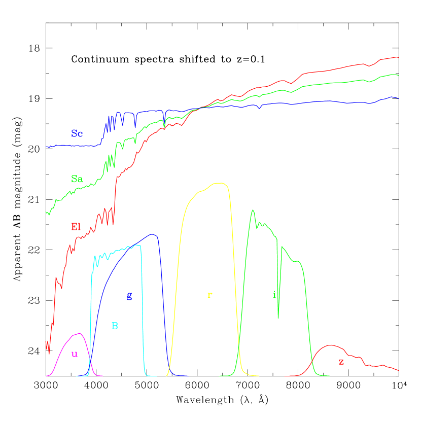
Figure 4: The three adopted continuum spectra used in our fitting process. The spectra are shifted to a redshift of 0.1 and are arbitrarily scaled. We also show the transmission curves of the filters for which photometry is available.

2.4 SDSS global and core colours

Overlap with the SDSS-DR1 enables complimentary $ugriz$ photometry for 99% of the MGC galaxy sample (see Cross et al., 2004). To convert these colours to rest-wavelengths we use the appropriate spectral template and a simple evolutionary recipe as described in Driver et al. (2005). The SDSS-DR1 colour bimodality was first reported by Strateva et al. (2001) and studied in more detail by Baldry et al. (2004). Its environmental dependency was explored further in Balogh et al. (2004a). These studies typically adopted the global $(u-r)$ rest colour. Here we show both the global and the core $(u-r)$ rest colours (hereafter $(u-r)_{g}$ and $(u-r)_{c}$ respectively). The former is derived from Petrosian magnitudes and the latter from PSF magnitudes. One may argue whether the core-colour is better defined by the PSF magnitude, by a minimal fixed aperture colour, or even fibre magniutdes which are degraded to a consistent poor seeing value. Clearly, PSF magnitudes are more appropriate for ultra-compact sources, and a fixed aperture slightly larger than the seeing more appropriate for extended sources. However as the cores are often barely resolved we essentially opt for the smallest credible measurement which is the PSF magnitude. While this is somewhat profile dependent an equivalently small fixed aperture would be biased by the wavelength dependency of the PSF size. Both of the colour distributions are seen to be strongly bimodal (see Fig. 1d and 1e, respectively) with the peaks marginally better separated in the $(u-r)_{c}$ distribution. We separate the galaxy population into two classes with cuts at $(u-r)_{g}=2.1$ and $(u-r)_{c}=2.35$ respectively.

2.5 Stellar mass-to-light ratios

Bell & de Jong (2001) provide a standard prescription to determine stellar masses and stellar mass-to-light ratios from broad band colours. From their Table 1 we have:

$\log(M^{*}/L_{B})=-1.224+1.251(B-R)$.

From Cross et al. (2004) we have the following conversions from SDSS-DR1 photometry of:

$(B-R)=1.54(g-r)+0.35$,

and can recast the above as:

$(M^{*}/L_{B})=10^{[{1.93(g-r)-0.79}]}$,

where $M^{*}/L_{B}$ is the $B_{\mbox{\tiny\sc MGC}}$ stellar mass-to-light ratio in solar units. We elected to use the SDSS-DR1 colours for consistency rather than $(B_{\mbox{\tiny\sc MGC}}-r)$ because the differing deblending algorithms occasionally lead to spurious ($B_{\mbox{\tiny\sc MGC}}-r)$ colours. Not surprisingly, as the stellar mass-to-light ratios are derived directly from the global-$(g-r)$ colour, we again see (Fig. 1f) a bimodality with an obvious division at $\log(M^{*}/L_{B})=0.45$.

2.6 The MGC Sérsic indices

The MGC Sérsic profile indices ($n$), are derived using GIM2D (Simard et al., 2002) and the process is described in detail in Allen et al. (2005). Briefly, GIM2D performs a $\chi^{2}$-minimisation between the image and a 6-parameter model image. A segmentation mask derived from SExtractor is used to indicate which pixels are associated with the object, and an appropriate PSF image is convolved with the model image. The software uses the standard Sérsic profile (Sérsic, 1963, Graham & Driver, 2005) returning the total flux, Sérsic index ($n$), half-light radius ($R_{e}$), ellipticity, position angle and positional and background offsets. Fig. 1g shows the distribution of the best-fitting Sérsic parameters for the MGC. The distribution in $\log(n)$ is bimodal, presumably reflecting bulge dominated (i.e., pressure supported) or disc dominated (i.e., rotationally supported) systems. Note that it is more appropriate to plot $\log(n)$ rather than $n$, as $n$ appears in the exponent of the intensity equation, i.e., a small change in $n$ makes a large difference for low $n$ values but minimal difference for high-$n$ values. We adopt a division at the saddle point of $n=2.0$. From repeat observations of $702$ objects we have quantified the random error on the Sérsic index to be $\Delta\log(n)=\pm 0.041$.

2.7 The MGC central surface brightnesses

The (extrapolated) central surface brightness ($\mu_{0}$) is calculated directly from the GIM2D Sérsic only fits and hence strongly dependent (although not exclusively) on the Sérsic index. It is included here for completeness as many earlier studies have subdivided the population by a surface brightness cut. The distribution is bimodal and we divide the galaxy population at $\mu_{0}=19~{}B_{\mbox{\tiny\sc MGC}}$  mag arcsec^-2. Note that in our previous studies ( Cross et al., 2001; Cross & Driver, 2002; Driver et al., 2005) we explored the effective surface brightness absolute magnitude plane. The distinction is important, whereas bulges and discs typically have similar effective surface brightnesses their central surface brightnesses are significantly different. For overcoming selection bias the former is more relevant, for exploring variations the latter is more appropriate.

2.8 The MGC half-light radii

The half-light radius ($R_{e}$), is calculated directly by the GIM2D code and is therefore PSF-corrected. The distribution is relatively broad and peaked at around $10$ kpc. Hence, while bimodalities exist in many observable properties, the size distribution is smooth (and hence the effective surface brightness as well). There is no obvious location at which to divide the population.

2.9 The observed (uncorrected) distributions

Fig. 1 shows the observed distributions, i.e., uncorrected for volume bias, for galaxies with $B_{\mbox{\tiny\sc MGC}}<20$ mag and $M_{B_{\mbox{\tiny\sc MGC}}}-5\log h<-16$ mag, except for morphological type and $\eta$ which are only known to $B_{\mbox{\tiny\sc MGC}}=19$ mag. Note that the absolute magnitude limit essentially confines this study to the giant galaxy regime (with some contribution from the brightest dwarf ellipticals). In Fig. 2 the overall distributions also shown subdivided according to MGC continuum type (solid, El; hashed, Sa; or diagonal lines, Sc). This highlights the correlated nature of the bimodalities. However, it is also clear that the subdivisions of the galaxy population based on colour, morphological type, etc., will each extract distinct subsets of the galaxy population. Hence, great care must be taken when comparing high and low redshift samples subdivided by different methods. Fig. 2 shows the same distributions but restricted to the $B_{\mbox{\tiny\sc MGC}}<19$ mag population. The morphological groups (E/S0, Sabc, Sd/Irr) are shown with distinctive shading throughout (solid, hashed, diagonal lines, respectively). From Fig. 2 it is clear that the E/S0 (bulge-dominated) and Sd/Irr (disc-only) populations occupy the extremes of the bimodal distributions with the Sabc distribution as a bridging population.

Figure 5: (main panel) the global $B$-band luminosity function derived via our modified step-wise maximum likelihood method for the $B_{\mbox{\tiny\sc MGC}}<19$ (solid squares and solid line) and $B_{\mbox{\tiny\sc MGC}}<20$ (open circles and dotted line) mag samples. (upper right) the 1,2 and 3 $\sigma$ error-ellipses of the Schechter function fits and (lower right) the luminosity surface brightness plane and the logarithmic contours for the $B_{\mbox{\tiny\sc MGC}}<19$ (dotted line) and $B_{\mbox{\tiny\sc MGC}}<20$ mag (solid line) samples. The two dashed lines denote the limits of reliability for the two samples.

3 The luminosity distributions and Schechter functions

To obtain luminosity distributions for sub-populations we first re-derive the global bivariate brightness distributions for the $B_{\mbox{\tiny\sc MGC}}<19$ mag and $B_{\mbox{\tiny\sc MGC}}<20$ mag samples following Driver et al. (2005). The method implemented in Driver et al. (2005) is a variant of the standard step-wise maximum likelihood (SWML; see Efstathiou et al., 1988) operating in the plane of luminosity and surface brightness (as opposed to luminosity alone). The main advantage is the ability to track the five key selection boundaries (see Driver, 1999) which govern whether a galaxy is reliably detected or not: maximum/minimum luminosity, maximum/minimum size, and maximum mean effective surface brightness. The analysis assumes ($\Omega_{M}=0.3,\Omega_{\Lambda}=0.7$) with $H_{o}=100$h km s^-1Mpc^-1 and K-corrections derived individually for each galaxy (see Driver et al., 2005 for specific details). Fig. 5 shows a comparison of the luminosity distributions, functions, error ellipses and LSP distributions for these two samples which are fully consistent with each other.

To derive the subdivided luminosity distributions, $\psi(M,x)$ we now simply calculate:

$$\psi(M,x)=\sum_{\mu=-\infty}^{\mu=\infty}[f_{x}(M,\mu).\phi(M,\mu)]\delta\mu,$$ (1)

where $f_{x}(M,\mu)$ represents the apparent frequency of some attribute, $x$, (e.g., fraction of E/S0 type) within that absolute magnitude and surface brightness bin, $\delta M\delta\mu$. $\phi(M,\mu)$ represents the space density of all galaxies in that same interval. The integral over surface brightness then converts the bivariate distribution to the monovariate luminosity function; note that although the integral ranges across all values of surface brightness the distribution at any $M$ is actually bounded by the selection limits. This is essentially identical to re-deriving the LSP (also known as the bivariate brightness distribution or BBD, see Boyce & Phillipps, 1995) for each sub-population but computationally simpler and more stable. Figs. 6–9 show the recovered luminosity distributions for the various subdivisions. In each case the luminosity distributions were fitted by a Schechter function to $M_{B_{\mbox{\tiny\sc MGC}}}-5\log h=-16$ mag. In each figure the recovered data are shown (left) along with the best Schechter function fits and the 1-,2- and 3- $\sigma$ error contours (right-side). The fitting parameters are also tabulated in Table 2 along with the 1-$\sigma$ errors from the $\chi^{2}$ fit, the integrated luminosity density ($j_{b_{j}}$), the median $(u-r)_{g}$ and the total stellar mass for each subdivision. The luminosity densities and stellar densities $(M^{*})$ were derived as follows:

$j_{b_{j}}=\phi^{*}10^{-0.4(M_{B}-M_{\odot})}\Gamma(\alpha+1)$,

and,

$M^{*}=\sum_{i}^{N}10^{[{1.93(g-r)-0.79})}10^{-0.4(M_{B}-M_{\odot})}$.

i.e., analytically for the luminosity density and an empirical sum for the stellar mass density because of the strong colour dependency.

3.1 Luminosity distributions/functions by morphological type

In Fig. 6 (upper) we show the eyeball morphological luminosity distributions/functions. Although the three divisions show segregation in their Schechter function parameters, the distinction between the E/S0 and Sabc categories is not particularly strong. Certainly the E/S0s do not appear to follow the Gaussian distribution anticipated by Binggeli et al. (1988), reported in Jerjen & Tammann (1997), and discussed extensively in de Lapparent (2003). In Ellis et al. (2005, their fig. 3) we found that our eye was often fooled by smooth, blue, low-luminosity spheroidal systems. This highlighted both the subjective nature of eyeball classification and its susceptibility to variations in data quality. Whether the blue spheroid population constitutes the tail-end of the ’downsizing’ phenomenon or interlopers is at this stage unclear but under investigation. If one uses additional colour information to separate out the blue and red spheroids (i.e., following Ellis et al.) and re-derives the morphological luminosity distributions we now get the distributions shown in Fig. 6 (lower). The luminosity distribution of the blue spheroid (BS) population alone (not shown but see Table 2) follows almost exactly the same distribution shape as the Sd/Irr population and most likely has a common origin. This is also consistent with the idea that the E/S0 population has indeed been contaminated by a population of smooth blue dwarf systems (dwarf spheroidals). In so far as a comparison can be made, our values could be contrasted to those listed in Table 4 of de Lapparent (2003) where we see measurements for the E/S0 class from the Stromlo APM survey ($M^{*}_{B_{\mbox{\tiny\sc MGC}}}=-19.33$ mag, $\alpha=+0.2$; Loveday et al., 1992), the Southern Sky Redshift Survey 2 ($M^{*}_{B_{\mbox{\tiny\sc MGC}}}=-19.64$ mag, $\alpha=-1.00$; Marzke et al., 1998) and the Nearby Optical Galaxy Sample ($M^{*}_{B_{\mbox{\tiny\sc MGC}}}=-19.80$ mag, $\alpha=-0.97$; Marinoni et al., 1999). These three surveys concur well with our uncontaminated and contaminated E/S0 samples suggesting the problem of BS contamination may be endemic in all eyeball classified samples (and hence in ANN classification as well) – see Ellis et al. (2005) for the formal detection of these systems and also Cross et al. (2004) for discussion of BS contamination of field ellipticals at $z\sim 0.75$ (r.f., fig.2a from Bell et al., 2005). While arguably a combined eye and colour cut may provide a more robust division, the process of morphological classification (whether by eye or ANN) is subjective and hence susceptible to confusion, controversy and ambiguity.

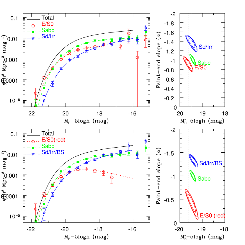
Figure 6: (upper) The derived data and fitted Schechter functions subdivided by morphological type and (lower) with the blue spheroids (BS) moved into the Sd/Irr category.

3.2 Luminosity distributions/functions by $\eta$ and MGC continuum type

Fig. 7 shows the luminosity distributions/functions subdivided by $\eta$ (upper) or MGC continuum type (lower). The luminosity distributions/functions subdivided by $\eta$ type concur with the earlier results by the 2dFGRS team (i.e., Folkes et al., 1999; Madgwick et al., 2002), with the $\eta 1$-type showing a distinct luminosity distribution and less distinction between the remaining $\eta$ types. Unfortunately the fraction of galaxies without a known $\eta$ type is significant (even to $B<19$ mag) due to the requirement for moderately good signal-to-noise spectra.

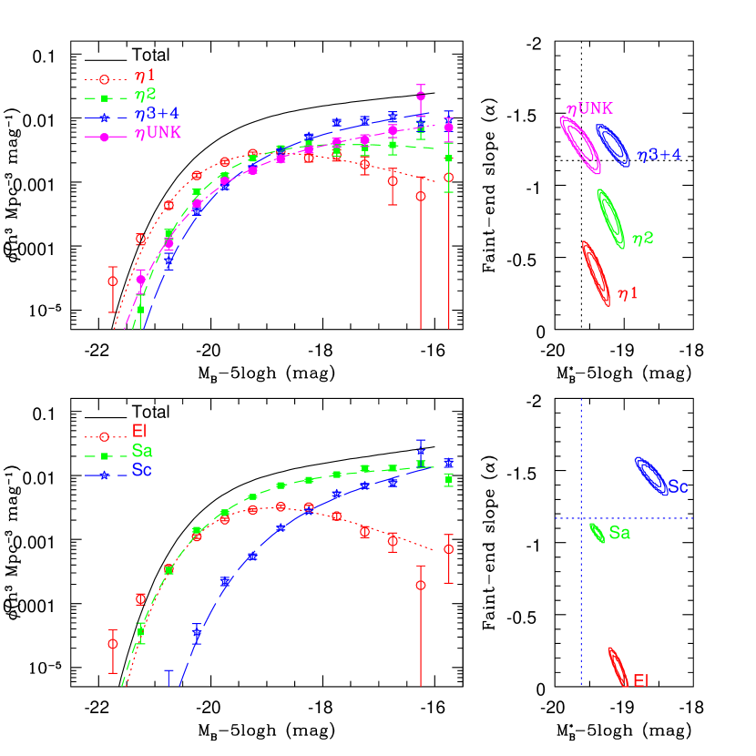
Figure 7: (upper) The derived data and fitted Schechter functions subdivided by 2dFGRS-$\eta$ parameter and (lower) subdivided by MGC continuum type.

Our continuum typing, based on spectral template fitting to the available $uBgriz$ broad-band photometry, appears significantly more promising with the three continuum shapes (see Fig. 4) represented by very distinct luminosity distributions/functions. From Fig. 1 we see that these distinctions (shown as shaded, hashed and lines histograms) are well correlated with other observables. While correlation between continuum type and colour (and hence stellar mass-to-light) is to be expected, the correlation with structural measurements is significant as no structural information was used in the determination of the MGC continuum type. The El continuum type extracts the red, high mass-to-light ratio, concentrated, and predominantly luminous systems. The Sa class exhibits a broader range bridging the El and Sc populations. The Sc class constitutes the bluest and least concentrated systems. The implication is that the El systems are luminous (massive) and old (or at least their stars are), and the Sc systems appear to be predominantly low luminosity (low mass), and young (late-formers).

3.3 Luminosity distributions/functions by colour and mass-to-light ratio

Fig. 8 shows the luminosity distributions/functions subdivided by $(u-r)_{g}$ (upper) and $(u-r)_{c}$ colours (lower). It is worth noting that our calculation of the rest colour is independent of the standard SDSS method, based on our own spectral template fitting routine which includes all 27 spectral templates given by Poggianti (1997), see Driver et al. (2005) for details. The luminosity distributions of the red and blue populations are significantly distinct. Worth noting is that the $(u-r)_{c}$ colour – derived from SDSS-DR1 PSF magnitudes – appears to segregate galaxies better than the global colour – derived from SDSS-DR1 Petrosian magnitudes. The improvement in segregation (see Fig. 8 right side panels) is significant and could be interpreted as better separating the galaxy population into those with dominating old bulges and those without. The key question is why do red bulges predominantly occur in luminous galaxies? Presumably either the low-luminosity bulges are unresolved and hence hidden within the PSF, or that old inert (and therefore red) low-luminosity bulges are rare. This is consistent with some studies which argue that the bulges of late-type systems are pseudo-bulges built up through inner disc and bar instabilities (e.g., Erwin et al., 2003) rather than genuine bulges. As genuine bulges should be cuspier one might expect the core colour to be better at identifying such systems. As mentioned in Section 2.4 our core colour is not ideal but simply relies on the colour within the smallest available aperture. An obvious extension would be to derive the core colour from multicolour 2D bulge-disc decomposition models to see whether the red peak becomes even sharper.

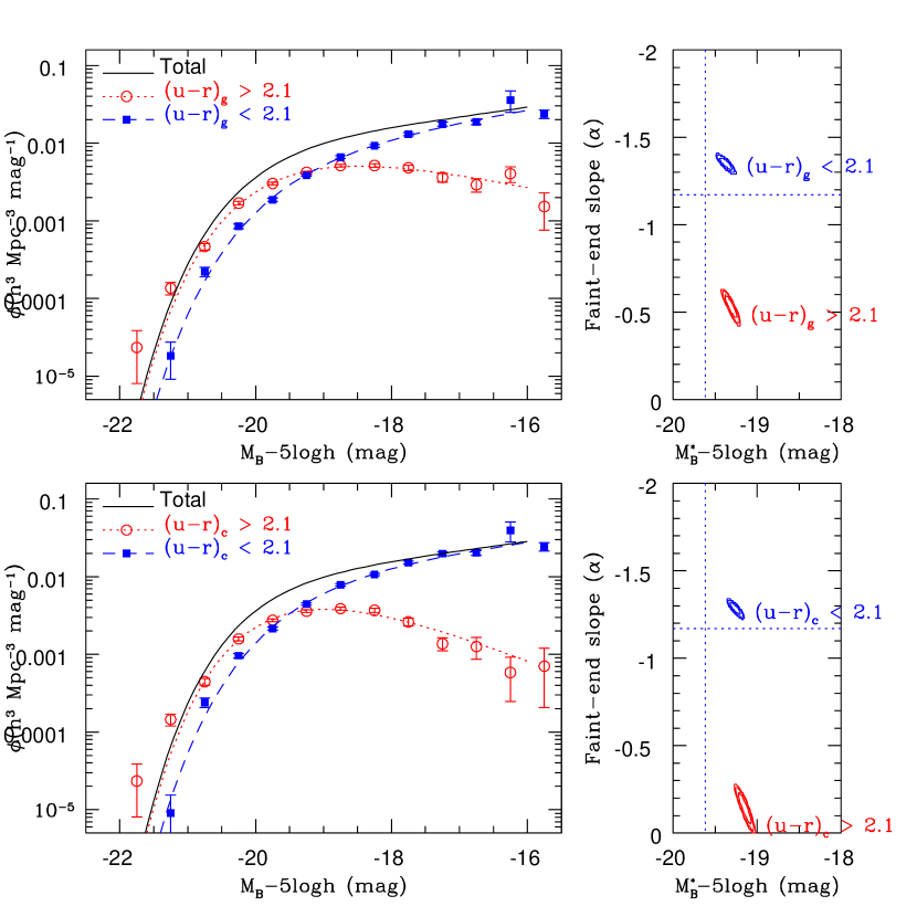
Figure 8: The derived data and fitted Schechter functions subdivided by $(u-r)_{g}$ colour (upper) and $(u-r)_{c}$ colour (lower)

The SDSS $(u-r)_{g}$ colour bimodality was studied in detail by Baldry et al. (2004) who derived the $r$-band luminosity functions and identified faint-end parameters of $\alpha=-1.35\pm 0.05$ and $\alpha=-0.83\pm 0.002$ for the blue and red populations respectively. This compares with our values of $\alpha=-1.35\pm 0.02$ and $\alpha=-0.54\pm 0.05$ for our $B$-band selected samples. As one expects a $B$-band sample to preferentially miss red systems when compared to an $r$-band sample, the higher $\alpha$ for the red systems is unlikely to be significant. As the mass-to-light ratios are derived from the global $(g-r)$ colour (via Bell & de Jong, 2001) the narrowness of the mass-to-light ratio distribution is expected. However, the MGC continuum classification appears remarkably robust at identifying systems occupying the high mass-to-light ratio peak (Fig. 1f). Perhaps even more interesting is the extreme narrowness of the high-M/L peak, essentially a representation of the well known colour-magnitude relation of cluster ellipticals (Sandage & Visvanathan, 1978). This narrowness presumably reflects the universal endpoint of galaxy evolution, which in turn places a joint constraint on the age, metallicity and even the universality of the IMF (see Bruzual & Charlot, 2003).

3.4 Luminosity distributions/functions by structure

Fig. 9 shows the luminosity distributions/functions subdivided by Sérsic index, $n$ (upper), and central surface brightness (lower). As the central surface brightness is derivable from $n$, total magnitude and effective radius, it is not independent and hence the similarity in the two distributions (upper and lower panels) is to be expected. Taking the $\log(n)$ division we see that while the high and low-$n$ populations follow distinct luminosity distributions, the distinction is not as great as for the MGC continuum and colour divided distributions. This is, at least in part, due to the fact that some dEs with $-16>M_{B_{\mbox{\tiny\sc MGC}}}-5\log h>-18$ mag will have $n<2$ and others will have $n>2$. Folding in colour information to separate the red dEs from the blue discs will help and is considered in the following section.

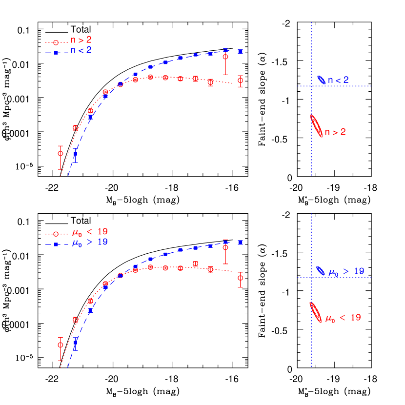
Figure 9: The derived data and fitted Schechter functions subdivided by $\log($Sérsic index$)$ (upper) and fitted central surface brightness (lower).

3.5 Luminosity distribution summary

The main conclusions from this section are:

(1) Morphological classification based on the eye, including Artificial Neural Networks which use a training set, are fraught with difficulty because of the subjective nature of the classification process.

(2) In so far as morphological luminosity functions can be obtained, particular care must be taken to distinguish genuine ellipticals from smooth, blue, low-luminosity systems and eyeball classifications should be made using colour images if possible.

(3) Both global and core $(u-r)_{g,c}$ colours segregate the population well into blue and predominantly luminous red systems.

(4) The core colour appears to better segregate the two populations (in $M-\alpha$-space) than the global colour, probably due to the blending of colours from red bulges embedded in blue discs.

(5) The narrowness of the red, core-colour peak may imply an early formation age from a universal initial mass function for these systems (as commonly assumed, e.g., Bell & de Jong, 2001).

(6) Further gains may be made by moving beyond a single colour cut to a continuum-type classification system based on multiple colours. This highlights three distinct populations. A luminous red population a low luminosity blue population and an intermediate population, these are closely associated with E/S0 (bulge-dominated), Sd/Irr (disc-only) and Sabc (bulge and disc) systems.

(7) Galaxies can also be effectively separated into two populations using structural division in $\log(n)$ space. The populations constitute a concentrated and diffuse population.

(8) Colour appears to segregate the galaxy population more effectively than any other single measurement (i.e., Sérsic index or surface brightness).

In the next section we continue the analysis by exploring selected bivariate distributions.

4 Bivariate distributions

We derive volume corrected bivariate distributions/functions in a similar manner to the luminosity distributions by starting from the overall bivariate brightness distributions for the entire $B_{\mbox{\tiny\sc MGC}}<19$ and $B_{\mbox{\tiny\sc MGC}}<20$ mag population and projecting attributes $x$ and $y$ on to a new plane, i.e.,

$$\psi(x,y)=\sum_{M_{B_{\mbox{\tiny\sc MGC}}}=-\infty}^{M_{B_{\mbox{\tiny\sc MGC}}}<-16}~{}~{}\sum^{\mu=+\infty}_{\mu=-\infty}f_{x,y}(M,\mu).\phi(M,\mu)\delta M\delta\mu,$$ (2)

where the values are defined as for Eqn. (1). Fig. 10–14 show the bivariate distributions of: $(u-r)_{g}$, $(u-r)_{c}$, $\log(n)$, $\mu_{0}$ and $\log(R_{e})$ versus $M_{B_{\mbox{\tiny\sc MGC}}}$. For each figure we show (upper left) the raw observed distribution as both data points and contours, and (lower left) the volume corrected distributions using Eqn. (2). The right-side panels show the histograms along the absolute magnitude axis. As a reminder, only galaxies with $M_{B_{\mbox{\tiny\sc MGC}}}-5\log h<-16$ mag are included in the analysis.

4.1 Bivariate distributions by colour

Figs. 10 and  11 show the bivariate distributions of rest $(u-r)_{g}$ and $(u-r)_{c}$ colours versus $M_{B_{\mbox{\tiny\sc MGC}}}$. In both figures we see a distinct red and blue sequence as characterised by Baldry et al. (2004) using SDSS data. In both figures the red distribution appears entirely bounded albeit overlapping with the luminous end of the more extensive blue population. Both the red and blue sequences show colour gradients reminiscent of the luminosity-metallicity relation seen in nearby rich clusters. Note that bimodality is only obvious in the observed histograms and not in the volume corrected histograms as the numbers are dominated by the lower luminosity systems. In terms of stellar mass (not shown) the bimodality remains but is skewed towards the red peak. The division between the red and blue populations is more distinct (and the red peak histogram narrower) when $(u-r)_{c}$ colour is used. This implies that the core colour is the more fundamental (less contaminated) measure. Further data probing to lower luminosities is required to unequivocally conclude that the red sequence is bounded at low luminosity (i.e., few galaxies with $(u-r)_{c}>2$ and $M_{B_{\mbox{\tiny\sc MGC}}}-5\log h<-17$ mag). An indication of a low luminosity red spike (dEs ?) is seen but with extremely low significance because of limited statistics and the large volume amplification at the faint-end.

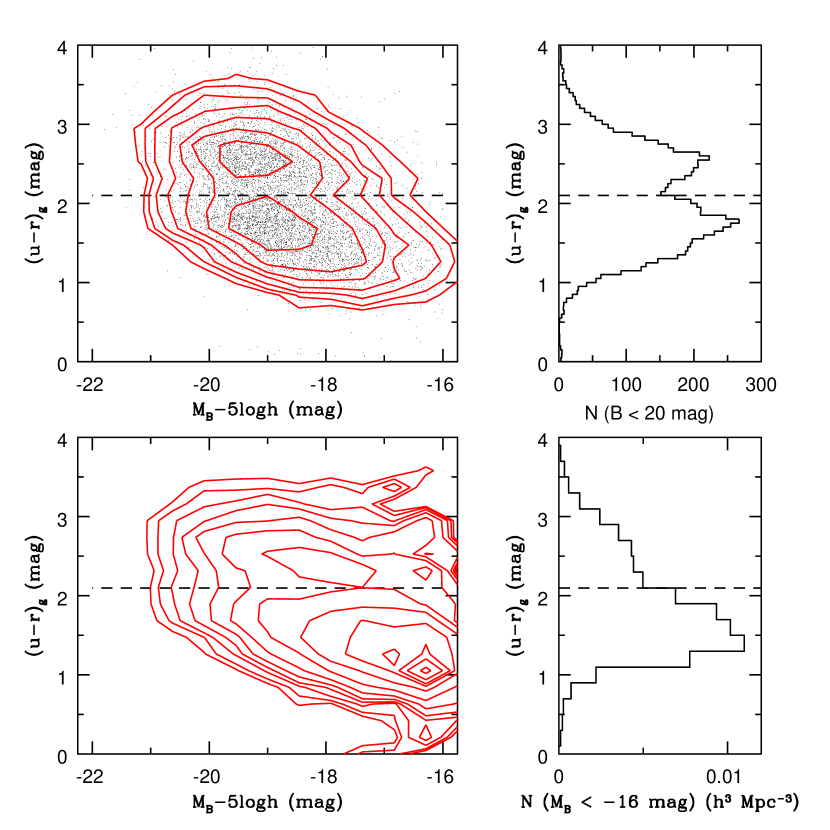
Figure 10: (upper left) the observed $(u-r)_{g}$ versus $M_{B_{\mbox{\tiny\sc MGC}}}$ distribution (dots and 0.2 dex contours) and histogram (upper right). (lower left) the volume-corrected $(u-r)_{g}$ versus $M_{B_{\mbox{\tiny\sc MGC}}}$ distribution (dots and 0.2 dex contours) and histogram (lower right).

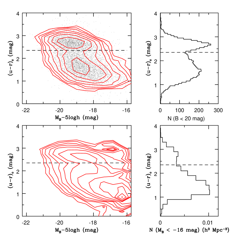
Figure 11: (upper left) the observed $(u-r)_{c}$ versus $M_{B_{\mbox{\tiny\sc MGC}}}$ distribution (dots and 0.2 dex contours) and histogram (upper right). (lower left) the volume-corrected $(u-r)_{c}$ versus $M_{B_{\mbox{\tiny\sc MGC}}}$ distribution (dots and 0.2 dex contours) and histogram(lower right).

4.2 Bivariate distributions by structure

Figs. 12, 13 and 14 show the corresponding structural bivariate distributions for $\log(n)$, $\mu_{0}$ and $R_{e}$ respectively. The first two show bimodality albeit less obviously than for the global and core-colour distributions. Both Figs. 12 and 13 suggest a concentrated, high surface brightness, low-luminosity population close to the limit of analysis (in the volume corrected distributions). Whether this represents a third distinct population or a manifestation of the limiting statics close to the selection boundaries is difficult to establish and requires additional data to clarify. One clear possibility is that it may represent the onset of nucleated dwarf systems which would exhibit both higher than typical Sérsic indices and correspondingly higher central surface brightnesses. Unlike the colour bivariate distributions, the distinct concentrated giant (E) distribution blends into the diffuse (low-$n$, disc) population towards lower luminosities. The size distribution shows no bimodality but a broadening towards lower luminosity as found by Shen et al. (2003) and Driver et al. (2005).

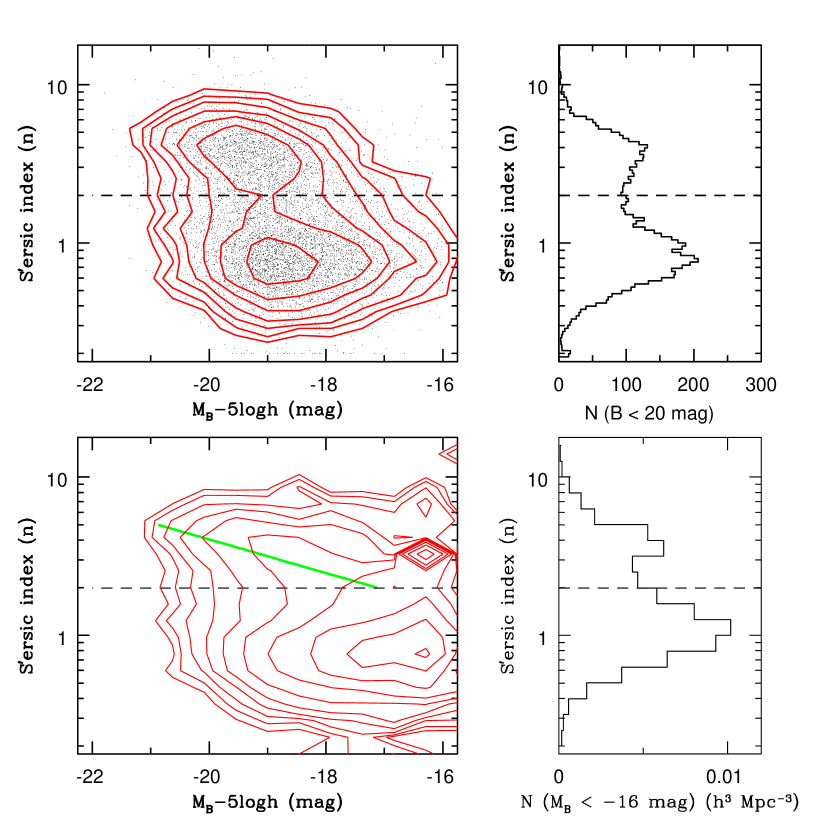
Figure 12: (upper left) the observed $\log(n)$ versus $M_{B_{\mbox{\tiny\sc MGC}}}$ distribution (dots and 0.2 dex contours) and histogram (upper right). (lower left) the volume-corrected $\log(n)$ versus $M_{B_{\mbox{\tiny\sc MGC}}}$ distribution (dots and 0.2 dex contours) and histogram (lower right). The solid line shows the known relation for spheroids (see Graham & Guzmán 2003).

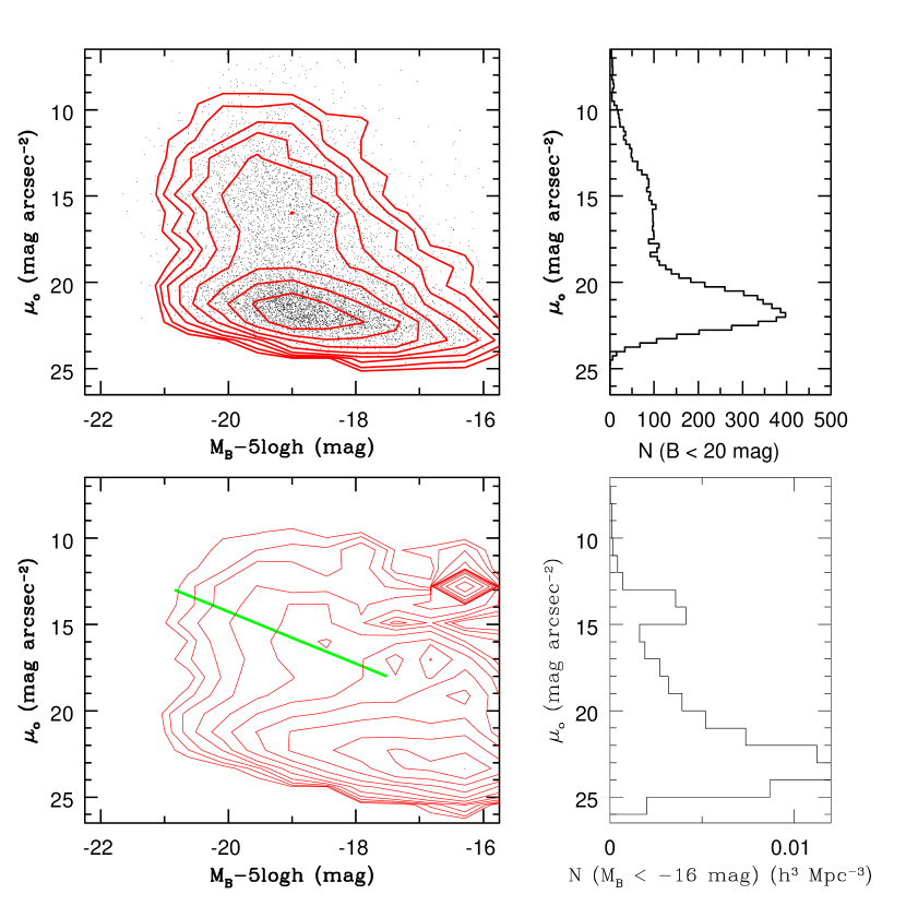
Figure 13: (upper left) the observed $\mu_{o}$ versus $M_{B_{\mbox{\tiny\sc MGC}}}$ distribution (dots and 0.2 dex contours) and histogram (upper right). (lower left) the volume-corrected $\mu_{o}$ versus $M_{B_{\mbox{\tiny\sc MGC}}}$ distribution (dots and 0.2 dex contours) and histogram (lower right). The solid line shows the known relation for spheroids (see Graham & Guzmán 2003).

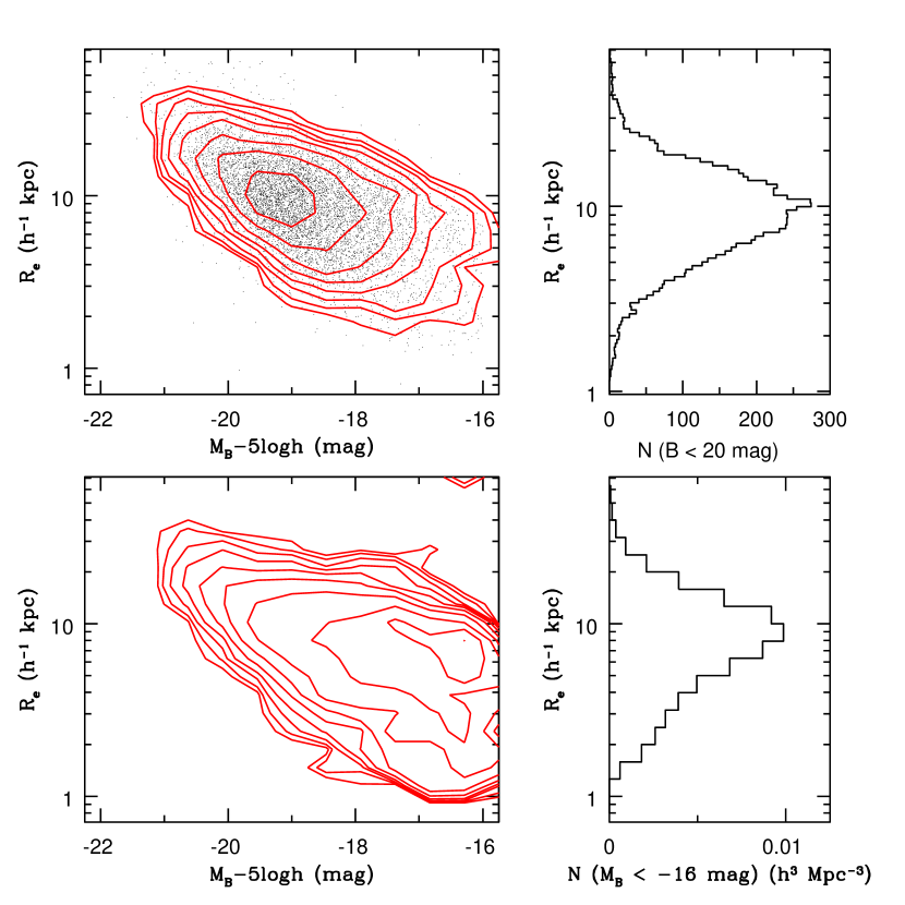
Figure 14: (upper left) the observed HLR versus $M_{B_{\mbox{\tiny\sc MGC}}}$ distribution (dots and 0.2 dex contours) and histogram (upper right). (lower left) the volume-corrected HLR versus $M_{B_{\mbox{\tiny\sc MGC}}}$ distribution (dots and 0.2 dex contours) and histogram (lower right).

4.3 The joint distribution of core-colour and Sérsic index

Having established that bimodality exists in both the colour and $\log(n)$ distributions, and that the $(u-r)_{c}$ shows the bimodality most strongly, we now explore the joint $(u-r)_{c}$-$\log(n)$ plane. Fig. 15 shows the observed distribution (upper) in contour form (left) and as a 3D projection (right). The lower panels show the equivalent for the volume corrected distribution. Fig. 15 shows two distinct peaks with a bridge between them pointing towards either two distinct populations or two dominant characteristics. The peaks are typified by a high Sérsic index red peak and a low Sérsic index blue peak. Note that the additional third spike (in the lower right panel) may constitute a compact blue population reminiscent of the blue spheroids (see Section 3.1). The key question at this stage is whether we are seeing two distinct galaxy populations (red and blue) or whether the peaks correspond to two characteristics (i.e., bulges and discs). Bulge-disc decomposition is clearly essential to establish this unambiguously. However early indication comes from the morphological classifications where, by definition (see Section 2.1), E/S0s represent bulge-dominated systems, Sabcs joint bulge-disc systems and Sd/Irrs disc-only systems. Fig. 16 (left) shows the raw observed distributions (i.e., equivalent to Fig. 15 [upper right]) for the E/S0 (upper), Sabc (middle) and Sd/Irr (lower) populations. We see quite clearly that the bulge-dominated (E/S0) and disc only (Sc) systems lie almost exclusively in one peak or the other. The bulge+disc systems (Sabcs) straddle both peaks and the divide. This is extremely strong evidence that points towards the fundamental nature of bulges and discs and the need to interpret colour bimodality as a manifestation of two components rather than two distinct galaxy populations. Note that we have shown the original E/S0 classifications without the additional colour tinkering described in Section 3.1 and the BS population shows up as fairly distinct and lying within the blue peak. Fig. 16 (right) shows the observed distributions for the MGC continuum classifications of El (upper), Sa (middle) and Sc (lower). This suggests that while the El–Sa division is fundamental the Sa–Sc division is probably not, but instead merely an arbitrary cut of a continuous distribution.

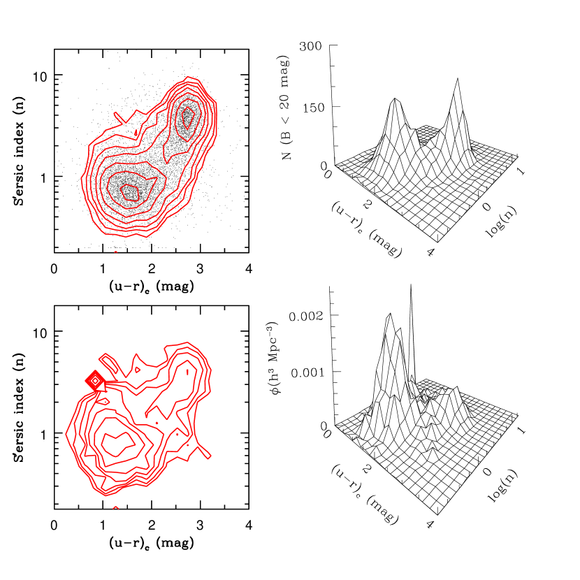
Figure 15: (upper) the observed distribution of log(n) versus $(u-r)_{c}$ colour (left, shown as data points and 0.2 dex contours; right shown as a 3D plot with the z-axis linear). (lower) the volume corrected distribution of $\log(n)$ vs $(u-r)_{c}$ colour (left, shown as 0.2 dex contours and right as a 3D plot with z-axis linear).

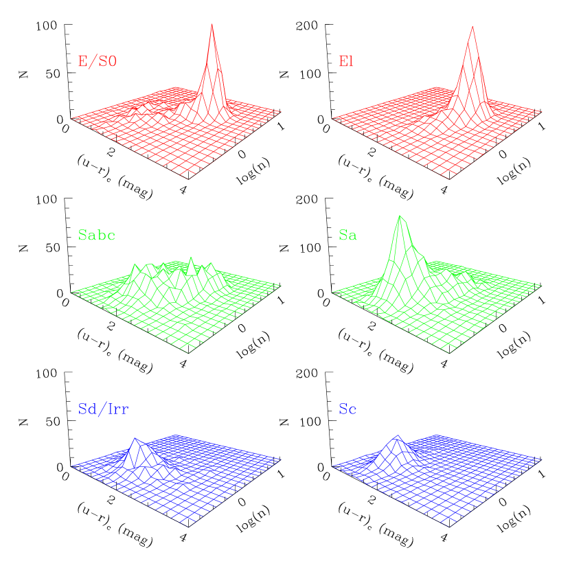
Figure 16: (left side) The distribution of E/SO (upper), Sabc (centre) and Sd/Irrs (lower) in the $\log(n)$ vs $(u-r)_{c}$ colour. (right side) The distribution of el (upper), Sa (centre) and Sc (lower) in the $\log(n)$ vs $(u-r)_{c}$ colour

5 Discussion

Our main result is that bimodality occurs in both the rest-$(u-r)$ and $\log(n)$ distributions and Fig. 15 highlights the 2D nature of this bimodality with two peaks of approximately equal height and shape in the observed ($M_{B_{\mbox{\tiny\sc MGC}}}<-16$ mag) plane (upper). We have argued in the previous section that these two peaks are best explained by the two component nature of galaxies, i.e., bulges and discs. Fig.17 shows how the stellar mass is distributed across the $(u-r)_{c}-\log(n)$ plane today, and the red concentrated peak is noticeably larger containing ($\sim 71\pm 6$) per cent of the total stellar mass. Spheriods (i.e., E/S0[red], c.f., Table 2) account for ($35\pm 2$) per cent. Systems with both bulges and discs must therefore account for the remaining 36 per cent. If one naively assumes a mean $B/T\sim 0.5\pm 0.2$, then this yields a total stellar mass content in spheroids and bulges of ($53\pm 7$) per cent. The discs hence make up the remaining ($47\pm 7$) per cent. Note that although we truncate our distributions at $M_{B_{\mbox{\tiny\sc MGC}}}-5\log h=-16$ mag, the luminosity functions are sufficiently flat to suggest a minimal contribution to the stellar mass density and therefore dwarf systems are negligible in terms of total stellar mass estimates (as also inferred in Driver, 1999).

The very narrow distribution of the red peak (see Figs 1 and 2) also implies a universal continuum shape which may only come about for old systems which formed with a universal IMF. Mergers which lead to bulges must either occur early or without significant star-formation i.e., dry-merging (see Graham, 2004; Faber et al., 2005 and Bell et al., 2005 for fairly stringent constraints on the level of dry-mergers at $z<1$). Hence it seems that around half of the stellar mass fraction ($\sim 53$ per cent) was formed early with the remainder ($\sim 47$ per cent) forming more recently. This at face value ties in with the well established decline in the local star-formation rate since $z\approx 1$ (Hopkins, 2004, Bell et al., 2005). However it is difficult to envisage intuitively how a 2D-bimodality could occur if the whole story consisted of a single and gradually declining star-formation rate. One can infer an approximate age for each peak from the MGC continuum fitting process in which the corresponding synthetic spectra ages were 15 Gyr(El), 7.4 Gyr(Sa) and 2.2 Gyr(Sc). These equate to $z>3$, $z\approx 1$ and $z\approx 0.3$. That the Sa and Sc systems both lie in the same blue peak points towards a common and continuous formation process stretching and declining from at least $z\approx 1$ (i.e., the evolving star-forming population sought by Bell et al., 2005).

The red peak remains less certain, but because of the bimodality would appear to share a distinct formation mechanism occurring at an earlier time (based on the narrower red colour distribution). That the core colour exhibits a narrower peak than the global colour suggests that it is the cores which are coeval rather than the entire red galaxy population. Of course red bulges can come about through early formation of sub-units and later dry-merging (i.e., a merger event in which minimal star-formation occurs due to the already depleted gas reservoirs). Recent constraints on the levels of dry-merging appear this process occurs at a low level at $z<1$ (see Graham, 2004; Bell et al., 2005 and also Faber et al., 2005). Perhaps more persuasive is the argument that many dry-mergers would eliminate the colour and metallicity gradients that one sees in early-type systems (e.g., La Barbera et al., 2003, De Propris et al., 2005). Carrying forward the notion of a single coeval event with an implied formation peak at $z>3$, the most obvious connection to make is with the peak in the quasar luminosity density at $z\approx 3$ (Fan et al., 2004). The $M_{SMBH}-L,\sigma,n$ relations (Novak, Faber & Dekel, 2005) provide additional support for this connection (see also Silk & Rees, 1998 for a more theoretical basis for this connection). The key question is then whether the bulges formed through a single monolithic collapse (Eggen, Lyndon-Bell & Sandage, 1962) process, or through the rapid merger of high-mass components in high-density environments (e.g., Menci et al., 2005). An interesting observational constraint comes from the phenomenon of ’core-depletion’ in which some small fraction ($\sim 0.1$ per cent) of the stellar population in the core region may be missing due to ejection during SMBH coalescence. Recent constraints (Graham, 2004) imply that giant spheroids ($M_{R}\approx-22.5\pm 0.5$ mag), have typically undergone one dissipationless major merger (involving the coalescence of two SMBHs). If universal, this may point towards an early monolithic collapse (Eggen, Lyndon-Bell & Sandage, 1962) with no more than one major merger. Certainly any merging scenario would also need explain how the $M_{\mbox{SMBH}}-\sigma$ (Ferrarese & Merritt, 2000; Gebhardt et al., 2000) and $M_{\mbox{SMBH}}-n$ (Graham et al.,, 2001) relations (see Novak et al. 2005) are preserved. However simulations involving multiple mergers occurring over the full lifetime do appear to be able to produce both the colour bimodality (Menci et al., 2005) and preserve the above relations (Croton et al., 2005).

Based purely on the empirical data alone, the above discussion suggests that the two peaks are due to bulges and discs (rather than two galaxy populations) which may be associated with the peak in quasar activity and the broader star-formation distribution respectively which exhibit distinct trends over distinct time-scales. First we have the formation of the AGN/SMBH/bulge trinity, peaking at $z\sim 3$ followed by a more extended second phase of disc formation (presumably through splashback, infall and further accretion). To pursue this avenue further and in a rigorous rather than speculative manner now requires accurate bulge-disc decompositions. These are currently in progress and results will be reported in forthcoming papers by Allen et al. and Liske et al.

Figure 17: A 3D plot showing the stellar mass density (z-axis) today distributed across the $\log(n)-(u-r)_{c}$ plane. The old red peak clearly dominates today’s stellar mass distribution with $\sim 70$ per cent of the stellar mass contained within it.

6 Summary

We have used the Millennium Galaxy Catalogue to explore various traditional methods for subdividing the galaxy population. The parameters include eyeball morphological type, fitted global Sérsic index ($n$), 2dFGRS $\eta$-parameter, rest-$(u-r)$ colour, MGC continuum shape, extrapolated central surface brightness, half-light radius and stellar mass-to-light ratio. In both rest-$(u-r)$ colour and $\log(n)$ the observed and volume-corrected distributions are clearly bimodal and the joint distribution show obvious 2D-bimodality. We find that morphological classification is susceptible to contamination from smooth, blue, low-luminosity systems and that overall the traditional morphological system is wholly problematic to implement. We find that continuum fitting of the broad-band colours leads to a good separation of the two populations which we label “old” and “young” (and corresponds to the “red” and “blue” peaks respectively, identified by Strateva et al., 2001).

The E/S0 systems lie predominately in the old, red peak and the Sd/Irrs lie wholly in the young, blue peak with the Sabc class straddling both peaks and the divide. We take this as strong evidence that the galaxy population does not consist of two classes but two components, consistent with the classical idea of bulges and discs. The red peak hence constitutes older bulges and the blue peak younger discs. We advocate that this joint-bimodality (i.e., colour and concentration), may reflect two distinct formation mechanisms occurring over different time-scales. We suggest that the red peak may be associated with AGN/SMBH formation via monolithic collapse and that discs come about through later secondary processes (splashback, infall and accretion). Forward progress on galaxy formation demands routine bulge-disc decomposition to enable the study of these potentially distinctly formed components. This is currently in progress.

The Millennium Galaxy Catalogue consists of imaging data from the Isaac Newton Telescope and spectroscopic data from the Anglo Australian Telescope, the ANU 2.3m, the ESO New Technology Telescope, the Telescopio Nazionale Galileo, and the Gemini Telescope. The survey has been supported through grants from the Particle Physics and Astronomy Research Council (UK) and the Australian Research Council (AUS). The data and data products are publicly available from http://www.eso.org/$\sim$jliske/mgc/ or on request from J. Liske or S.P. Driver.

Table 2: The Millennium Galaxy Catalogue $B$-band luminosity functions for the overall sample (all) and various subdivisions (as indicated). Errors are purely Poissonian.

Class	$N$	$M^{*}_{B_{\mbox{\tiny\sc MGC}}}-5\log h$	$\phi^{*}(10^{-2}h^{3}$	$\alpha$	$\chi^{2}$	$j_{b_{j}}(10^{8}L_{\odot}$	$(\overline{g-r})$	$\rho_{M}(10^{8}$
		(mag)	Mpc-3)		$(\nu=15)$	$hMpc^{-3}$)		M⊙Mpc-3
(1)	(2)	(3)	(4)	(5)	(6)	(7)	(8)	(9)
All ($B_{\mbox{\tiny\sc MGC}}<19$ mag)	3314	$-19.60^{+0.05}_{-0.05}$	$1.82^{+0.12}_{-0.12}$	$-1.13^{+0.04}_{-0.04}$	$17.1$	2.05	0.54	$5.2\pm 0.4$
E/S0	1072	$-19.63^{+0.08}_{-0.09}$	$0.61^{+0.06}_{-0.06}$	$-0.92^{+0.06}_{-0.07}$	$16.5$	0.62	0.71	$2.7\pm 0.4$
Sabc	1628	$-19.43^{+0.06}_{-0.05}$	$1.10^{+0.08}_{-0.07}$	$-1.01^{+0.05}_{-0.05}$	$15.0$	0.89	0.53	$2.1\pm 0.1$
Sd/Irr	614	$-19.49^{+0.10}_{-0.09}$	$0.33^{+0.05}_{-0.04}$	$-1.38^{+0.07}_{-0.06}$	$13.4$	0.44	0.39	$0.49\pm 0.06$
E/S0(red)	699	$-19.47^{+0.11}_{-0.11}$	$0.47^{+0.03}_{-0.04}$	$-0.42^{+0.13}_{-0.12}$	$7.3$	0.38	0.74	$1.8\pm 0.1$
BS	373	$-19.10^{+0.15}_{-0.13}$	$0.35^{+0.07}_{-0.06}$	$-1.10^{+0.11}_{-0.09}$	$18.5$	0.24	0.46	$0.9\pm 0.4$
Sd/Irr/BS	987	$-19.41^{+0.09}_{-0.07}$	$0.60^{+0.08}_{-0.06}$	$-1.34^{+0.06}_{-0.05}$	$15.1$	0.71	0.41	$1.4\pm 0.4$
$\eta 1$	1071	$-19.40^{+0.07}_{-0.08}$	$0.76^{+0.04}_{-0.04}$	$-0.40^{+0.08}_{-0.09}$	$9.7$	0.58	0.72	$2.4\pm 0.1$
$\eta 2$	832	$-19.19^{+0.06}_{-0.08}$	$0.73^{+0.05}_{-0.06}$	$-0.78^{+0.07}_{-0.08}$	$14.5$	0.47	0.50	$0.83\pm 0.04$
$\eta 3$	486	$-19.14^{+0.13}_{-0.11}$	$0.42^{+0.08}_{-0.06}$	$-1.21^{+0.09}_{-0.07}$	$9.1$	0.33	0.39	$0.38\pm 0.06$
$\eta 4$	273	$-19.25^{+0.17}_{-0.18}$	$0.18^{+0.05}_{-0.04}$	$-1.45^{+0.09}_{-0.09}$	$14.1$	0.22	0.28	$0.21\pm 0.06$
$\eta UNK$	652	$-19.63^{+0.11}_{-0.11}$	$0.32^{+0.06}_{-0.05}$	$-1.30^{+0.08}_{-0.07}$	$9.3$	0.44	0.52	$1.4\pm 0.4$
$\eta 3+4$	759	$-19.17^{+0.10}_{-0.09}$	$0.61^{+0.09}_{-0.07}$	$-1.29^{+0.06}_{-0.05}$	$17.6$	0.54	0.36	$0.6\pm 0.08$
All ($B<20$ mag)	7748	$-19.61^{+0.03}_{-0.04}$	$1.71^{+0.05}_{-0.09}$	$-1.18^{+0.02}_{-0.02}$	$14.9$	2.03	0.51	$5.2\pm 0.4$
El	2174	$-19.08^{+0.05}_{-0.05}$	$0.91^{+0.02}_{-0.03}$	$-0.13^{+0.06}_{-0.06}$	$37.8$	0.55	0.74	$3.3\pm 0.4$
Sa	4366	$-19.39^{+0.04}_{-0.04}$	$1.23^{+0.05}_{-0.05}$	$-1.07^{+0.02}_{-0.02}$	$21.9$	1.09	0.47	$1.71\pm 0.03$
Sc	1208	$-18.61^{+0.09}_{-0.09}$	$0.53^{+0.08}_{-0.07}$	$-1.47^{+0.05}_{-0.05}$	$14.1$	0.37	0.23	$0.24\pm 0.06$
$(u-r)_{g}\geq 2.1$	3383	$-19.32^{+0.05}_{-0.04}$	$1.24^{+0.05}_{-0.03}$	$-0.54^{+0.05}_{-0.03}$	$15.8$	0.87	0.70	$3.9\pm 0.4$
$(u-r)_{g}<2.1$	4365	$-19.37^{+0.04}_{-0.05}$	$1.01^{+0.05}_{-0.07}$	$-1.35^{+0.02}_{-0.02}$	$14.8$	1.17	0.38	$1.31\pm 0.07$
$(u-r)_{c}\geq 2.35$	2732	$-19.15^{+0.05}_{-0.05}$	$1.11^{+0.02}_{-0.03}$	$-0.15^{+0.06}_{-0.05}$	$26.4$	0.71	0.72	$3.06\pm 0.1$
$(u-r)_{c}<2.35$	5016	$-19.25^{+0.03}_{-0.05}$	$1.36^{+0.06}_{-0.08}$	$-1.28^{+0.02}_{-0.02}$	$25.9$	1.29	0.40	$2.2\pm 0.4$
$M^{*}/L_{B}>2.82$	2496	$-19.21^{+0.05}_{-0.07}$	$0.98^{+0.03}_{-0.05}$	$-0.37^{+0.05}_{-0.06}$	$28.8$	0.63	0.73	$3.6\pm 0.4$
$M^{*}/L_{B}\leq 2.82$	5252	$-19.48^{+0.04}_{-0.03}$	$1.14^{+0.06}_{-0.05}$	$-1.31^{+0.02}_{-0.02}$	$21.0$	1.38	0.41	$1.62\pm 0.03$
$n\geq 2.0$	2633	$-19.48^{+0.05}_{-0.07}$	$0.87^{+0.03}_{-0.06}$	$-0.66^{+0.05}_{-0.06}$	$19.1$	0.75	0.72	$3.35\pm 0.4$
$n<2.0$	5115	$-19.35^{+0.03}_{-0.04}$	$1.29^{+0.05}_{-0.06}$	$-1.25^{+0.02}_{-0.02}$	$10.2$	1.15	1.29	$1.90\pm 0.08$
$\mu_{o}\leq 19$ mag/arcsec2	2791	$-19.51^{+0.06}_{-0.06}$	$0.89^{+0.05}_{-0.05}$	$-0.73^{+0.05}_{-0.05}$	$18.8$	0.76	0.71	$3.14\pm 0.2$
$\mu_{o}>19$ mag/arcsec2	4957	$-19.37^{+0.03}_{-0.05}$	$1.21^{+0.05}_{-0.07}$	$-1.26^{+0.02}_{-0.02}$	$9.5$	1.25	0.42	$2.1\pm 0.4$

References

- Abazajian et al. (2003) Abazajian K., et al. 2003, AJ, 126, 2081
- Abraham, van den Bergh & Nair (2003) Abraham R.G., van den Bergh S., Nair P., 2003, ApJ, 588, 218
- Allen et al. (2005) Allen P., Driver S.P., Graham A.W., Cameron E., Liske J., Cross N.J.G., De Propris R., 2005, MNRAS, submitted
- Baldry et al. (2004) Baldry I., Glazebrook K., Brinkmann J., Ivezic Z., Lupton R.H., Nichol R.C., Szalay A.S., 2004, ApJ, 600, 681
- Ball et al. (2004) Ball N.M., et al., 2004, MNRAS, 348, 1038
- Ball et al. (2005) Ball N.M., Loveday J., Brunner R.J., Baldry I.K., Brinkmann J., 2005, MNRAS, submitted, astro-ph/0507547
- Balogh et al. (2004a) Balogh M.L., Baldry I.K., Nichol R.C., Miller C., Bower R., Glazebrook K., 2004a, ApJ, 615, 101
- Balogh et al. (2004b) Balogh M.L., et al, MNRAS, 2004b, 348, 1355
- Balogh, Navarro & Morris (2000) Balogh M., Navarro J., Morris S., 2000, ApJ, 540, 54
- Barnes & Hernquist (1992) Barnes J.E., Hernquist L., 1992, Nature, 360, 715
- Bekki, Couch & Drinkwater (2001) Bekki K., Couch W.J., Drinkwater M.J., 2001, ApJ, 552, 105
- Bell et al. (2005) Bell E., et al., 2005, ApJ, submitted, astro-ph/0506425
- Bell & de Jong (2001) Bell E., de Jong R., 2001, ApJ, 550, 212
- Blanton et al. (2003a) Blanton M.R., et al. 2003a, ApJ, 594, 186
- Blanton et al. (2003b) Blanton M.R., et al. 2003b, ApJ, 592, 819
- Blanton et al. (2005) Blanton, M., Lupton R.H., Schlegel D., Strauss M.A., Brinkmann J., Fukugita M., Loveday J., 2005, ApJ, 631, 208
- Blumenthal et al. (1986) Blumenthal HG.R., Faber S.M., Flores R., Primack J.R., 1986, ApJ, 301, 27
- Binggeli, Sandage & Tarenghi (1984) Binggeli, B., Sandage, A., Tarenghi, M., 1984, 89, 64
- Binggeli et al. (1988) Binggeli B., Sandage A., Tammann G.A., 1988, ARA&A, 26, 509
- Boyce & Phillipps (1995) Boyce P., Phillipps S., 1995, A&A, 296, 26
- Bruzual & Charlot (2003) Bruzual G., Charlot S., 2003, MNRAS, 344, 1000
- Cohen et al. (2003) Cohen S., Windhorst R.A., Odewahn S.C., Chiarenza C.A., Driver S.P., 2003, AJ, 125, 1762
- Conselice et al. (2004) Conselice C.J., et al, 2004, ApJ, 600, 139
- Cross et al. (2004) Cross N.J.G., et al., 2004, AJ, 128, 1990
- Cross et al. (2004) Cross N.J.G., Driver S.P., Liske J., Lemon D.J., Peacock J.A., Cole S., Norberg P., Sutherland W.J., 2004, MNRAS, 349, 576
- Cross & Driver (2002) Cross N.J.G., & Driver S.P., 2002, MNRAS, 329, 579
- Cross et al. (2001) Cross N.J.G., et al., 2001, MNRAS, 324, 825
- Croton et al. (2005) Croton D., et al., 2005, MNRAS, submitted, astro-ph/0508046
- Davies & Phillipps (1988) Davies J.I., Phillipps S., MNRAS, 233, 553
- Davis & Huchra (1982) Davis M., Huchra J., 1982, ApJ, 254, 437
- de Lapparent (2003) de Lapparent V., 2003, A&A, 408, 845
- De Propris et al. (2005) De Propris R., Colless M., Driver S.P., Pracy M.B., Couch W.J., 2005, MNRAS, 357, 590
- de Vaucouleurs (1948) de Vaucouleurs G., 1948, AnAp, 11, 247
- de Vaucouleurs (1956) de Vaucouleurs G., 1956, Mem. Commonwealth Observatory, 3, 13
- de Vaucouleurs (1959) de Vaucouleurs G., 1959, HDP, 53, 275
- Driver & De Propris (2003) Driver S.P., De Propris R., 2003, Ap&SS, 285, 175
- Driver (2004) Driver S.P., 2004, PASA, 21, 344
- Driver et al. (2003) Driver S.P., Odewahn S.C., Echevarria L., Cohen S.H., Windhorst R.A., Phillipps S., Couch W.J., 2003, AJ, 126, 2662
- Driver (1999) Driver S.P., 1999, ApJ, 526, 69
- Driver et al. (1995a) Driver S.P., Windhorst R.A., Griffiths R.E., 1995, ApJ, 453, 48
- Driver et al. (1995b) Driver S.P., Windhorst R.A., Ostrander E.J., Keel W.C, Griffiths R.E., Ratnatunga K.U, 1995, ApJL, 449, 23
- Driver et al. (1998b) Driver S.P., Fernandez-Soto A., Couch W.J., Odewahn S.C., Windhorst R.A., Phillipps S., Lanzetta K., Yahil A., 1998, 496, 93
- Driver et al. (2005) Driver S.P., Liske J., Cross N.J.G., De Propris R., Allen P.D., 2005, MNRAS, 360, 81
- Efstathiou et al. (1988) Efstathiou G., Ellis R.S., Peterson B.A., 1988, MNRAS, 232, 431
- Eggen, Lyndon-Bell & Sandage (1962) Eggen O.J., Lynden-Bell D., Sandage A.R., 1962, ApJ, 136, 748
- Ellis et al. (2005) Ellis S., Driver S.P., Liske J., Allen P., Bland-Hawthorne J., De Propris R., 2005, MNRAS, in press, astro-ph/0508365
- Erwin et al. (2003) Erwin P., Beltrán J.C.V., Graham A.W., Beckman J.E., 2003, ApJ, 597, 929
- Faber et al. (2005) Faber S., et al, 2005, ApJ, submitted, astro-ph/0506044
- Fall & Efstathiou (1980) Fall M., Efstathiou G., 1980, MNRAS, 193, 189
- Fan et al. (2004) Fan X., et al., 2004, AJ, 128, 515
- Ferrarese & Merritt (2000) Ferrarese L., Merritt D., 2000, ApJ, 539, 9
- Folkes et al. (1999) Folkes S., et al., 1999, MNRAS, 308, 459
- Freeman (1970) Freeman K.C., 1970, AJ, 160, 811
- Fukugita & Peebles (2005) Fukugita M., Peebles J.P.E., 2005, ApJ, submitted, astro-ph/0508040
- Gebhardt et al. (2000) Gebhardt K., et al. 2000, AJ, 119, 1157
- Graham & Driver (2005) Graham A., Driver S.P., PASA, 2005, 22, 118
- Graham (2004) Graham A.W., 2004, ApJ, 613, 33
- Graham & Guzḿan (2003) Graham A.W., Guzmán R., 2003, AJ, 125, 2951
- Graham et al., (2001) Graham A.W., Erwin P., Caon N., Trujillo I., 2001, ApJ, 563, L11
- Gunn & Gott (1972) Gunn J.E., Gott J.R III., 1972, ApJ, 176, 1
- Holmberg (1958) Holmberg E., 1958, Medd. Lund Astr. Obs. 2, 136
- Hopkins (2004) Hopkins A.M., 2004, ApJ, 615, 209
- Hubble (1926) Hubble E.P., 1926, ApJ, 64, 321
- Hubble (1936a) Hubble E.P., 1936, The Realm of the Nebulæ, (Publ: Yale UP)
- Hubble (1936b) Hubble E.P., 1936, ApJ, 84, 158
- Jeans (1929) Jeans J.H., 1929, Astronomy & Cosmogony, (Publ: Cambridge UP)
- Jerjen & Tammann (1997) Jerjen H., Tammann G., 1997, A&A, 321, 713
- Kauffmann et al. (2003) Kauffmann G., et al., 2003, MNRAS, 341, 54
- Kelly & McKay (2005) Kelly B.C., McKay T.A., 2005, AJ, 129, 128
- King (1963) King I.R., 1963, ARA&A, 1, 179
- Kormendy & Kennicutt (2004) Kormendy J., Kennicutt R,C.Jr., 2004, ARA&A, 42, 603
- La Barbera et al. (2003) La Barbera F., Busarello G., Massarotti M., Merluzzi O., Mercurio A., 2003, A&A, 409, 21
- Lilly et al., (1998) Lilly S., et al., 1998, ApJ, 500, 75
- Lin et al. (1996) Lin H., Kirshner R.P., Shectman S.A., Landy S.D., Oemler A., Tucker D.L., Schechter P.L., 1996, ApJ, 464, 60
- Liske et al. (2003) Liske J., Lemon D., Driver S.P., Cross N.J.G., Couch W.J., 2003, MNRAS, 344, 307
- Lotz, Primack & Madau (2004) Lotz J. M., Primack, J., Madau P., 2004, AJ, 128, 163
- Loveday et al. (1992) Loveday J., Peterson B.A., Efstathiou G., Maddox S.J., 1992, ApJ, 390, 338
- Madgwick et al. (2002) Madgwick D., et al, 2002, MNRAS, 333, 133
- Marinoni et al. (1999) Marinoni C., Monaco P., Giuricin G., Constantini B., 1999, ApJ, 521, 50
- Marzke et al. (1998) Marzke R.O., da Costa L.N., Pellegrini P.S., Willmer C.N.A., Geller M.J., 1998, ApJ, 503, 617
- Menci et al. (2005) Menci N., Fontana A., Giallongo E., Salimbeni S., 2005, ApJ, 632, 49
- Moore et al. (1996) Moore B., Katz N., Lake G., Dressler A., Oemler A., Jr, 1996, Nature, 379, 613
- Nakamura et al. (2003) Nakamura, O., Fukugita, M., Yasuda, N., Loveday, J., Brinkmann, J., Schneider, D.P., Shimasaku, K., SubbaRao, M., 2003, ApJ, 125, 1682
- Naim et al. (1995) Naim A., Lahav O., Sodre L.Jr., Storrie-Lombardi M.C., 1995, MNRAS, 275, 567
- Norberg et al. (2002) Norberg P., et al. 2002, MNRAS, 336, 907
- Novak, Faber & Dekel (2005) Novak G.S., Faber S., Dekel A., 2005, ApJ, in press, astro-ph/0510102
- Odewahn (1995) Odewahn S., 1995, PASA, 107, 770
- Odewahn et al. (1996) Odewahn S., Windhorst R.A., Driver S.P., Keel W.C., 1996, ApJ, 472, L13
- Odewahn et al. (2002) Odewahn S.C., Cohen S.H., Windhorst R.A., Philip N.S., 2002, ApJ, 568, 539
- Ostriker & Hausman (1977) Ostriker J.P., Hausman M.A., 1977, ApJ, 224, 320
- Peng et al. (2002) Peng C.Y., Ho L.C., Impey C.D., Rix H-W., 2002, AJ, 124, 266
- Poggianti (1997) Poggianti B., 1997, A&AS, 122, 399
- Ravindranath et al. (2004) Ravindranath S., et al, 2004, ApJ, 604, L9
- Sandage (1961) Sandage A., 1961, The Hubble Atlas of Galaxies, (Publ: Carnegie Institute)
- Sandage (1990) Sandage A., 1990, JRASC, 84, 70
- Sandage & Visvanathan (1978) Sandage A., Visvanathan, N., 1978, ApJ, 223, 707
- Schechter (1976) Schechter P., 1976, ApJ, 203, 297
- Searle & Zinn (1978) Searle L., Zinn R., 1978, ApJ, 225, 357
- Sérsic (1963) Sérsic J.-L., 1963, Boletin de la Asociacion Argentina de Astronomia, 6, 41
- Sérsic (1968) Sérsic J.-L., 1968, Atlas de galaxias australes
- Shen et al. (2003) Shen S., Mo H.J., White S.D.M., Blanton M.R., Kauffmann G., Voges W., Brinkmann J., Csabai I., 2003, MNRAS, 343, 978
- Silk & Rees (1998) Silk J., Rees M., 1998, A&A, 331, 1
- Simard et al. (2002) Simard L., et al., 2002, ApJS, 142, 1
- Simien & de Vaucouleurs (1986) Simien F., de Vaucouleurs G., 1986, ApJ, 302, 564
- Strateva et al. (2001) Strateva I., et al., 2001, AJ, 122, 1861
- Tully et al. (2002) Tully R.B., Somerville R.S., Trentham N., Verheijen M.A.W., 2002, ApJ, 569, 573
- van den Bergh (1976) van den Bergh, S., 1976, ApJ, 206, 883
- White & Rees (1978) White S.D.M., Rees M.J., 1978, MNRAS, 183, 341
- Zucca et al. (1997) Zucca E., et al., 1997, A&A, 326, 477
- Zwicky (1957) Zwicky F., 1957, Morphological Astronomy, (Publ: Springer)