CHANDRA OBSERVATION OF ABELL 2065: AN UNEQUAL MASS MERGER?

Abstract

We present an analysis of a 41 ks Chandra observation of the merging cluster Abell 2065 with the ACIS-I detector. Previous observations with ROSAT and ASCA provided evidence for an ongoing merger, but also suggested that there were two surviving cooling cores, which were associated with the two cD galaxies in the center of the cluster. The Chandra observation reveals only one X-ray surface brightness peak, which is associated with the more luminous, southern cD galaxy. The gas related with that peak is cool and displaced slightly from the position of the cD. The data suggest that this cool material has formed a cold front. On the other hand, in the higher spatial resolution Chandra image, the second feature to the north is not associated with the northern cD; rather, it appears to be a trail of gas behind the main cD. We argue that only one of the two cooling cores has survived the merger, although it is possible that the northern cD may not have possessed a cool core prior to the merger. We use the cool core survival to constrain the kinematics of the merger and we find an upper limit of $\lesssim$ 1900 km s^-1 for the merger relative velocity. A surface brightness discontinuity is found at $\sim$ 140 kpc from the southern cD; the Mach number for this feature is ${\cal M}=1.66^{+0.24}_{-0.32}$, although its nature (shock or cold front) is not clear from the data. We argue that Abell 2065 is an example of an unequal mass merger. The more massive southern cluster has driven a shock into the ICM of the infalling northern cluster, which has disrupted the cool core of the latter, if one existed originally. We estimate that core crossing occurred a few hundred Myr ago, probably for the first time.

1. Introduction

Mergers of galaxy clusters are the most energetic phenomena in the Universe since the Big Bang. Within the context of the hierarchical structure formation scenario, cluster mergers are the mechanisms by which galaxy clusters form. In a major merger, two subclusters collide at velocities of $\sim 2000$ km s^-1, with a release of gravitational potential energy of $\sim 10^{64}$ ergs. The gaseous halos of the colliding clusters are subject to hydrodynamical shocks that dissipate a major portion of the released energy by heating the intracluster medium (ICM). Cluster merger shocks may also generate turbulence and magnetic fields and may accelerate relativistic particles.

The interaction of cooling cores, which are found in the centers of relatively relaxed galaxy clusters, and merger shocks has been the subject of recent research. Gómez et al. (2002) conducted two-dimensional numerical simulations to study the impact of cluster mergers on the survival of cooling cores for the case of head-on collisions. They found that for two mass ratios of 16:1 and 4:1, the crucial parameter that determines the fate of the cooling core of the primary component is the ram pressure experienced by the infalling subcluster. Disruption occurs when a significant mass of the infalling gas reaches the primary’s core. The subcluster gas can heat up the cooling gas and increase the cooling time by a factor of 10–40 by processes such as displacement of the cooling core from the potential well, merger shocks and turbulent gas motions. Furthermore, the initial cooling time is important, as the cooling core may reestablish itself, if the final cooling time is less than the Hubble time. A time lag of $\sim$ 1–2 Gyr was also found between core passage and cooling flow disruption.

On the other hand, Heinz et al. (2003) performed numerical simulations to examine the effects of merger shocks on cooling cores. They concluded that the outer parts of cool cores are being ram pressure stripped, while gas motions, induced inside the core, can result in transport motions in the direction of the incoming shock wave and may eventually lead to the formation of a cold front.

A mechanism to account for cooling flow heating was proposed by Fujita et al. (2004). In their model, cluster mergers are thought to produce a significant amount of turbulence in the cluster ICM, which in turn generates sound waves that contribute to the heating of the cooling flow and suspend cooling to low temperatures.

In this report, we present results of the X-ray analysis of the cluster Abell 2065. This is a nearby ($z=0.072$) richness class 2 cluster (Abell et al., 1989) and one of the 10 galaxy clusters that make up the Corona Borealis supercluster. Two cD galaxies dominate the cluster center in the optical; their radial velocities differ by $\sim$ 600 km s^-1 (Postman et al., 1988).

Previous X-ray studies with ASCA and ROSAT led to marginal detections of two surface brightness peaks coincident with the two cD galaxies observed at the cluster center (Markevitch et al., 1999). The data indicated that the cluster has undergone a merger. Markevitch et al. (1999) suggested that the cooling cores of the two cD galaxies may have survived the merger, and they used this to put constraints on the gravitational potential peaks of the two clusters.

The present work is focused on the study of merger signatures that can shed light on the merger dynamics, as well as on the nature of the central cool gas and its association to the two central cDs.

The organization of the paper is as follows. In § 2 we describe the observations and data reduction procedures. In § 3 we present X-ray images of the cluster emission and compare them to optical and radio observations. The X-ray spectral analysis and the derived temperature maps of the cluster are presented in § 4. The radial X-ray surface brightness profile is presented in § 5 and the spectral deprojection is discussed in § 6. In § 7, a possible dynamical interpretation of the merger is proposed. We summarize our conclusions in § 8.

Throughout the paper, we use $H_{0}=72$ km s^-1 Mpc^-1, $\Omega_{\Lambda}=0.73$ and $\Omega_{M}=0.27$, which corresponds to a linear scale of 1.336 kpc arcsec^-1 at the redshift of the cluster. When errors are reported, they represent 90% confidence intervals. Position angles (PAs) are measured from north to east.

2. Observation and Data Reduction

Abell 2065 was observed by Chandra with the ACIS-I detector on 2002 August 18 for 28 ks (Obs. 1). The observation was interrupted by a Solar flare and resumed on 2002 November 24 for another 22 ks (Obs. 2). The telemetry of the data was performed in Very Faint mode.

Due to the considerable pointing and orientation offsets, the initial reduction of the two datasets has been performed independently. The data have been calibrated using the Calibration Database, CALDB version 3.0. The Chandra Interactive Analysis of Observations software package, CIAO version 3.2, was used for the reduction and the analysis of the datasets.

The standard filtering has been performed, accepting only events with ASCA grades 0,2,3,4 and 6, and excluding known bad pixels, chips nodes and chip boundaries. In order to reduce the background, the extended grades based on the Very Faint data were used to filter out additional events which were due mainly to particle background. The data have been corrected for the charge-transfer inefficiency effect (CTI). Spatial and temporal corrections for the QE degradation effect were applied automatically by the software.

The ACIS-S2 chip was used to monitor the background, as it includes less of the cluster emission than the ACIS-I chips. The onset of the flare resulted in a high background rate in the August observation (Obs. 1). Time intervals that exhibited background count rate fluctuations greater than 1-$\sigma$ from the mean have been excluded, and this resulted in 8 ks being discarded. Even with this clipping of high background data, the mean count rate during the remaining good time is about 30% higher than the expected quiescent value for this period. However, if the filtering criteria were tightened, nearly all of the time in Obs. 1 was rejected. Since we are mainly concerned with very bright regions, where very few of the counts are due to background, we retained the resulting 20 ks of Obs. 1, and adjusted the blank sky background files’ observing length (EXPOSURE keyword in the FITS file headers) for this observation to be consistent with the higher background rate.

The background of Obs. 2 was much lower. Following the same cleaning procedure as with Obs. 1, less than 2 ks were discarded. The resultant background rate is $\sim$ 1% higher than the quiescent mean for the period of the observation.

In order to check the registration of the two observations, point sources have been detected in each observation using the CIAO WAVDETECT algorithm. The positions of the sources were correlated, and the photon positions in the second observation were corrected for the mean offset. The events lists of the two observations were then merged. The merged events list was used for all of the analysis, except for spectral fitting. Spectra were extracted separately for the two observations, and were fit by a common model.

To check the absolute astrometry of the X-ray data, WAVDETECT was used to detect X-ray point sources in the merged events list. The X-ray positions of these sources were compared to the positions of optical/IR sources in the 2MASS and USNO-B1.0 catalogues. A very small shift to the astrometry of the X-ray image was made ($-0\farcs 11,-0\farcs 06$) in RA and DEC, respectively.

3. X-ray Images

The raw X-ray image from the cleaned and merged observations is shown in Figure 1, uncorrected for background or exposure. The image has been binned so that each pixel occupies 2$\farcs$46$\times$2$\farcs$46 on the sky. This image shows the complex field of view of the combined observations, and the regions where chip gaps complicate the analysis. An adaptively smoothed X-ray image in the 0.3–10 keV band, corrected for background and exposure variations across the field of view, is presented in Figure 2. The image was smoothed to a minimum signal-to-noise per smoothing beam of 3-$\sigma$.

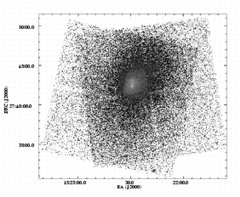
Figure 1.— Raw merged ACIS-I X-ray image of two observations in the 0.3–10 keV band, uncorrected for background or exposure. The image was binned by a factor of 5 in RA and DEC and it is displayed in logarithmic scale. The irregular outline is the result of the different fields-of-view of the two observations. The two cross-like faint regions are the chip gaps between the four CCDs which make up the ACIS-I detector in each of the two observations.

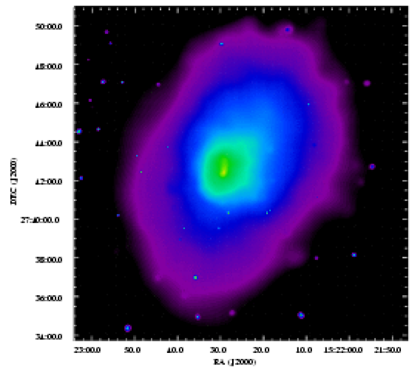
Figure 2.— Adaptively smoothed Chandra ACIS-I image of Abell 2065 in the energy band 0.3–10 keV, corrected for background and exposure. The image is displayed in logarithmic scale to emphasize low surface brightness emission. The faintest non-black regions have a surface brightness of $1.5\times 10^{-6}$ counts sec^-1 arcsec^-2.

Overall, the cluster emission is elongated from the northwest to the southeast. At the center, the image shows a compact, bright region. There is a more diffuse tail extending to the north at the center of the image. Although variations in the exposure confuse the region SE of the cluster center, there is evidence for a bow-shaped surface brightness discontinuity in this direction. There is also an extension in the emission further to the SE.

The optical DSS image of the cluster is presented in Figure 3a overlaid with the X-ray contours from the adaptively smoothed X-ray image (Fig. 2). The central cluster region is shown in Fig. 3b. The X-ray peak at the cluster center is displaced by 2$\farcs$4 from the position of the southern cD galaxy in the cluster.

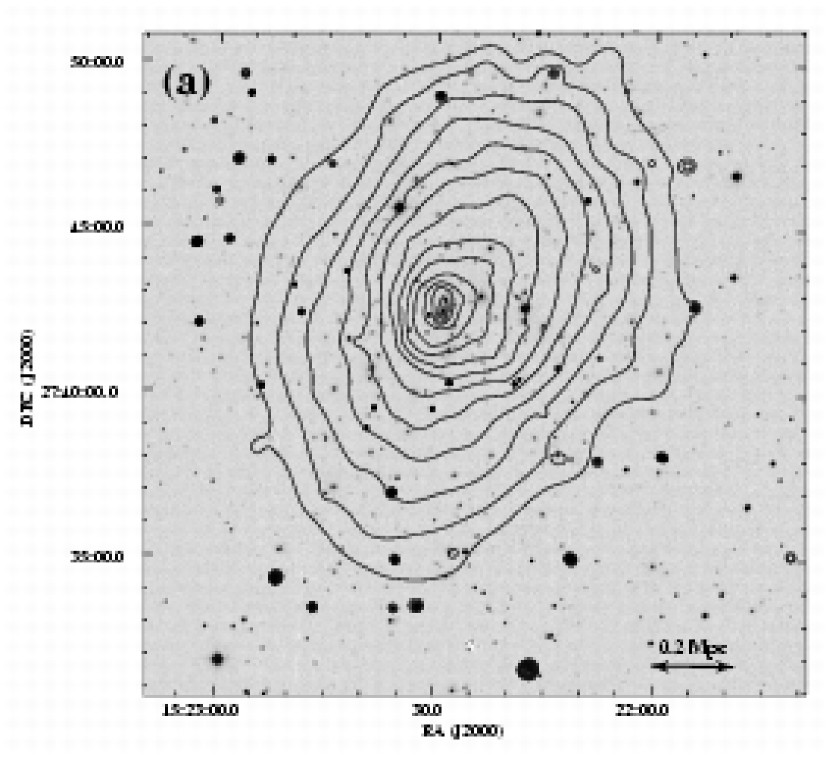
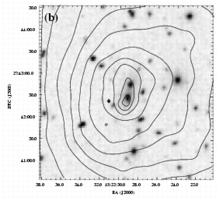
Figure 3.— Chandra X-ray contours overlaid on the Digitized Sky Survey image of Abell 2065. (a) 20$\farcm$5$\times$20$\farcm$5 field-of-view. The contours are spaced by a factor of $\sqrt{2}$ and they range from $1.5\times 10^{-6}$ to $1.4\times 10^{-4}$ counts sec^-1 arcsec^-2 for the diffuse gas. The brightest point sources reach surface brightness levels of $8.2\times 10^{-3}$ counts sec^-1 arcsec^-2. (b) The central 4′$\times$4′ cluster region. Note that only the southern cD seems to be associated with the X-ray surface brightness peak.

Following Fabian et al. (2003), we applied an unsharp masking technique to reveal the structure in our data. Figure 4 shows an image of the central $\sim 84\arcsec\times 84\arcsec$ region of Abell 2065 produced by this technique. A 0.3–10 keV exposure-corrected image was smoothed with two gaussian kernels of 1$\farcs$476 and 14$\farcs$76 (3 and 30 pixels on the ACIS-I detector), respectively; Fig. 4 displays the difference between the two smoothed images. This particular set of kernels was selected from a range of sets, as they yield the highest degree of structure in the image; smaller kernels tend to unresolve the largest scale structure, while larger ones tend to wash out the high-resolution features of the image. Accurate positions of the centers of the two cDs have been determined from the 2MASS catalogue and they are marked with crosses in Figure 4. The position of the southern cD is close to the brightest region of X-ray emission in the cluster. The brightest X-rays come from a point just south of the center of the southern cD, and there is an elongated extension of the X-ray emission running about 25″ further to the south. There is also a more diffuse tail of emission to the north of the southern cD extending about 45″. The northern cD galaxy is located along the western edge of this tail, but does not correspond to a surface brightness peak or any other interesting feature in the tail.

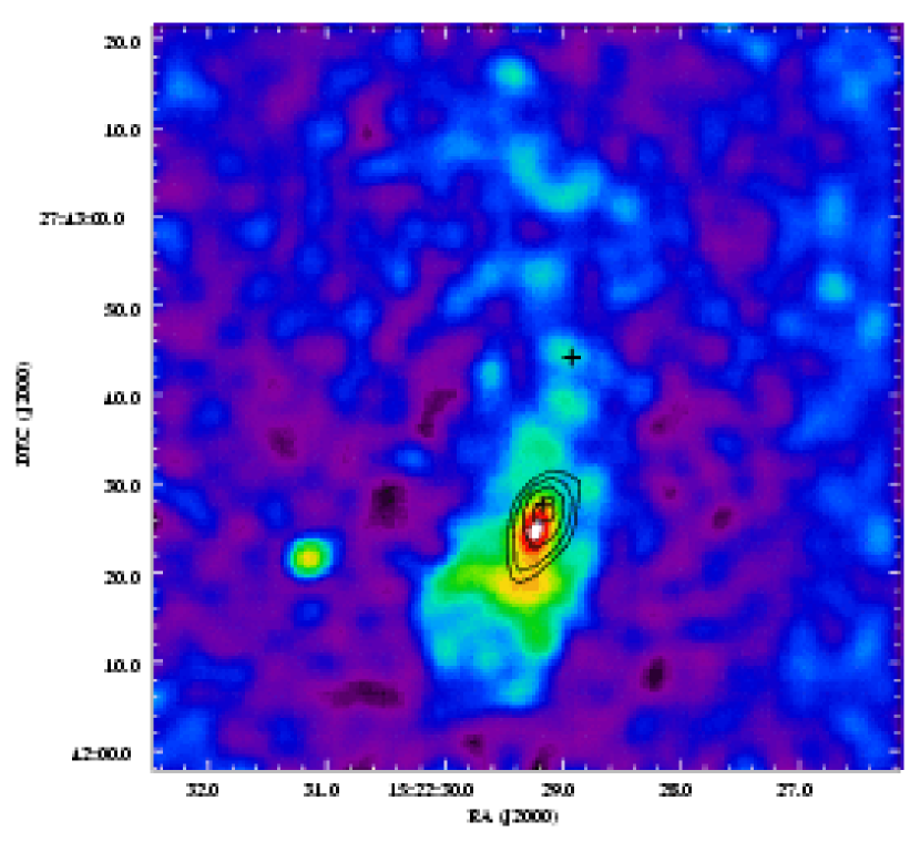
Figure 4.— Unsharp masked image of the central $\sim$ 84″$\times$84″ region of Abell 2065. The image was created by smoothing the 0.3–10 keV total (including the background) count rate image with two gaussian kernels, $\sigma=$ 1$\farcs$476 and $\sigma=$ 14$\farcs$76, and subtracting the first smoothed image from the second. The crosses indicate the positions of the centers of the two cD galaxies (2MASX J15222892+2742441 and 2MASS J15222917+2742275). The contours show the FIRST 1.4 GHz radio surface brightness. The lowest contour corresponds to a flux of 0.2 mJy per beam, and the contours are spaced by a factor of $\sqrt{2}$. The bright source to the E of the cluster center has no optical counterpart.

Based on much lower resolution ROSAT images, Markevitch et al. (1999) noted that the X-ray emission at the center of Abell 2065 was marginally resolved into two peaks; again, at the lower resolution of the ROSAT data, these were consistent with being located at the positions of the two cD galaxies. Markevitch et al. (1999) argued that the two peaks were two cool cores associated with separate subclusters with the two cDs at their centers, and that these two subclusters had merged. They suggested that the cool cores were still bound to the two cD galaxies, and drew conclusions about the central concentrations of the dark matter potentials of the two cDs. With our higher resolution Chandra data, the southern peak is indeed associated with the southern cD, but the northern peak appears to correspond to the more diffuse curved tail. This is not centered on the northern cD galaxy. Thus, only one of the cDs has retained a bound cool core, although the northern cD may not have had a cool core prior to the merger.

The morphology of the northern tail and its apparent connection with the southern cD suggests that the tail may be gas which has been stripped from this cD. Alternatively, it is possible that it was removed from the northern cD, which now retains very little hot gas.

The southern cD galaxy (2MASS J15222917+2742275) is also a faint radio source (3.09 mJy at 1.4 GHz). In Figure 4, the radio contours from the FIRST survey are superposed on the unsharp-masked X-ray image of the center of the cluster. The radio source is small and the core is not very well resolved in the FIRST data, although the extent to the south is much larger than the FIRST beam size. The peak in the radio surface brightness is nearly coincident with the center of the cD galaxy and the peak in the X-ray surface brightness. The radio source is extended to the SE of the center of the cD galaxy. The radio extension corresponds closely to a similar extension in the X-ray emission. If both are due to ram pressure as the southern cD moves relative to the surrounding intracluster gas, this would indicate that the galaxy is now moving to the NW. If this is the case, then the more extended tail to the north is due to gas removed from the northern cD. On the other hand, the radio/X-ray extension to the south might be due to buoyancy, or to more complex gas motions in the core of the cluster.

4. Spectral Analysis

We extracted spectra of selected regions in the Chandra image separately for the two datasets. Flux weighted ancillary files and response matrix files were calculated with the CIAO tools MKWARF and MKRMF. Because in CIAO 3.2 the tool MKRMF did not work properly with the latest calibration files (CALDB 3.0), the data were reduced anew using the previous calibration (CALDB 2.8); the blank sky background files were also processed to match the observations. The calibration included the temporal and spatial variation of the soft X-ray quantum efficiency degradation due to the build-up of material on the optical blocking filter. The data were screened using the same good time intervals of low background brightness as in § 2. The spectra for each dataset were independently grouped, so that each bin contained at least 25 counts. In both observations, the spectrum at energies below 0.7 keV is affected by sharp effective area and quantum efficiency variations, while at energies above 6.5 keV the background is dominant; thus we restrict our spectral extraction in this photon energy range 0.7–6.5 keV. The spectra from the two datasets were simultaneously fit in this range using the same spectral model. In most cases, the spectra were fit with the WABS model for the absorption and the APEC model (Smith et al., 2001) for the thermal emission. In most fits, the absorbing column density was held fixed to the Galactic value of $N_{H}=2.9\times 10^{20}$ cm^-2. The fitting was performed with XSPEC (Arnaud, 1996), version 11.3.

4.1. Global X-ray Spectrum

First, the spectrum was extracted for the largest elliptical region which roughly followed the shape of the X-ray isophotes and which fell completely within the fields-of-view of both observations; this was an elliptical region centered on the southern cD galaxy, with semimajor and semiminor axes of 6$\farcm$3 and 4$\farcm$9, respectively, aligned with the orientation of the cluster emission (PA of the major axis at $-20\arcdeg$). The background was determined from the blank sky background files discussed in § 2.

Table 1 summarizes the resulting spectral fits. A single temperature model with Galactic absorption provided a good fit to the spectrum, with a value of $\chi^{2}$ per degree-of-freedom, $\chi^{2}_{r}$, very close to unity. The observed spectrum and best-fit model are shown in Figure 5. We tested the effect of allowing the absorption column density to vary; this marginally improved the fit, and yielded a column density consistent within the errors with the Galactic value (here and elsewhere, the F-test has been used to compare the fits). Therefore, in the following, we keep the column density fixed at the Galactic value. The best fit model shows a residual structure at $\sim$ 2 keV; it is known that this is generally due to the rapid variation in Chandra’s effective area near the Ir edge of the telescope’s mirror. We refit the spectrum removing this region (1.8–2.3 keV). This improved the fit, but the model parameters were essentially identical to those including the Ir edge region.

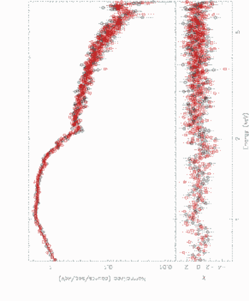
Figure 5.— Global X-ray spectrum of Abell 2065, with the best-fit single temperature APEC model attenuated by Galactic absorption. Circles (black) and squares (red) represent Obs. 1 and Obs. 2 spectra, respectively. [See electronic edition of the Journal for a color version of this figure.]

In § 4.2 below, we will see that the cluster contains gas with an extremely wide range of temperatures. Thus, it is somewhat surprising that the global cluster spectrum is well fit by a single temperature model, and so we tried a two temperature model. The fit was improved, but the second thermal component was essentially unconstrained, having a lower limit of about 10 keV. This indicates that the cluster contains some very hot gas, but the global spectrum is not very useful for characterizing this gas.

Previous ROSAT and ASCA images and spectra suggested that Abell 2065 contained a weak cooling flow (Markevitch et al., 1999, 1998; Peres et al., 1998; White, 2000). Thus, we also tried a model of a single temperature cluster thermal emission combined with a cooling flow component whose upper temperature was fixed at the cluster ambient temperature and whose lower temperature was 0.08 keV. The abundance in the cooling flow component was fixed to that of the ambient cluster gas. XSPEC’s MKCFLOW, which was used to model the cool core, utilizes the MEKAL atomic library (Liedahl et al., 1995) to calculate atomic line emission. In order to use consistent atomic data between the ambient thermal emission and the cool core model components, the MEKAL model was employed to model the cluster component. We first tested what effect the use of the MEKAL model had on the best-fit parameter values as determined with the APEC model. The fit was not significantly improved, and the cluster temperature and abundance were consistent within the errors with the values obtained with APEC.

Combining the thermal and cooling flow components did not produce a better fit to the spectrum, and the best-fit cluster temperature and abundance values were consistent with those derived from the MEKAL model alone. The cooling rate for the model was $\sim$ 4${}^{+11}_{-4}$ M_☉ yr^-1, which is in agreement with the measurement of Peres et al. (1998), but also consistent with no cooling.

The best-fit single temperature model is consistent with results from the ASCA spectrum. Markevitch et al. (1998) found a best-fit single temperature of $kT=5.4\pm 0.3$ keV; almost exactly the same result was derived by White (2000) and Ikebe et al. (2002). On the other hand, David et al. (1993) derived a temperature of $kT=8.4^{+3.3}_{-1.8}$ keV from the Einstein MPC detector. Both our temperature map (§ 4.2, below) and the previous temperature map from ASCA (Markevitch et al., 1999) show that the outer, southern parts of the cluster are very hot. Thus, the higher Einstein MPC average temperature probably results from the very large field of view and a very hard X-ray response of this instrument.

Table 1Models Fit to the Global X-ray Spectrum

			1st Component			2nd Component
Model	$\chi^{2}_{r}$	$N_{H}$	$kT$	Abundance		$kT$	Abundance	$\dot{M}$
(WABS *)		($10^{20}$ cm-2)	(keV)	(Solar Units)		(keV)	(Solar Units)	$M_{\sun}$ yr-1
APEC	852/731=1.166	$2.9$	$5.520\pm 0.143$	$0.309\pm 0.039$		$\cdots$	$\cdots$	$\cdots$
APEC	851/730=1.165	$2.366\pm 0.676$	$5.627^{+0.200}_{-0.198}$	$0.310^{+0.040}_{-0.039}$		$\cdots$	$\cdots$	$\cdots$
APEC — Ir region	725/661=1.097	$2.9$	$5.513^{+0.143}_{-0.141}$	$0.310\pm 0.039$		$\cdots$	$\cdots$	$\cdots$
APEC+APEC	817/728=1.122	$2.9$	$4.035^{+0.217}_{-0.288}$	$0.459^{+0.063}$		$11.547_{-1.869}$	$0$	$\cdots$
MEKAL	839/731=1.148	$2.9$	$5.541^{+0.125}_{-0.120}$	$0.282\pm 0.034$		$\cdots$	$\cdots$	$\cdots$
MEKAL+MKCFLOW	839/730=1.149	$2.9$	$5.609^{+0.238}_{-0.179}$	$0.282\pm 0.034$		$\cdots$	$0.282$	$4^{+11}_{-4}$

4.2. Temperature Maps

Since the Chandra X-ray image of Abell 2065 shows a wealth of structure and the previous ASCA temperature map showed evidence for a shock structure to the south, we have constructed maps of the projected temperature using the Interactive Spectral Interpretation System, ISIS (Houck et al., 2000). The temperature maps for two regions centered on the southern cD galaxy have been computed and are presented in Figure 6. Fig. 6a shows a region that stretches 10$\farcm$5 $\times$ 10$\farcm$5 across, while the central 4$\farcm$1 $\times$ 4$\farcm$1 of the cluster is presented in Fig. 6b.

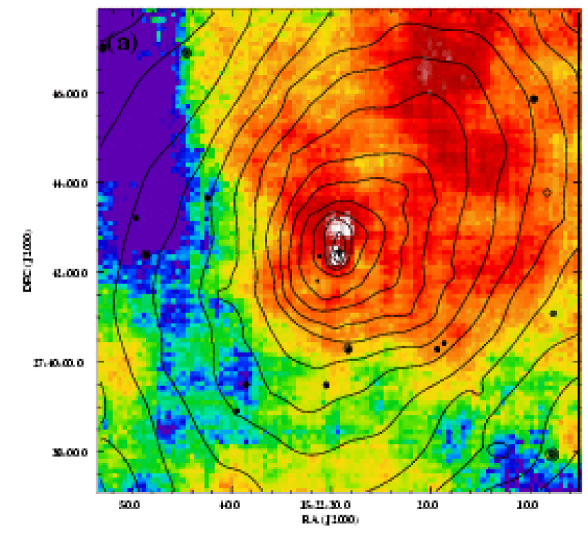
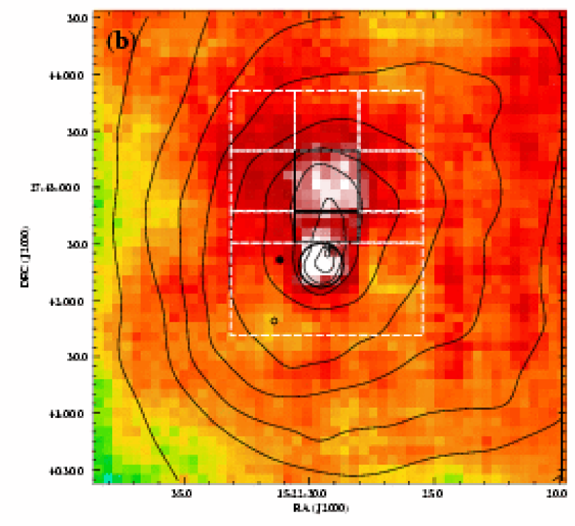
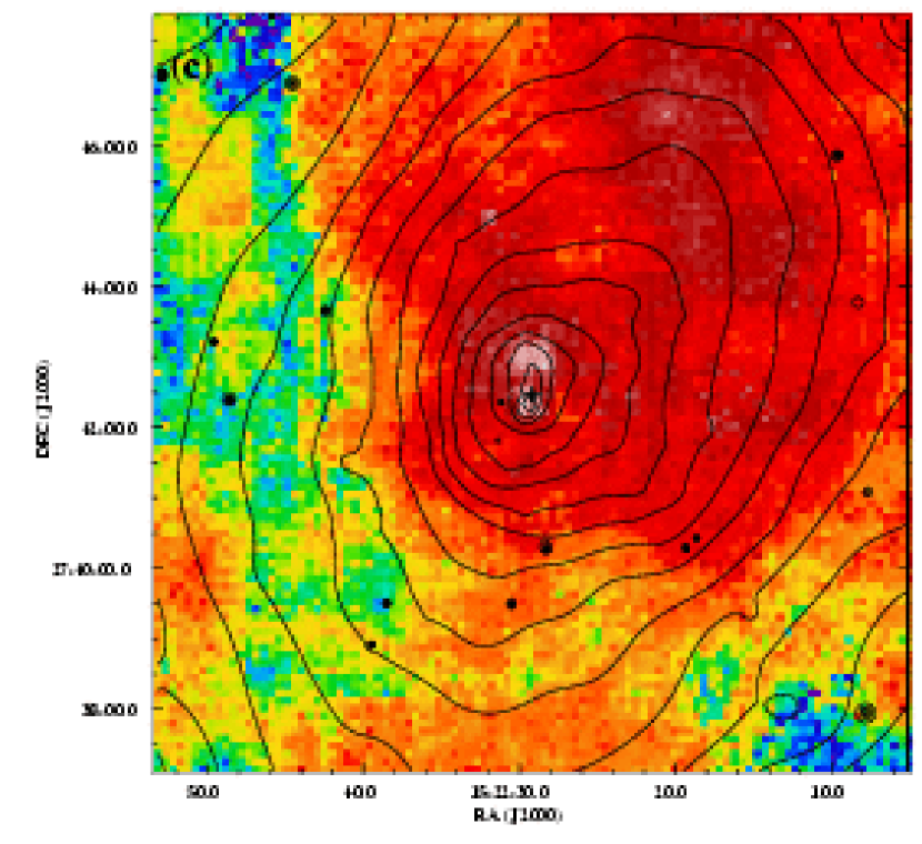
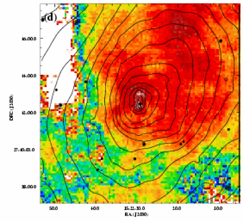
Figure 6.— Temperature maps derived from fitting the combined spectra from the two observations. The overlaid Chandra X-ray surface brightness contours are similar to those shown in Fig 3. The cross denotes the position of the southern cD galaxy. (a) Map of a 10$\farcm$5$\times$10$\farcm$5 field-of-view of the cluster. (b) Map of the central 4$\farcm$1$\times$4$\farcm$1 of the cluster. The geometrical shapes illustrate the areas used for the extraction of cluster spectra (solid lines) and for the local background to those spectra (dashed lines), as described in § 4.3. (c-d) Negative and positive, respectively, 90% error maps of the temperature map shown in a.

The temperature calculations were performed as follows. At each pixel position, the spectrum from each observation was extracted, requiring that at least 800 net counts be included in the energy range of 0.7–6.5 keV. The extraction region was a square box centered at the pixel center, whose size varied having a maximum value of 500 ACIS-I pixels for the larger scale map (Fig. 6a) and $\sim$ 300 ACIS-I pixels for the cluster center map (Fig. 6b). The box size was adaptively determined so that the number of observed counts in the particular region, over the entire energy spectrum, was between 1.5 and 2 times the nominal 800 counts, in order to account for background subtraction as well as for the fact that the fitting occurs over a limited energy range (0.7–6.5 keV). For each observation, the background was extracted from the blank sky background files, for the same energy band; for each pixel, the region that was used was the same as the one used with the source spectrum. The spectra were combined in ISIS, requiring at least 25 counts per bin, and subsequently fit with a thermal model with Galactic absorption. The abundance was held fixed at the value derived by fitting the global spectrum with a thermal model (Table 1, first row).

The temperature map of Figure 6a reveals several spatially separated regions of lower and higher projected temperatures. The lowest temperatures are found to the NW and in a limited region to the SE of the southern cD galaxy. The entire region NW of the center of the cluster is moderately cool. On the other hand, the hottest gas is at radii of $\lesssim$ 3′ SE of the southern cD. The typical temperature to the NW of the cluster center is $\sim$ 5 keV, while the hotter SE region has much higher temperatures of $\sim$ 10 keV. These values are in good agreement with the values Markevitch et al. (1999) derived from ASCA data (regions #2 and #4, respectively, in their paper). These hot and cool regions seem to be separated by a bow-shaped feature that runs from the NE to the SW of the cD, at $\sim$ 3′ from it. Especially to the SE of the cD, the temperature gradient is quite steep, increasing by 7 keV over scales smaller than an arcminute in some cases. The temperature structure of that region and the high temperatures encountered in it, in combination with the bow-shaped feature on the SE of the cD suggest the presence of a shock front beyond $\sim$ 3′ to the SE of the southern cD.

Figure 6c-d show, respectively, the negative and positive temperature error at each pixel position, as calculated for 90% error estimates. The average error in these images is 1.56 keV and 1.70 keV, respectively, for the negative and positive error images. It is obvious from these images, that the hot region to the NE of the southern cD (Fig. 6a) is associated with large errors, and thus it could be an artifact of poor statistics. Note that Markevitch et al. (1999) did not find high temperatures in this region (region #5) with ASCA.

At smaller scales near the cluster center (Fig. 6b), the temperature map reveals at least two interesting structures. The coolest gas in the map seems to be associated with the X-ray extension to the south of the southern cD galaxy, and slightly displaced from the center of this galaxy. This would be unusual for a cool core in a relaxed system; generally, they are very accurately coincident with the center of the central cD. As noted previously from Fig. 4, both the thermal X-ray and nonthermal radio plasma near the southern cD appear to be displaced to the south. The region just north of the southern cD seems to be warmer. However, the tail further to the north is cooler (the second coolest region in the cluster).

4.3. Cool Cluster Regions

Whether the northern tail is actually a distinct gas concentration from the southern extension is not clear from the error images (Fig. 6c-d). The warmer material that bridges these two regions has a projected temperature consistent with a monotonic radial increase from the southern extension to the northern tail, but also with a higher temperature than the surrounding regions.

In order to address the significance of the apparent temperature increase and to provide a more accurate assessment of the spectral properties of these regions, we have extracted spectra and fit them with a thermal APEC model with Galactic absorption. The geometric regions defined for the extraction purposes were such that they trace these features in the temperature maps (Fig. 6), the raw data image, as well as the unsharp-masked image (Fig. 4). These regions are displayed in Fig. 6b by the solid-line geometrical figures. In detail, the spectrum of the very cool southern extension was extracted from a 12″ radius circle centered 10$\farcs$1 south of the southern cD center. The spectrum of the warmer region between the two coolest cluster regions (hereafter, the ‘bridge’) was extracted from a rectangular region, $\sim$ 34″$\times$16″, elongated along the east-west direction and centered 11$\farcs$1 to the north of the southern cD. Finally, the spectral extraction for the northern tail was performed from a rectangular region centered 35$\farcs$7 to the north of the cD, which was $\sim$ 34″$\times$32″ in size and run in the east-west direction.

Since these regions are located at the center of the cluster, their spectra are heavily contaminated by foreground and background X-ray emitting ICM along the line-of-sight. Thus, accounting for the background has been accomplished in two different ways: by extracting a local background from the events files themselves and by using the blank sky background files. The former case has the advantage that foreground/background cluster emission is accounted for in a direct manner, and thus the derived spectral properties should refer to represent the emission of the small cool region near the cluster center. The dashed-line rectangles in Fig. 6b illustrate the regions used for the local background. In detail, the local background for the southern cool core was taken from a rectangular region, $\sim 102\arcsec\times 49\arcsec$, elongated in the east-west direction to avoid emission from the northern structure and centered $\sim$ 22″ south of the southern cD, excluding, of course, the circular region of the cool core and point sources. The local background for the bridge was extracted from regions identical to and adjacently positioned to the east and west of the rectangular region used with the spectrum extraction. For the tail, the background was extracted from 5 rectangular regions, identical and contiguous to the one used for the spectrum extraction; three of these regions were positioned to the north, and one each to the east and west of the extraction rectangle.

On the other hand, when we use the blank sky background spectrum we model the foreground and background emission by including a second thermal component whose temperature and abundance were fixed to the best-fit values from the global cluster X-ray spectrum. The normalization of this component was allowed to vary.

The best-fit models for the southern cD extension are shown in Table 2. The two techniques yielded consistent results. The blank-sky background yielded a better fit, although with higher uncertainty in the best-fit values. The abundances are essentially unconstrained with both techniques. To test if the use of the global cluster temperature is a good approximation for the mean ICM temperature along the line-of-sight, we fit the spectrum allowing the temperature and abundance of the cluster component to vary. The fit improved, but the line-of-sight thermal component is now unconstrained, while the uncertainty of the cool core temperature slightly increased. The abundances are again unconstrained.

Consistent results are obtained for the bridge spectrum, as shown in Table 2. The local background technique yields a better fit and a higher temperature. Using the global spectrum temperature to model the cluster emission did not improve the fit. This suggests that the global spectrum may not provide an adequate description of cluster emission along this line-of-sight. Thus, we allowed the second thermal component to vary but unfortunately the best-fit values for both thermal components were unconstrained. This, in combination with the uncertainty in the abundances in both techniques, is a consequence of the low number of counts in this region in both observations.

The two techniques yield consistent results for the northern tail, as shown in Table 2. The spectrum is adequately fit with either technique, though the blank-sky background technique yielded a better fit. Again, allowing the cluster component to vary slightly improved the fit, but the computed best-fit parameters are more uncertain. As suggested by the temperature map (Fig. 6), the northern tail is cooler than the global temperature. The metallicity is poorly constrained, but it appears to be higher than the cluster average value.

Overall, these results suggest that the blank-sky background technique provides slightly better fits, albeit with higher uncertainties. However, the temperature errors that either technique yields are large enough to prevent a definitive assessment of the significance of the temperature increase at the position of the bridge. In § 7.4.1 we argue that the northern tail is a trail of gas that has been stripped from the southern cD galaxy’s cooling core.

Table 2Spectral Fits for the Cluster’s Coolest Regions

			Local Spectrum			Cluster Emission
Region	Background	$\chi^{2}_{r}$	$kT$	Abundance		$kT$	Abundance
			(keV)	(Solar Units)		(keV)	(Solar Units)
South cD Extension	Local	63.594/71 = 0.896	$2.824^{+0.366}_{-0.322}$	$1.096^{+0.716}_{-0.483}$
South cD Extension	Blank Sky	58.765/70 = 0.839	$2.073^{+0.893}_{-0.411}$	$2.239^{+2.716}_{-1.016}$		5.519	0.308
South cD Extension	Blank Sky	58.281/68 = 0.857	$2.094^{+0.961}_{-0.508}$	$4.942_{-4.942}$		$5.148^{+9.137}_{-1.238}$	$0.101^{+0.891}_{-0.101}$
Bridge to Tail	Local	45.227/59 = 0.767	$3.873^{+1.255}_{-1.010}$	$1.591_{-1.242}$
Bridge to Tail	Blank Sky	53.381/58 = 0.920	$2.128^{+2.313}_{-0.528}$	$1.746_{-1.536}$		5.519	0.308
Northern Tail	Local	96.301/92 = 1.047	$3.374^{+0.714}_{-0.466}$	$0.916^{+1.293}_{-0.492}$
Northern Tail	Blank Sky	90.393/91 = 0.993	$2.324^{+1.591}_{-0.525}$	$1.946_{-0.478}$		5.519	0.308
Northern Tail	Blank Sky	89.128/89 = 1.001	$2.866^{+1.138}_{-0.758}$	$0.864_{-0.410}$		$8.871_{-4.054}$	$6.2_{-6.2}\times 10^{-6}$

5. X-ray Surface Brightness Profile

The temperature map (Fig. 6a) shows a complex structure with an inner hot region and an outer very hot region to the SE of the southern cD galaxy. In addition, there are steep surface brightness gradients in the same regions, displayed by the isophotes in Fig. 3; these two results suggest the presence of a cold front and a shock front in this region.

In order to better understand the gas physics in this cluster region, we have extracted the surface brightness profile from a pie circular aperture centered on the southern cD galaxy and lying to the SE. This pie region stretches between 100° and 180° in PA and out to $\sim$ 10′ from the center of the cD in radius; a total of 45 annuli were used, their radial extent varying from $\sim$ 3″, for the innermost, to $\sim$ 30″, for the outermost. The background was taken from the merged blank sky background file (§ 2). The resultant surface brightness distribution is presented in Fig. 7a.

Figure 7.— (a) Detailed surface brightness profile of the region SE of the southern cD galaxy. The rapidly declining inner portion of the plot (cluster’s cool core) is succeeded by a possibly shocked region. The outer part of the profile is adequately fit with a $\beta$-model. (b) Local electron density distribution. Notice the clear presence of discontinuities at $\sim$30″ and $\sim$100″. The discontinuity at $\sim$200″ is artificial, as it reflects the moderate statistics obtained for that region, in which the chips gaps of the two observations overlap.

The profile generally shows a rather smooth decline with radius. Superposed on that, we find two interesting features. First, there is a sharp decline over the inner part of the profile, terminated by a discontinuity at $\sim$ 30″ from the center. This discontinuity is associated with the cool southern cD extension. This indicates that this feature is bounded by a cold front at its southern edge. Additionally, a region of excess X-ray emission, with respect to the outer part of the brightness profile (see below), is found to stretch from $\sim$ 30″ out to $\sim$ 100″. This is followed by a discontinuity, where the surface brightness drops by a factor of $\sim$ 1.7 over a radial extent of 10″, reminiscent of surface brightness jumps observed across shocks, as well as cold fronts. Notice that this discontinuity is not associated with the shock-like features seen in Fig. 6a. On the contrary, the outer 500″ of the profile are consistent with a $\beta$-model surface brightness distribution ($\beta=0.63$ and $r_{core}=$ 218″ or 292 kpc), lacking evident shock signatures.

We have attempted to fit a cold front surface brightness model to the inner part of the profile, but the excess X-ray emission region that extends immediately outwards complicates the analysis. Instead, in an attempt to better study the gas behavior across the entire profile, as well as understand the nature of the features seen in Fig. 7a, we have deprojected the surface brightness profile. The assumptions that underlie this method are those of spherical symmetry with respect to the gravitational potential peak, identified in our case with the southern cD galaxy, and of uniform electron density distribution within each shell. The electron densities are presented in Figure 7b.

The local density distribution clearly demonstrates the two features seen in the projected profile of Fig. 7a. There is rather rapid central decline until $\sim$ 30″, where a discontinuity occurs. The average density just inside the cold front region is $\overline{n}=2.67^{+0.59}_{-1.09}\times 10^{-2}$ cm^-3. Then the density undergoes a shallow decline: it drops by a factor of 1.2 over a radial interval of $\sim$60″. A dramatic density jump of $\sim$2 is observed at $\sim$ 100″, followed by a steeper decline. Again, this jump is consistent with being either a shock or a cold front. The nature of this discontinuity is examined in § 7.1. Finally, there seems to be another discontinuity at $\sim$ 3′ from the southern cD, which coincides with the position of the bow-shaped feature of Fig. 6a. However, this jump also coincides with the region in our merged raw data where the chip gaps of the two observations overlap. The magnitude of the density errors at the position of this jump relative to the errors of adjacent values, in combination with the absence of any strong deviations from the smooth isothermal decline in the surface brightness profile (Fig. 7a), indicate that the jump is probably an artifact of low number statistics at the position of the chip gaps.

6. Spectral Deprojection

Our interpretation of a shock propagating through the cluster ICM has been stimulated by the temperature map structure (Fig. 6a). However, the temperature map does not reflect the local gas temperature (i.e. the gas at a specific distance from the cluster center), rather the average temperature of the X-ray emitting gas along the line-of-sight. For instance, if a shock is indeed propagating beyond $\sim$ 3′ SE of the southern cD, the projected temperatures of the central cluster region, as shown in the temperature map (Fig. 6b), are overestimates of the true local temperatures.

In order to disentangle local from projected emission, and gain deeper insight on the gas physics of this region, we have deprojected the spectra of a set of regions. Specifically, we have defined a set of 8 regions stretching from the center of the optical cD out to a radius of $\sim$ 6$\farcm$4 and covering the same PA interval as the regions used with the surface brightness deprojection algorithm, namely from 100° to 180°. These regions have been selected to fall on the ACIS-I detector in both observations, and in particular to trace features of the raw data image primarily, as well as of the temperature map. For instance, the innermost region covers most of the area used to examine the spectral properties of the southern cD extension, discussed in § 4.3, while the third annulus from the center traces the 100″ brightness discontinuity. They are displayed in Figure 8. In these regions, the total net counts from both observations range between 1600 and 4200.

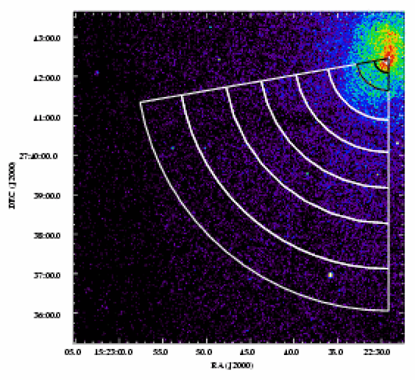
Figure 8.— Raw photon image in the range 0.7–6.5 keV of the $\sim$ 8$\farcm$4$\times$8$\farcm$4 region SE of the southern cD. The image has been smoothed with a boxcar kernel $\sim$ 1″ and displayed in histogram equalization scale. The annuli show the regions used for the deprojection. The common vertex coincides with the center of the southern cD. The same overall region was used with the surface brightness profile deprojection.

The spectra of these regions were extracted from each observation, as described in § 4. For each region, the flux weighted sum of the spectra from the two observations for both the source and the background were calculated, and a flux weighted average detector response was produced. The subsequent fitting was performed in the energy band 0.7–6.5 keV, grouping bins to contain at least 25 counts, as needed.

The deprojection was carried out with XSPEC in two different ways; in both, the shells’ local emission was modeled with a thermal model with Galactic absorption. First, XSPEC’s mixing model projct was used. projct calculates the projection matrix of each of the overlying shells on the area of each annulus and computes the total projected emission on that annulus. The fitting occurs simultaneously for all annuli and upon completion the emission integral of the entire spherical shell is returned, along with the best-fitting temperature and abundance values.

Fitting all the spectra simultaneously has the effect that the best-fit values of the outer annuli are affected by those of the inner annuli. To reduce the effects of this feature of the algorithm, we have fit the individual spectrum of the outermost annulus with an APEC thermal model with Galactic absorption. Then, we used the obtained temperature and abundance values to fix the spectral parameters of the outermost shell during the deprojection and allowing all others to vary we obtained a best-fit $\chi^{2}_{r}$ value of 0.96. The abundance was rather poorly constrained.

An alternate approach was also followed. In this, the spectral fitting occurred successively for the different shells. Starting with the outermost spectrum, the best-fit values of the spectral parameters were determined. Subsequently, the spectrum of the inner shell was fit with two thermal components, one of which was fixed to the best-fit values of the overlying shell, while the relevant normalization was adjusted to account for projection effects of the outer shell on the inner region and for different exposures between the two regions. This was done for the spectra of all interior regions, introducing thermal components to account for overlying emission, as needed. The abundance profile, again, was poorly constrained.

Comparing the two methods, it seems that, at least with our data, the latter method yields temperature values with smaller errors. The profiles presented in the following are based on these results.

6.1. Projected Temperature Profile

To check the consistency with the temperature map findings, we have produced the projected temperature profile for these regions, shown in Figure 9. The cool gas at the center of the cluster is followed by constant temperature gas out to a distance of $\sim$ 2$\farcm$5 from the cD. The temperature then rises by about 3 keV and maintains a constant value within the errors for $\sim$ 2′. This rise, also seen in the temperature map, has motivated the notion of shock propagation at that region. Subsequently, it drops to values consistent with those derived from ASCA data by Markevitch et al. (1999). The temperature map does not show a similar trend at that distance, but this is probably due to poor statistics at the map edge.

Figure 9.— Projected temperature profile in the PA interval 100°-180° SE of the southern cD galaxy.

Although the temperature rise and drop across 4′ is reminiscent of shock heating, the shock hypothesis is not supported by the detailed X-ray brightness profile (Fig. 7). In the contrary, as was mentioned in § 5, the outer 500″ are adequately fit with an isothermal model, and bear no strong evidence for compression. This hot, high entropy gas is then most likely a transient merger-induced effect. It apparently has a higher pressure than its surroundings and it is expected to dissipate in a few hundred Myr (a few sound crossing times).

6.2. Deprojected Temperature Profile

The deprojected temperature profile is presented in Figure 10a. The temperature in the central region is quite low, as already indicated in Table 2. The two high temperature points with very large errors around 3′ raise a concern. If the temperature in these regions has been overestimated, then deprojection might cause the temperatures of inner points to be underestimated; too much hot projected emission would have been subtracted from these points. In particular, the apparent temperature drop at about 2′ might then be an artifact of the overestimated temperature in the shells just outside. In any case, the drop at the position of the brightness discontinuity (at $\sim$1$\farcm$6) is not significant within the errors.

Given the highly uncertain temperature profile values, we have decided to use the average value of 5.5 keV to describe the gas temperature at the SE of the brightness discontinuity. This value is consistent with temperature of the two outer bins in the profile, and it is also consistent with the the pre-shocked region temperature as estimated from ASCA data (Markevitch et al., 1999). For error propagation purposes we adopt the values obtained by Markevitch et al. (1999) (region # 6 of Fig. 3c, therein), that is, $kT=5.5^{+2.5}_{-1.5}$ keV.

Figure 10.— Deprojected (a) temperature, (b) density, (c) pressure and (d) specific entropy profiles derived for the regions of Fig. 8. Note that the quantity plotted in the entropy profile is the residual of the regions’ entropy with respect to the average cluster entropy (see text for more details).

6.3. Density Profile

The definition for the thermal model normalization is that: $K=\frac{10^{-14}}{4\pi D^{2}_{A}(1+z)^{2}}\int n_{e}n_{p}dV$, where z the redshift to the cluster, $D_{A}$ is the angular diameter distance at that redshift, $n_{e}$ and $n_{p}$ the electron and proton number densities, respectively, and the integration is performed over the shell’s projected volume. Assuming uniform density distribution across each shell, and that $n_{e}/n_{p}=1.21$, this equation may be inverted to solve for the electron density. The quality of our data was sufficient to allow calculating accurate errors on the normalization values. We present the density profile in Figure 10b.

The profile shows structure similar to the one revealed by the higher resolution density distribution of Fig. 7b. The density in the central 30″ shell is high, and there is an abrupt density drop of about a factor of $\sim$ 4 outside of this region. The average density in the central 30″ is consistent with the average density derived from the detailed density profile (Fig. 7b). Another discontinuity is seen at $\sim$ 1$\farcm$6, coincident with the position of the brightness discontinuity. A monotonic decline beyond this point is interrupted by an increase at the outmost shell, where the higher value is an artifact of the assumption inherent to the deprojection algorithm of no external emission.

6.4. Pressure and Entropy Profiles

From the temperature and density profiles and assuming the ideal gas equation of state, we have calculated the radial profiles of gas pressure and specific entropy. They are presented in Fig. 10c–d, respectively. The entropy was computed using the equation $S=\frac{3k}{2}\ln{\frac{T}{n^{2/3}}}$. Note that the quantity plotted in the entropy profile is the residual of the average cluster entropy from the regions’ entropy, $\Delta S=S-S_{0}$. The global cluster entropy was calculated from the temperature value of the best-fit model to the global spectrum, and the average cluster density.

Note that the cool dense region at the center of the cluster seems to be in pressure equilibrium with its surroundings, while its entropy is the lowest in the cluster. This suggests that the core is convectively stable. The continuous pressure but greatly reduced entropy supports the notion that the southern X-ray extension of the southern cD is bounded by a contact discontinuity (a cold front).

The pressure shows a significant drop at $\sim$ 1$\farcm$6, which corresponds to the shock feature in Fig. 7a. There is no entropy decline between the same regions, as would be expected for a shock, although the errors are large.

The outer 2′ of the pressure profile are dominated by large errors, but they overall seem to follow a declining trend. Similarly, the outer portion of the entropy profile shows rather elevated values, as expected from the projected temperature profile (§ 6.1).

7. Discussion

7.1. Brightness Discontinuity at 100″

The detailed electron density profile (Fig. 7b) shows a clear discontinuity at $\sim$ 100″ ($\sim$ 140 kpc) to the SE of the southern cD. This discontinuity could be attributed to either a shock front or a cold front at that position. The critical parameter that would allow one to distinguish between these two possibilities is the value of the temperature contrast across the discontinuity. The ratio of the temperature for material ahead of the front to the temperature for material behind the front is expected to be greater than unity for a cold front and less than unity for a shock front. The projected temperature profile bears no evidence for any jump at that location, though the errors are significant. On the other hand, the deprojected temperature profile (Fig. 10a) shows a jump consistent with being greater than unity, but, as indicated earlier, it may be an artifact of the deprojection. Lacking strong evidence in either direction, we shall examine the implications of both scenarios on the kinematics of the merging system.

First, considering the shock possibility, the density compression across the discontinuity ($\rho_{2}/\rho_{1}=1.918^{+0.297}_{-0.384}$) can be used to constrain the kinematics of the merger. In principle, the Mach number ${\cal M}$ of a shock can be determined by employing the Rankine-Hugoniot shock equations (Landau & Lifshitz (1959), §85) for density or temperature jumps:

$$\frac{\rho_{2}}{\rho_{1}}=\frac{(1+\gamma){\cal M}^{2}}{2+(\gamma-1){\cal M}^{2}};\;\frac{T_{2}}{T_{1}}=\frac{(2\gamma{\cal M}^{2}-\gamma+1){\cal M}}{\gamma+1}\frac{\rho_{1}}{\rho_{2}}$$ (1)

where the subscript 2 denotes material behind the shock (the “post-shock” region), while subscript 1 refers to material ahead of the shock (the “pre-shock” region). For intracluster gas, $\gamma=5/3$. Using the above compression value with the first part of equation (1), we confirm the presence of a mildly supersonic outflow in this region ($\sim$ 30″-100″) with a Mach number of ${\cal M}=1.66^{+0.24}_{-0.32}$ at the position of the shock. The observed temperature jump is much smaller than the theoretical value, $T_{2}/T_{1}=2.78^{+0.88}_{-1.13}$, although consistent within the errors. Similarly, the observed and the theoretical values of the pressure ratio are consistent within the errors, although the pressure is not independent of either the density or the temperature.

On the other hand, if the discontinuity is due to a cold front, the velocity can be derived based on the stagnation condition at the cold front (Vikhlinin et al., 2001), which gives the ratio of the pressure at the stagnation point at the cold front ($P_{\rm st}$) to that far upstream ($P_{1}$):

$$\frac{P_{\rm st}}{P_{1}}=\left\{\begin{array}[]{cl}\left(1+\frac{\gamma-1}{2}{\cal M}^{2}\right)^{\frac{\gamma}{\gamma-1}}\,,&{\cal M}\leq 1\,,\\ {\cal M}^{2}\,\left(\frac{\gamma+1}{2}\right)^{\frac{\gamma+1}{\gamma-1}}\,\left(\gamma-\frac{\gamma-1}{2{\cal M}^{2}}\,\right)^{-\frac{1}{\gamma-1}}\,,&{\cal M}>1\,.\\ \end{array}\right.$$ (2)

Here, ${\cal M}$ is the Mach number of the cold front relative to the upstream gas, and $\gamma=5/3$. We use the density at $\sim$ 90″ (Fig. 7) and the temperature at 1$\farcm$2 (Fig. 10a) to approximate the pressure at the stagnation point. We have chosen to approximate the pressure far upstream with the density value at $\sim$ 4′ from the cD and the average temperature 5.5 keV (§ 6.2). Then, the pressure contrast is $\sim$ 5, which implies that the cold front is moving through the hotter gas with a Mach number of ${\cal M}=1.93^{+0.24}_{-0.19}$. This should be viewed as an upper limit to the cold front velocity, as applying equation (2) for regions closer to the cold front suggests that the motion is still supersonic, but with smaller Mach numbers.

It is important to realize that, regardless the ambiguity of the nature of the discontinuity, these two scenarios bear consistent kinematical implications. In the following, we adopt the Mach number derived with the shock condition for the motion of the material at 100″.

The sound velocity for a perfect gas, under adiabatic conditions, is $c_{s}=\sqrt{\gamma k_{B}T/\mu m_{p}}$. Taking the mean molecular weight of the ICM to be $\mu=0.6$, and using the average temperature 5.5 keV, the far upstream sound speed is $\sim$ 1200 km s^-1. Then, the velocity of the shock or cold front is $v={\cal M}c_{s}$, or $\sim$ 2000 km s^-1, similar to the value derived by Markevitch et al. (1999).

7.2. Stagnation Condition at the Cold Front

The cool core surrounding the southern cD appears to be bounded on its southern edge by a cold front. An estimate of the merger relative velocity can also be derived based on the stagnation condition at the cold front, equation (2). In this case, ${\cal M}$ is the Mach number of the cool core relative to the upstream gas, and $\gamma=5/3$. As in the cold front scenario in § 7.1, the far upstream pressure has been approximated using the density at a distance of $\sim$ 4′ SE of the southern cD and the average temperature of 5.5 keV. The stagnation point should be in pressure equilibrium with the material inside the cool core; the density immediately interior to the front ($r\approx$ 29″, Fig. 7b) and the deprojected core temperature can be used to approximate the stagnation pressure. For this set of regions, the pressure ratio is about 4, and the Mach number is ${\cal M}=1.74^{+0.22}_{-0.18}$. This value agrees with the Mach number of the discontinuity at 100″. Especially in the case that the latter is indeed a cold front, the discrepancy between the Mach number values of the two structures could be understood as being due to acceleration gained by the exterior front, as it propagates down a density gradient.

7.3. Survival of the Cool Core

The cool, low entropy, southern extension has been identified with the cooling flow core of the southern cD. The condition for survival of the cool core is (roughly) that the ram pressure force of the incident ambient gas be less than the gravitational restoring force of the potential of the cluster core on the cooling core gas. Assuming that the cooling core was initially in hydrostatic equilibrium, the condition for the survival of the cool core is (Fabian & Daines, 1991; Markevitch et al., 1999; Gómez et al., 2002):

$$\rho_{\rm sc}v_{\rm rel}^{2}\lesssim P_{\rm cc}-P_{\rm am}\,,$$ (3)

where $\rho_{\rm sc}$ is the cool core density of the infalling cluster, $v_{\rm rel}$ is the relative velocity, $P_{\rm cc}$ is the pressure at the center of the cool core, and $P_{\rm am}\ll P_{\rm cc}$ is the ambient pressure of the main cluster around the cool core. One concern is that this condition assumes that the cooling core gas is bound to the dark matter potential of the main cluster; in Abell 2065, the center of the cool core is displaced by $\sim$ 12″ or 16 kpc from the center of the cD. However, the fact that the cool core remains fairly intact probably implies that this condition is not strongly violated.

The local density at 12″ SE of the southern cD (Fig. 7b) has been employed for the value of $\rho_{cc}$; the central cooling core pressure $P_{\rm cc}$ was estimated utilizing the deprojected core temperature. The ambient pressure $P_{\rm am}$ has been estimated from the density at 4′ SE of the cD, and the average temperature of 5.5 keV; it is negligible compared to $P_{\rm cc}$ and is ignored in the following. The choice for the infalling cluster initial central density is more difficult to make. Despite the ambiguity in the nature of the 100″ discontinuity and of the high temperature region between 2′ and 4′  the density immediately outside the 100″ front has been taken as a good approximation to $\rho_{\rm cc}$. Indeed, even with this uncertainty, equation (3) yields an upper limit to the relative subcluster velocity of $v_{\rm rel}\lesssim$ 1900 km s^-1, in accordance with the velocity derived from the kinematics of the 100″ discontinuity.

7.4. Dynamical Scenarios

The results that have been presented above can be compiled into a possible dynamical scenario concerning the history and the stage of the merger. In the following, we shall assume that the two cDs are located at the centers of the two merging subclusters, and that they are physically interacting with each other, (that is, their close proximity is not a projection effect). We will refer to the cluster centered on the southern cD as the southern cluster, and to the one centered on the northern cD as the northern cluster.

7.4.1 Unequal Mass Merger

We argue that the southern cluster is more massive than its northern counterpart; this is corroborated by the evidence presented above and by numerical simulations, as it will be shown below in detail. In this scenario, the northern cluster is falling into the more massive southern cluster. With the data, we can place an upper limit on the density contrast of the two subcluster cores by assuming that the gas ahead of the discontinuity at 100″ serves as an undisturbed sample of the initial northern cluster core conditions. We have considered the density at the position of the X-ray peak (at $\sim$ 2″, Fig. 7b) to be representative of the initial central density of the southern cool core. Then, the original density contrast has an upper limit of 27.

The absence of gas associated with the northern cD suggests that either the northern cool core has been disrupted during the merger or that the cluster did not possess a cool core originally. Although most subclusters have been observed to possess cool cores, the latter possibility cannot be dismissed.

The existence of the cold front at 30″ and the discontinuity at 100″ to the SE of the merger indicate that the southern cD is moving in this direction, having already experienced core crossing. Being the more massive and more dense part of the merger, the southern cluster has swept away most of the northern halo. The shock that was triggered during the early merger stages has displaced the northern cluster gas halo from the cluster’s center of mass and it is now projected to the SE of the merger, beyond the discontinuity at 100″.

The temperature map structure (Fig. 6a) is similar to the structure revealed in the temperature map of the 1:16 unequal mass merger, with a density contrast of 50, in the numerical simulations of Gómez et al. (2002), when viewed 250 Myr after core crossing. This indicates that the density contrast may be higher than the upper limit we determined above and that the time since core crossing is probably a few hundred Myr. This also suggests that the cluster has undergone core crossing probably for the first time.

In this scenario, the cool core displacement in the direction of motion can be understood in terms of the findings of Heinz et al. (2003). As the northern cluster was falling into the southern cluster from the SE (before core crossing), a shock wave was induced in the southern cluster. The shock may have reached the dense, cool core of the southern cluster, subjecting the latter to ram pressure stripping, which removed material originally located at the outskirts of the core. The generated pressure imbalance caused gas motions inside the cool core that resulted in gas transportation against the shock flow towards the contact discontinuity.

Finally, in the same scenario, the tail of cool gas that extends from the southern cD to the north can be understood as the material of the core outskirts that was removed by the incoming shock wave. Apparently, this gas did not meet the survival criteria set by equation (3), and it has been stripped from the cD. The small temperature difference between the cool core and the cold tail and their similar abundances (Table 2) suggest that this may indeed be the case, since the shock could displace as well as heat the gas to the observed values.

7.4.2 An Alternate Possibility

In § 3 the possibility was raised that the southern cD galaxy may be moving to the NW, and that the observed X-ray and radio extensions to the SE may be due to ram pressure stripping. In such a scenario, the two subclusters have not yet achieved closest approach and it is possible that they may be merging for the first time. However, there are certain issues this possibility fails to address. The discontinuity to the SE of the southern cD galaxy could be a manifestation of a shock wave, generated by the northern cluster as it falls through the ICM of the southern cluster. The induced ram pressure could be responsible for the displacement of the southern cluster cooling flow from the cD. These considerations in combination with the fact that no prominent shock front appears to the NW in our data, which would be generated by the southern cluster as it free-falls in the potential of its northern counterpart, suggest that the northern cluster must be more massive than the southern. Hence, it is remarkable that the cool core of the northern subcluster does not manifest itself as a region of enhanced X-ray emission in the X-ray brightness map of Fig. 2. Additionally, it is much harder to explain the nature of the cool tail that extends to the north of the southern cD, since the numerical experiments of Heinz et al. (2003) suggest that a shock front driven into a cooling flow would displace the latter in the incoming shock’s direction, but it would not distort its geometry to form an elongated leading structure. The possibility that this gas may have been expelled from the northern cD is not favored by the temperature consistency between the gas along the tail and the gas of the southern extension.

8. Summary

We have presented the results of a Chandra observation of the merging cluster of galaxies Abell 2065, which include the temperature maps of the central 10 arcmin² of the cluster emission and the spectral properties of the cooling flow of the southern cluster as well as a plume of cold gas emerging from the cD to the north. Evidence of shocks appear in the temperature maps to the SE of the merger and the deprojected density distribution of that region indicates the presence of a supersonic flow to the SE, with ${\cal M}\approx$ 1.7. However, the temperature data are not of sufficient accuracy to allow distinguishing between the shock wave and the cold front interpretation of this discontinuity. The cooling flow is displaced to the SE of the cD. At its southern edge, the cooling core appears to be bounded by a cold front.

Putting all these together, we propose that Abell 2065 is an unequal mass merger. The northern cluster seems to have fallen in the more massive southern cluster from the SE probably for the first time and having lost its gas content it is now moving to the NW, where it is now seen.

References

- Abell et al. (1989) Abell, G. O., Corwin, H. G., & Olowin, R. P. 1989, ApJS, 70, 1
- Abramopoulos & Ku (1983) Abramopoulos, F., & Ku, W. H.-M. 1983, ApJ, 271, 446
- Arnaud (1996) Arnaud, K. A. 1996, in ASP Conference Proceedings, Astronomical Data Analysis Software and Systems V, ed. Jacoby G. and Barnes J., (San Francisco: ASP), 17
- David et al. (1994) David, L. P., Jones, C., Forman, W., & Daines, S. 1994, ApJ, 428, 544
- David et al. (1993) David, L. P., Slyz, A., Jones, C., Forman, W., Vrtilek, S. D., & Arnaud, K. A. 1993, ApJ, 412, 479
- Fabian & Daines (1991) Fabian, A. C., & Daines, S. J. 1991, MNRAS, 252, 17P
- Fabian et al. (2003) Fabian, A. C., Sanders, J. S., Allen, S. W., Crawford, C. S., Iwasawa, K., Johnstone, R. M., Schmidt, R. W., & Taylor, G. B. 2003, MNRAS, 344, L43
- Fujita et al. (2004) Fujita, Y., Suzuki, T. K., & Wada, K. 2004, ApJ, 600, 650
- Gómez et al. (2002) Gómez, P. L., Loken, C., Roettiger, K., & Burns, O. 2002, ApJ, 569, 122
- Heinz et al. (2003) Heinz, S., Churazov, E., Forman, W., Jones, C., & Briel, U. G. 2003, MNRAS, 346, 13
- Houck et al. (2000) Houck, J. C., Denicola, L. A. 2000, in ASP Conference Proceedings, Astronomical Data Analysis Software and Systems IX, ed. Nadine Manset, Christian Veillet, & Dennis Crabtree, (San Francisco: ASP), 591
- Ikebe et al. (2002) Ikebe, Y., Reiprich, T. H., Böhringer, H., Tanaka, Y., & Kitayama, T. 2002, A&A, 383, 773
- Landau & Lifshitz (1959) Landau, L., D., & Lifshitz, E. M. 1959, Fluid Dynamics, (Reading, Massachusetts: Addison-Wesley)
- Liedahl et al. (1995) Liedahl, D. A., Osterheld, A. L., & Goldstein, W. H. 1995, ApJL, 438, 115
- Markevitch et al. (1998) Markevitch, M., Forman, W. R., Sarazin, C. L., & Vikhlinin, A. 1998, ApJ, 503, 77
- Markevitch et al. (1999) Markevitch, M., Sarazin, C. L., & Vikhlinin, A. 1999, ApJ, 521, 526
- Peres et al. (1998) Peres, C. B., Fabian, A. C., Edge, A. C., Allen, S. W., Johnstone, R. M., & White, D. A. 1998, MNRAS, 298, 416
- Postman et al. (1988) Postman M., Geller, M. J. & Huchra, J. P. 1988, AJ, 95 267
- Ricker & Sarazin (2001) Ricker, P. M., & Sarazin, C. L. 2001, ApJ, 561, 621
- Smith et al. (2001) Smith, R. K., Brickhouse, N. S., Liedahl, D. A., & Raymond, J. C. 2001, ApJ, 556, 91
- Vikhlinin et al. (2001) Vikhlinin, A., Markevitch, M., & Murray, S. S. 2001, ApJ, 551, 160
- White (2000) White, D. A. 2000, MNRAS, 312, 663