Axisymmetric simulations of magnetorotational core collapse: Approximate inclusion of general relativistic effects

We continue our investigations of the magnetorotational collapse of stellar cores by discussing simulations performed with a modified Newtonian gravitational potential that mimics general relativistic effects. The approximate TOV gravitational potential used in our simulations captures several basic features of fully relativistic simulations quite well. In particular, it is able to correctly reproduce the behavior of models that show a qualitative change both of the dynamics and the gravitational wave signal when switching from Newtonian to fully relativistic simulations. For models where the dynamics and gravitational wave signals are already captured qualitatively correctly by a Newtonian potential, the results of the Newtonian and the approximate TOV models differ quantitatively. The collapse proceeds to higher densities with the approximate TOV potential, allowing for a more efficient amplification of the magnetic field by differential rotation. The strength of the saturation fields ($\sim 10^{15}\ \mathrm{G}$ at the surface of the inner core) is a factor of two to three higher than in Newtonian gravity. Due to the more efficient field amplification, the influence of magnetic fields is considerably more pronounced than in the Newtonian case for some of the models. As in the Newtonian case, sufficiently strong magnetic fields slow down the core’s rotation and trigger a secular contraction phase to higher densities. More clearly than in Newtonian models, the collapsed cores of these models exhibit two different kinds of shock generation. Due to magnetic braking, a first shock wave created during the initial centrifugal bounce at subnuclear densities does not suffice for ejecting any mass, and the temporarily stabilized core continues to collapse to supranuclear densities. Another stronger shock wave is generated during the second bounce as the core exceeds nuclear matter density. The gravitational wave signal of these models does not fit into the standard classification. Therefore, in the first paper of this series we introduced a new type of gravitational wave signal, which we call type IV or “magnetic type”. This signal type is more frequent for the approximate relativistic potential than for the Newtonian one. Most of our weak-field models are marginally detectable with the current LIGO interferometer for a source located at a distance of 10 kpc. Strongly magnetized models emit a substantial fraction of their GW power at very low frequencies. A flat spectrum between 10 Hz and $\la 100$ kHz denotes the generation of a jet-like hydromagnetic outflow.

1 Introduction

In a core collapse supernova, the iron core of an evolved massive star with mass $M\ga 8-10M_{\odot}$ collapses to a neutron star, thereby releasing a large amount of gravitational binding energy. Although this basic picture is commonly accepted, state-of-the-art supernova calculations still do not yield explosions that match the observations (Buras et al., 2003; Janka et al., 2004). These calculations incorporate a detailed and thus computationally very expensive treatment of the microphysics of core matter (equation of state, radiation transport, neutrino physics, etc.). Additionally, they have to be performed in at least two, or even better three, spatial dimensions in order to be able to follow the development of genuine non-spherical effects, such as convection or rotation, and to explain observed explosion asymmetries and neutron star kicks. Due to their inherent complexity, these simulations are still subject to some limitations. In particular, most of them neglect the possible influence of magnetic fields, and they usually treat gravity in the Newtonian limit. Thus, it is desirable that these calculations are complemented by investigations that focus particularly on some selected aspects of the full scenario not studied yet in great detail, but that avoid some of the computationally most expensive and physically crucial aspects.

Since the end product of gravitational core collapse is a compact object with a radius not much larger than its Schwarzschild radius, general relativity (GR) rather than Newtonian gravity is the appropriate theory for describing the gravitational field of a supernova core. This issue has been addressed recently by several studies that are concerned with the GR collapse and the subsequent evolution of stellar cores (see, e.g. Dimmelmeier et al., 2002a, b, hereafter DFM, Shibata & Sekiguchi, 2005, and references therein). In addition, the near success of detailed supernova simulations in producing an explosion (see, e.g. Buras et al., 2003; Janka et al., 2005; Mezzacappa, 2005) suggests that not only the microphysics of core matter but also other ingredients of the complex problem, such as GR and magnetohydrodynamic (MHD) effects, should be treated as accurately as possible.

Extending a comprehensive parameter study of the gravitational collapse of rotating cores in Newtonian gravity (Zwerger & Müller, 1997, henceforth ZM) to the conformal-flatness approximation of full GR, DFM showed that, in principle, the same types of dynamic behavior and gravitational radiation result with Newtonian, as well as with GR, gravity. In both cases, the collapse of a core can be stopped by the stiffening of the nuclear equation of state at supra-nuclear densities (standard-type regular bounce), or – for sufficiently fast initial rotation – by centrifugal forces (multiple bounce). But DFM found both quantitative and qualitative differences between the evolution of the Newtonian and GR variants of the same initial configuration calculated with the same equation of state. They observed a shift of the borderline separating regions of parameter space with models of different dynamic behavior resulting in different types of gravitational wave signals. In GR the collapse is generically deeper, i.e. higher maximum densities are reached, and some models suffering a centrifugal bounce in Newtonian gravity collapse to supra-nuclear densities and experience a pressure bounce. However, the study of DFM (as that of ZM) was based on rotating polytropes in hydrostatic equilibrium as initial configurations, involved only models with simplified microphysics, and completely neglected transport physics. On the other hand, multi-dimensional full GR simulations with detailed microphysics are not yet available.

Since the compactness of a neutron star is still moderate, one may ask oneself whether it is indeed necessary to perform full-scale GR simulations, or whether it is possible to capture the essentials of the GR effects by using some approximative treatment, such as relativistic corrections to the Newtonian gravitational potential. To explore this possibility, we applied the effective Tolman–Oppenheimer–Volkoff (TOV) potential proposed by Rampp & Janka (2002) and Marek et al. (2006) in the simulations described in this publication.

In addition to GR effects, magnetic fields are often neglected in simulations of supernova core collapse, which may not be justified. In the past only a few authors (LeBlanc & Wilson, 1970; Bisnovatyi-Kogan et al., 1976; Meier et al., 1976; Müller & Hillebrandt, 1979; Ohnishi, 1983; Symbalisty, 1984) have considered MHD effects, but during the past few years magnetorotational core collapse has become an active research field (Wheeler et al., 2002; Akiyama et al., 2003; Kotake et al., 2004a, b; Takiwaki et al., 2004; Yamada & Sawai, 2004; Ardeljan et al., 2005; Kotake et al., 2005; Sawai et al., 2005).

We joined this effort very recently and performed a parameter study of the magnetorotational collapse of stellar cores in Newtonian gravity (Obergaulinger et al., 2006, hereafter Paper I) by considering the evolution of a set of initial models with different rotation rates and rotation profiles, and with different initial magnetic fields (field strength $|\@vec{b}|\sim 10^{10}-10^{13}\ \mathrm{G}$) that are purely poloidal. The properties of the non-magnetized initial configurations and the microphysics included in the simulations are the same as those used in the studies of ZM and DFM, i.e. we neglected radiation transport and nuclear reactions, and used a simplified analytic equation of state allowing for different values of the sub-nuclear adiabatic index. The gravitational wave (GW) signal was calculated using the standard quadrupole formula, as implemented by Mönchmeyer et al. (1991), and extended to MHD by Kotake et al. (2004b) and Yamada & Sawai (2004). The main findings of Paper I are:

• The initial magnetic field is amplified by the differential rotation of the core to magnetic energies that are $\sim 10\%$ of the rotational energy, the initially poloidal field being wound up in a dominant toroidal component.

• According to Akiyama et al. (2003), the magnetorotational instability (MRI) (Balbus & Hawley, 1991; Balbus, 1995) may play an important role during core collapse leading to MHD turbulence, very efficient field amplification, and angular momentum transport. Our simulations indeed showed the growth of MRI-like modes in a number of models with intermediate initial field strengths.

• If the initial field becomes sufficiently strong after core bounce, it extracts rotational energy from the core by such a large amount that it loses centrifugal support and begins to contract, evolving from its post-bounce rotational equilibrium state towards another more compact equilibrium state. The magnetic field can thus transform a centrifugally supported core into one that is supported against gravity (mainly) by pressure forces.

• Cores with very strong initial magnetic fields ($|\@vec{b}|>10^{12}\ \mathrm{G}$) develop collimated bipolar outflows along the rotation axis.

• The gravitational wave signals of weakly magnetized cores do not differ from those of the corresponding non-magnetized cores studied by ZM and DFM. However, the peak signal amplitudes for strong magnetic fields differ by several percent at bounce. In strongly magnetized models evolving from a centrifugally to a pressure-supported configuration, the wave signal changes from type II to type I.

• The presence of a collimated outflow causes a positive GW amplitude after bounce, which can become comparable to the amplitude at bounce.

In the following we present a continuation of our investigation of magnetorotational core collapse by extending our previous, purely Newtonian treatment of gravity to an approximately relativistic one. To this end, we re-calculated a subset of the models discussed in Paper I, substituting the Newtonian potential by an effective TOV potential (Rampp & Janka, 2002; Marek et al., 2006), which approximates the effects of GR gravity on the dynamics of the core.

The paper is organized as follows. We describe the physics underlying our models in Sect. 2, including the approximate treatment of relativistic gravity. In Sect. 3 we present the results of our simulations and discuss how these results obtained with the effective TOV potential differ from those of the previous Newtonian simulations (Paper I). Our findings are summarized in Sect. 4, which also gives some conclusions. A compilation of some data of our 12 models is provided in tabular form in Appendix A. For more detailed information about our numerical method and physical model the reader is referred to Paper I.

2 Physics of our models

2.1 Magnetohydrodynamic evolution

We evolve the density $\rho$, the velocity $\@vec{v}$, the total energy density $e_{\star}=e+e_{\mathrm{kin}}+e_{\mathrm{mag}}$ ($e$, $e_{\mathrm{kin}}=\rho\@vec{v}^{2}/2$, and $e_{\mathrm{mag}}=\@vec{B}^{2}/8\pi$ are internal, kinetic, and magnetic energy density, respectively), and the magnetic field $\@vec{B}$ of our models according to the equations of Newtonian ideal magnetohydrodynamics (MHD):

$$\partial_{t}\rho+\nabla_{m}(\rho v^{m}) = 0,$$ (1)

$$\partial_{t}\left(\rho v_{n}\right)+\nabla_{m}\left(\rho v_{n}v^{m}+P_{\star}-b_{n}b^{m}\right) = f_{n},$$ (2)

$$\partial_{t}e_{\star}+\nabla_{m}\left(\left(e_{\star}+P_{\star}\right)v^{m}-b^{m}b_{n}v^{n}\right) = q.$$ (3)

Here, Latin indices run from $1$ to $3$ and Einstein’s summation convention applies. In the following, we use natural units where $G=c=1$. The total pressure $P_{\star}=P_{\mathrm{gas}}+\@vec{b}^{2}/2$ is the sum of the gas pressure $P_{\mathrm{gas}}$ and the isotropic magnetic pressure $P_{\mathrm{mag}}=\@vec{b}^{2}/2$, with $\@vec{b}=\@vec{B}/\sqrt{4\pi}$. We integrate the MHD equations in spherical coordinates $(r,\theta,\phi)$ assuming axisymmetry and equatorial symmetry.

Neutrino transport is not included in the code. We use a simple hybrid ideal gas equation of state that consists of a polytropic contribution describing the degenerate electron pressure and (at supra-nuclear densities) the pressure due to repulsive nuclear forces, and a thermal contribution that accounts for the heating of the matter by shocks:

$$P=P_{\mathrm{p}}+P_{\mathrm{th}},$$ (4)

where

$$P_{\mathrm{p}}=K\rho^{\gamma},\qquad P_{\mathrm{th}}=\rho\epsilon_{\mathrm{th}}(\gamma_{\mathrm{th}}-1),$$ (5)

and $\epsilon_{\mathrm{th}}=\epsilon-\epsilon_{\mathrm{p}}$. The polytropic specific internal energy $\epsilon_{\mathrm{p}}$ is determined from $P_{\mathrm{p}}$ by the ideal gas relation in combination with continuity conditions in the case of a discontinuous $\gamma$. In that case, the polytropic constant $K$ also has to be adjusted (for more details, see Dimmelmeier et al., 2002a; Janka et al., 1993).

The initial models are rotating polytropes in equilibrium, which mimic an iron core supported by electron degeneracy pressure, with a central density $\rho_{\rm c\,i}=10^{10}{\rm\ g\ cm}^{-3}$ and equation of state parameters $\gamma_{\mathrm{i}}=4/3$ and $K=4.897\times 10^{14}$ (in cgs units). To initiate the collapse, the initial adiabatic index is reduced to $\gamma_{1}<\gamma_{\mathrm{i}}$. At densities above nuclear-matter density, $\rho>\rho_{\rm nuc}$, the adiabatic index is increased to $\gamma_{2}\mathchoice{\mathrel{\vbox{\hbox{$\buildrel\displaystyle>\over{\displaystyle\sim}$}}}}{\mathrel{\vbox{\hbox{$\buildrel\textstyle>\over{\textstyle\sim}$}}}}{\mathrel{\vbox{\hbox{$\buildrel\scriptstyle>\over{\scriptstyle\sim}$}}}}{\mathrel{\vbox{\hbox{$\buildrel\scriptscriptstyle>\over{\scriptscriptstyle\sim}$}}}}2.5$ to model the abrupt stiffening that a realistic equation of state exhibits at the phase transition to nuclear matter. The density at which this transition occurs depends on the details of the equation of state. With variations of at most a few $10\%$, $\rho_{\rm nuc}\equiv 2.0\times 10^{14}\,$g cm^-3 can be considered a representative value. Furthermore, as this transition density value has been used in all previous studies employing a similar simplified equation of state, we adopt this value too, in order to allow for a comparison with those studies.

The initial models are characterized by their rotational energy parameter $\beta_{\mathrm{rot}}={E_{\mathrm{rot}}}/{|E_{\mathrm{grav}}|}$, where $E_{\mathrm{rot}}$ and $E_{\mathrm{grav}}$ denote rotational and gravitational energy, respectively, and their degree of differential rotation, respectively (for details see Paper I). The angular velocity profile $\Omega(\varpi)$ is given by the so-called $j$-constant law,

$$\Omega(\varpi)=\frac{\Omega_{0}}{1+\left(\frac{\varpi}{A}\right)^{2}},$$ (6)

where $\Omega_{0}$, $\varpi$, and $A$ are the angular velocity at the center, the distance from the rotational axis, and a characteristic length scale, respectively.

The initial models are obtained with the method and code of Komatsu et al. (1989), which allows for both Newtonian and GR gravity. The initial magnetic field is purely poloidal. It is generated by a current loop of a given radius $r_{\mathrm{mag}}$ and has a prescribed field strength $|\@vec{b}_{0}|=10^{10}-10^{13}\ \mathrm{G}$ in the center of the core. We choose $r_{\mathrm{mag}}=400\,$km in most of our models.

In the subsequent discussion, we follow the same naming convention as in Paper I. The allocation of model names to physical model parameters is explained in Table 1 for the hydrodynamic initial data and in Table 2 for the initial magnetic field configuration, respectively. The model names defined in this way are extended further by the letters “N” (for Newtonian) or “T” (for TOV), respectively.

Table 1: Initial models and their parameterization: $A$ and $\beta_{\mathrm{rot}}$ are the rotation law parameter (Eq. 6) and the ratio of rotational energy to gravitational energy, respectively. Higher values of $A$ correspond to more rigidly rotating cores, and $\Gamma_{1}$ is the sub-nuclear adiabatic index of our hybrid equation of state.

Model	$A[\mathrm{cm}]$	Model	$\beta_{\mathrm{rot}}[\%]$	Model	$\Gamma_{1}$
A1	$5\cdot 10^{9}$	B1	$\approx 0.25$	G1	$1.325$
A2	$1\cdot 10^{8}$	B2	$\approx 0.45$	G2	$1.32$
A3	$5\cdot 10^{7}$	B3	$\approx 0.9$	G3	$1.31$
A4	$1\cdot 10^{7}$	B4	$\approx 1.8$	G4	$1.30$
		B5	$\approx 4.0$	G5	$1.28$

Table 2: Parameterization of the initial magnetic field configuration for the models of series AaBbGg-DdMm by the radius of the field-generating current loop centered at $r_{\mathrm{mag}}$ (parameterized by $d=1,2,3,4,0$) and the field strength in the core’s center $B_{0}=\sqrt{4\pi}\,b_{0}$ (parameterized by $m=10,11,12,13$). For models AaBbGg-D0Mm, the field-generating current loop is located at infinity, yielding a uniform magnetic field throughout the entire core. Unlike Paper I, we discuss here only models with $r_{\mathrm{mag}}=400\,$km (i.e., $d=3$).

Model	$r_{\mathrm{mag}}\ [\mathrm{km}]$	Model	$b_{0}\ [\textrm{G}]$
D1	$100$	M10	$10^{10}$
D2	$200$	M11	$10^{11}$
D3	$400$	M12	$10^{12}$
D4	$800$	M13	$10^{13}$
D0	$\infty$

The simulations described in this paper were performed using a second-order conservative Eulerian code based on the relaxing TVD scheme (Jin & Xin, 1995) for the solution of the fluid equations and the constraint transport method (Evans & Hawley, 1988) to ensure the solenoidal character of the magnetic field. The same numerical code was used to compute the simulations presented in Paper I.

For the calculation of the GW amplitude, we employ the quadrupole formula as numerically implemented by Mönchmeyer et al. (1991). Because of the assumption of axisymmetry, the GW signal is determined completely by the quadrupole amplitude $A^{\mathrm{E}2}_{20}$, which is a function of density, velocity, gravitational potential, and magnetic field strength (for details see Paper I). The dimensionless GW strain measured by an observer located in the equatorial plane at a distance $R$ from the core is given by

$$h=\frac{1}{8}\sqrt{\frac{15}{\pi}}\frac{A^{\mathrm{E}2}_{20}}{R}=8.8524\times 10^{-21}\!\!\left(\frac{A^{\mathrm{E}2}_{20}}{10^{3}\,\mathrm{cm}}\right)\!\!\left(\frac{10\,\mathrm{kpc}}{R}\right)\!\!.$$ (7)

2.2 Gravity

The inclusion of the effects of gravitational forces into the MHD equations introduces sources of momentum and energy in the conservation laws (2, 3):

$$\@vec{f}_{\mathrm{grav}} = -\rho\@vec{\nabla}\Phi,$$ (8)

$$q_{\mathrm{grav}} = -\rho\@vec{v}\cdot\@vec{\nabla}\Phi.$$ (9)

The Newtonian gravitational potential $\Phi_{\mathrm{N}}$ obeys the Poisson field equation

$$\bigtriangleup\Phi_{\mathrm{N}}=4\pi\rho,$$ (10)

where $G$ is the gravitational constant. The gravitational potential is determined from the density distribution using the computationally efficient Poisson solver of Müller & Steinmetz (1995), which is based on the integral form of Poisson’s equation and (in axisymmetry) on an expansion of the density distribution into Legendre polynomials (up to order 12 in our simulations).

In order to take into account the effects of general relativity into account in an approximate way, we follow the approach proposed by Rampp & Janka (2002), which was extended and further investigated by Marek et al. (2006). In this approach the 1D spherical Newtonian potential $\Phi^{1\mathrm{d}}_{\mathrm{N}}$ is replaced by an effective GR potential $\Phi^{1\mathrm{d}}_{\mathrm{TOV}}$, which is constructed using the TOV equation (see, e.g. Shapiro & Teukolsky, 1983) of hydrostatic equilibrium in GR:

$$\frac{\mathrm{d}P}{\mathrm{d}r}=-\frac{m}{r^{2}}\left(1+\frac{P}{\rho}\right)\left(1+\frac{4\pi r^{3}P}{m}\right)\left(1-\frac{2m}{r}\right)^{-1}\!\!\!\!\!\!\!.$$ (11)

Here, $r,\rho$, and $P$ are the radial coordinate, the density, and the pressure, respectively. The gravitational mass

$$m(r)=\int_{0}^{r}(\rho+e)\,4\pi r^{\prime 2}\mathrm{d}r^{\prime}$$ (12)

includes contributions from the mass density $\rho$ and the internal energy density $e$. Comparing the TOV equation with its Newtonian limit ($c\to\infty$), corrections to the potential can be defined to take into account that in GR every form of energy, including pressure, acts as a source of gravity. Additionally, the radial dependence of the potential is corrected for the Schwarzschild radius $R_{\mathrm{S}}(r)=2m(r)$ of the gravitational mass inside a radius $r$, and a term depending on the radial motion of the fluid is included, yielding the effective relativistic potential (Marek et al., 2006)

$$\Phi^{\mathrm{1d}}_{\mathrm{TOV}}(r) = G\int_{\infty}^{r}\left(m(r^{\prime})+4\pi r^{\prime 3}P\right)\left(\frac{\rho+e+P}{\rho}\right)$$ (13)

$$\phantom{G\int_{\infty}^{r}}\times\left(1+v_{r}^{2}-\frac{2m(r^{\prime})}{r^{\prime}}\right)^{-1}\frac{\mathrm{d}r^{\prime}}{r^{\prime 2}}\,.$$

This spherically symmetric effective relativistic potential is also applied in our 2D axisymmetric simulations, where we first compute angular averages of the relevant hydrodynamic variables. These are then used to calculate the spherical Newtonian potential $\Phi_{\mathrm{N}}^{\mathrm{1d}}(r)$ and the spherical TOV potential $\Phi_{\mathrm{TOV}}^{\mathrm{1d}}(r)$. Finally, we modify the 2D Newtonian potential $\Phi_{\mathrm{N}}^{\mathrm{2d}}(r,\theta)$ to obtain the two-dimensional TOV potential

$$\Phi_{\mathrm{TOV}}^{\mathrm{2d}}(r,\theta)=\Phi_{\mathrm{N}}^{\mathrm{2d}}(r,\theta)+\left(\Phi_{\mathrm{TOV}}^{\mathrm{1d}}(r)-\Phi_{\mathrm{N}}^{\mathrm{1d}}(r)\right).$$ (14)

3 Results

3.1 Hydrodynamic simulations

Recently, Marek et al. (2006) presented a comprehensive investigation of different approximative treatments of relativistic gravity within Newtonian hydrodynamics codes for supernova simulations. They find that the effective relativistic potential produces excellent agreement with a fully relativistic solution in spherical symmetry and that it approximates relativistic solutions for rotational core collapse qualitatively well. A few years earlier, Dimmelmeier et al. (2002a, b) compared the results of 1D and 2D supernova core collapse calculations obtained with their approximate (exact for spherically symmetric models) GR code based on the conformal flatness condition (CFC) with those of Newtonian simulations.

To calibrate our implementation of the effective TOV potential, Eqs. (13, 14), and to compare the results of our MHD code with those of Marek et al. (2006) and Dimmelmeier et al. (2002b), we perform several (purely) hydrodynamic core collapse calculations both in spherical symmetry and in axisymmetry. The initial equilibrium models are constructed using either Newtonian or full GR gravity (with the same numerical codes as in DFM).

Using a sub-nuclear adiabatic index $\gamma_{1}=1.31$ (see Sect. 2.1) and assuming spherical symmetry, the TOV potential yields results that agree very well with the fully relativistic ones, the error in the bounce density $\rho_{\mathrm{b}}$ being about 7 % compared to about 28 % for a Newtonian potential (Table 3). Note that the choice of initial data (Newtonian or GR) has little effect ($<0.5\,\%$). Concerning global core quantities, like e.g. the radius where $\rho(r)=10^{12}\,\mathrm{g\,cm^{-3}}$ and the mass inside this radius, we find very good agreement, with the errors less than 2 %.

Table 3: Summary of the simulations of the spherically symmetric collapse of a core. The table gives the values of the time of bounce $t_{\mathrm{b}}$ and the density at bounce $\rho_{\mathrm{b}}$ for the evolution of Newtonian (N) and GR (G) initial models using Newtonian, TOV, or GR gravity (assuming CFC). The last data are from DFM. The last two columns give the radius where $\rho(r)=10^{12}\,\mathrm{g\,cm^{-3}}$, and the mass inside this radius at $t\approx 55\,$ms, respectively.

gravity	initial data	$t_{\mathrm{b}}$	$\rho_{\mathrm{b}}$	$R_{>12}$	$M_{>12}$
		$[\mathrm{ms]}$	$[10^{14}\mathrm{gcm^{-3}}]$	[km]	$M_{\sun}$
N	N	47.9	3.97	24.5	0.58
TOV	N	46.7	4.73	25.0	0.55
TOV	G	47.8	4.75	25.1	0.55
GR	G	48.0	5.10	24.8	0.54

Table 4: Comparison of the rotating models A1B3G3 and A3B3G3 calculated using the Newtonian potential (N), the effective TOV potential (T), and GR (G) gravity (assuming CFC). The last data are from DFM.

model	$t_{\mathrm{b}}$ a	$\rho_{\mathrm{b}}$ b	$\beta_{\mathrm{rot}}^{\mathrm{max}}$ c
	$[\mathrm{ms]}$	$[10^{14}\mathrm{g\ cm^{-3}}]$	$[\%]$
A1B3G3-N	$48.6$	$3.40$	$8.1$
A1B3G3-T	$48.5$	$4.14$	$7.3$
A1B3G3-G	$48.6$	$4.23$	$10.6$
A3B3G3-N	$49.7$	$2.41$	$15.8$
A3B3G3-T	$49.5$	$3.19$	$17.1$
A3B3G3-G	$49.7$	$3.35$	$20.3$

• Time of bounce.

• Maximum density at bounce.

• Maximum ratio of rotational to gravitational energy.

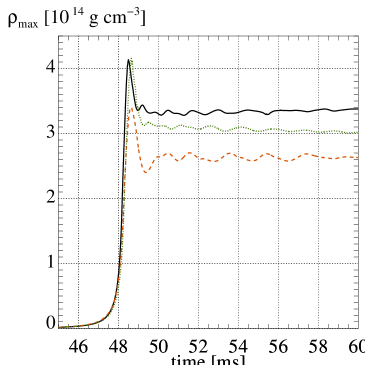
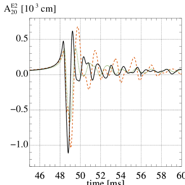
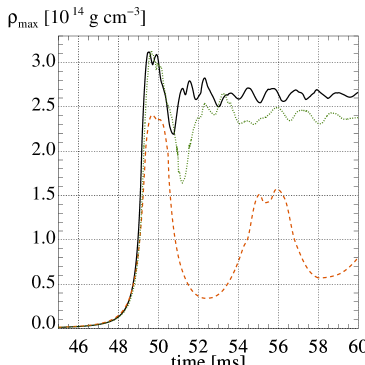
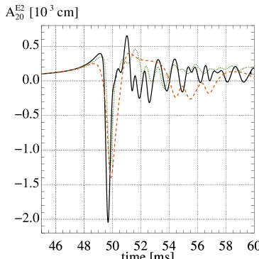
Figure 1: Evolution of the maximum density $\rho_{\mathrm{max}}$ (left panels) and the GW amplitude $A^{E2}_{20}$ (right panels) of models A1B3G3 (upper panels) and A3B3G3 (lower panels) computed with the Newtonian (dashed red lines) and the effective TOV (solid black lines) potential, and in full GR (dotted green lines) assuming CFC. A color version of the figure can be found in the on-line edition of the journal.

We also test the performance of the TOV potential in axisymmetric simulations of non-magnetic, rotating models using two prototypical models from the model set of Paper I (Table 4, Fig. 1).

Model A1B3G3 bounces both in Newtonian and GR gravity due to the stiffening of the equation of state beyond nuclear density (type I model). Using the effective TOV potential, the model reaches a maximum density at bounce, which is about 20 % higher than in the Newtonian case and only 2 % lower than in GR. The GW signal obtained with the effective TOV potential shows similar qualitative features as the one calculated in GR, but overestimates the signal amplitudes at bounce by about 50 % (Fig. 1, upper left). Using the Newtonian potential, the deviations are of comparable order, but persist also during the ring-down phase. The frequencies of the ring-down oscillations are off by $\sim 30\,\%$ in the Newtonian case, while those resulting from the effective TOV potential agree very well with the frequencies of the GR model.

Model A3B3G3 rotates initially quite differentially and very rapidly ($\beta_{\mathrm{rot}}^{\mathrm{ini}}=1.8\,\%$). In the Newtonian case, the core bounces mainly due to centrifugal forces, although it exceeds nuclear matter density during bounce. After bounce, the core expands to sub-nuclear densities and exhibits large-scale pulsations with little damping, giving rise to a GW signal intermediate to ZM’s type I and type II signals (Fig. 1, lower panels). In GR the core reaches a $\sim 40\,\%$ higher density during bounce and settles into a pressure supported equilibrium of supra-nuclear central density after some ring-down oscillations. The gravitational wave signal is of type I. The gross features of the GR density evolution are reproduced by the effective TOV potential, and the maximum density at bounce agrees within 5 % with that of the GR simulation. However, there are considerable differences in the GW signal. Contrary to the Newtonian potential, the TOV potential gives the correct signal type (I), but the amplitude of the dominant negative peak at bounce exceeds that of the Newtonian run by $\sim 30\,\%$, whereas the correct GR amplitude is $\sim 10\,\%$ smaller than the Newtonian one (Fig. 1, lower right).

The above results show that the TOV potential is able to reproduce the results of full GR simulations quite well for slowly rotating cores. For rapidly rotating models the evolution of the maximum density is reproduced very well, and the GW signal is of the correct type, but considerable differences are found concerning the amplitude of the GW signal. A more comprehensive investigation of the performance of effective TOV potentials in hydrodynamic simulations of rotational core collapse will be presented elsewhere (Müller et. al., in preparation).

3.2 Magnetohydrodynamic simulations

We consider four models from Paper I to explore the effects of relativistic gravity on the dynamics and the GW signal of magnetorotational core collapse. Three of these models exhibit the same type of signal as the corresponding Newtonian models of ZM: A1B3G3 (type I), A2B4G1 (type II), and A3B3G5 (type III). In the fourth model (A3B3G3), the GW signal changes from transition type I/II to type I when changing from Newtonian to relativistic gravity. For each of these selected models, we substitute the Newtonian potential by the effective TOV potential Eqs. (13, 14) and perform three MHD simulations with an initially weak ($10^{10}\ \mathrm{G}$), strong ($10^{12}\ \mathrm{G}$), and very strong magnetic field ($10^{13}\ \mathrm{G}$), respectively (see Figs. 2 to 7, and the tables in Appendix A).

Before we compare the results of the Newtonian versions of these MHD models (see Paper I) with those obtained with the effective TOV potential, we outline some relevant findings of Paper I. In Newtonian gravity, type I and type III models show a secular contraction when a strong initial magnetic field ($\ga 10^{12}\ \mathrm{G}$) is imposed, while the structure of the core remains unchanged from the hydrodynamic case. Type II models lose their centrifugal support and begin to depart from the rotational equilibrium established in the corresponding non-magnetic model. Eventually, they transform into a pressure supported configuration. All initially strongly magnetized models develop collimated bipolar outflows.

Overall, the MHD TOV models show the same qualitative dynamic behavior and the same GW signal types as the corresponding Newtonian ones, but they also exhibit several quantitative differences. The efficiency of the field amplification by winding due to differential rotation differs from the Newtonian case as the collapse proceeds to higher densities in the TOV models. This effect slightly shifts the borders between the various signal types in parameter space. As a consequence the new type IV GW signal, which was observed with the Newtonian potential for one single MHD model only (Paper I), is encountered more frequently when using the effective TOV potential.

Figure 2: The evolution of the maximum density (upper panels) and GW amplitudes (lower panels) of models A1B3G3-D3M10-N/T (left), A1B3G3-D3M12-N/T (middle), and A1B3G3-D3M13-N/T (right). Solid and dashed lines show TOV and Newtonian models, respectively.

Models of series A1B3G3-D3Mm-N/T show a qualitatively very similar behavior, but several small quantitative differences are observed. For the weak-field model A1B3G3-D3M10-T, both the maximum density at core bounce and in the post-bounce equilibrium state are larger than the corresponding Newtonian values by $\sim 25\,\%$ (Fig. 2, top left). The magnetic field is amplified by the differential rotation of the core in the same way as in the Newtonian case, and the TOV model also satisfies the MRI condition (Balbus & Hawley, 1991; Balbus, 1995; Akiyama et al., 2003) in large regions of the post-bounce core. The MRI growth times and saturation fields are of a similar order as in the Newtonian case, i.e. a few milliseconds and $\sim 10^{16}\ \mathrm{G}$, respectively (see also Paper I), but due to the faster rotation of the collapsed inner core, the growth times are slightly smaller and the saturation fields are slightly stronger than in the Newtonian case. The topologies and the energies of the magnetic field of the cores are quite similar in the post-bounce quasi-equilibrium state, the latter differing by only about 30 % at $t=89\,$ms ($E_{\mathrm{mag}}^{\mathrm{T}}=7.0\times 10^{51}\,$erg compared to $E_{\mathrm{mag}}^{\mathrm{N}}=9.8\times 10^{51}\,$erg). The magnetic field is predominantly toroidal, but also exhibits an additional complex structure consisting of cylindrical sheets and regions of field lines wound up like balls of wool. The GW amplitudes at bounce agree very well, the differences being smaller than 10 %, while the immediate post-bounce ring-down amplitudes are about 50 % smaller in the TOV model (Fig. 2, lower left). Concerning these results we point out that the evolution of the model in full GR is only approximated by the use of an effective TOV potential, and hence some additional, but probably small, modifications of the results are expected when repeating the simulations in full GR.

In the strong-field models A1B3G3-D3M12-T (Fig. 2, upper middle) and A1B3G3-D3M13-T (Fig. 2, upper right), considerable amounts of rotational energy are extracted from the central core by the transport of angular momentum caused by magnetic field stresses. Consequently, the core loses centrifugal support and begins to contract. This effect is qualitatively the same in Newtonian and TOV gravity, and with respect to the time scales, the amount of rotational energy lost, and the increase in the central density also are quantitatively very similar. The GW amplitude (Fig. 2, lower right) at bounce is enhanced by about 40 % compared to the non-magnetic or weak-field case (Fig. 2, lower left). The post-bounce GW signal shows the typical type I ring-down behavior superimposed on an initially rising ($t_{\mathrm{b}}\la t\la t_{\mathrm{b}}+5\,$ms) and then roughly constant positive mean GW amplitude. The later contribution to the GW signal is due to the emergence of a high speed ($v\sim{c}/{3}$) collimated outflow (jet) along the rotation axis.

As in the Newtonian case, the magnetic field of the initially most strongly magnetized model A1B3G3-D3M13-T already affects the angular momentum distribution of the core considerably during core collapse. At bounce the rotational energy of this core ($E_{\mathrm{rot}}^{\mathrm{T}}=4.2\times 10^{51}\,$erg) is lower by 18 % compared to that of models A1B3G3-D3M12-T and A1B3G3-D3M10-T ($E_{\mathrm{rot}}^{\mathrm{TOV}}=5.1\times 10^{51}\,$erg). In model A1B3G3-D3M12-T, the magnetic field is too weak at bounce to be dynamically important. However, a few milliseconds after bounce the poloidal field energy starts to grow exponentially when meridional circulation flow develops near the surface of the inner core. The flow winds up the radial magnetic field component, and magnetic stresses begin to transport angular momentum outwards. Furthermore, a weak bipolar outflow develops in this model towards the end of the simulation, which is driven primarily by magnetic hoop stresses. Because of this outflow, the GW amplitude rises slowly towards a positive mean value, which is however smaller than in the case of model A1B3G3-D3M13-T (Fig. 2, lower middle and right).

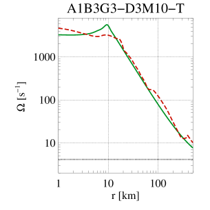
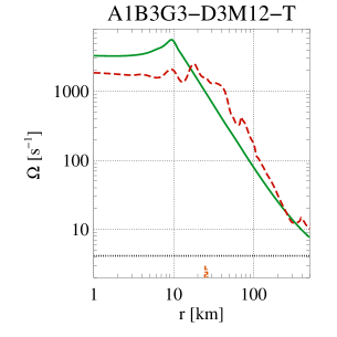
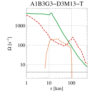
Figure 3: Temporal evolution of the rotation profiles for the models of series A1B3G3-D3Mm-T. The panels show the angular averaged profiles $\Omega(r)$ of models A1B3G3-D3M10-T (left), A1B3G3-D3M12-T (middle), and A1B3G3-D3M13-T (right), respectively. The initial rotation profiles and the profiles at core bounce are given by the black dotted and green solid lines, respectively. The additional lines show the profiles at $t\approx 65\,$ms, the red dashed and the orange dash-dotted lines corresponding to the angular averaged rotation profiles of the prograde and of the retrograde rotating parts of the core, respectively. While there is no region of retrograde rotation present in model A1B3G3-D3M10-T (left), and only a very small one in model A1B3G3-D3M12-T (middle), large amounts of matter rotate in a retrograde way near the equator in model A1B3G3-D3M13-T (right).

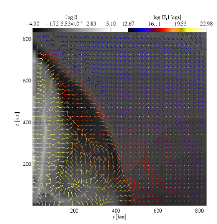
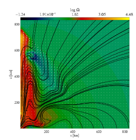
Figure 4: The left panel shows the distribution of $\beta=P_{\mathrm{mag}}/P_{\mathrm{gas}}$ in the outflow of model A1B3G3-D3M13-T at $t\approx 65\,$ms (grey scale) and the direction and modulus of the Lorentz force (arrows). The arrows are normalized to the same length, but show the strength of the force color-coded. The right panel displays the angular velocity distribution (color scale), the velocity field (arrows), and the magnetic field (field lines) at the same time.

To illustrate the effects of the magnetic field on the angular momentum distribution we compare the evolution of the angular averaged rotation profiles $\Omega(r)$ for three cores from our model series at different times (Fig. 3). Although rotating almost rigidly initially, all three cores develop a strongly differential rotation profile at bounce. At this evolutionary stage, there is only very little difference between the profiles of models A1B3G3-D3M10-T and A1B3G3-D3M12-T, whereas angular momentum transport by magnetic fields has already slightly altered the rotation profile of model A1B3G3-D3M13-T. At $t\approx 65\,$ms, the weak-field core still has essentially the same rotational profile as it had at bounce, while the the rotation profile of the strong-field cores has changed quite considerably. The rotation rate of the inner core of model A1B3G3-D3M12-T is down by a factor of $\sim 2$, and angular momentum transport by magnetic fields has created a fast rotating region outside of the inner core.

In the case of model A1B3G3-D3M13-T, angular momentum transport is even more efficient, and at intermediate radii, $7\,\mathrm{km}\la r\la 100\,\mathrm{km}$, a region of slow retrograde rotation develops near the equator. At similar radii, the fluid along the polar axis still rotates in a prograde direction but quite slowly, whereas the rotation rate of matter outside $\sim 70\,$km is much faster than in the corresponding models with weaker initial fields. Spatially, the rapidly rotating matter is concentrated along the axis in the jet-like outflow driven by the magnetic fields.

The differences between the rotation profiles reflect different modes of angular momentum redistribution to some extent. When amplified by compression during collapse, the initially strong field in model A1B3G3-D3M13-T manages to launch a prominent outflow, which carries angular momentum away from the center towards the outflow axis. In the less strongly magnetized model A1B3G3-D3M12-T, on the other hand, most transport is due to the magnetic field growing near the boundary of the inner core ($r\approx 20\,\mathrm{km}$) at all latitudes by the action of MHD instabilities. A few vortices develop, where the off-diagonal Maxwell-stress components responsible for angular momentum transport become large. Consequently, a considerable loss of rotational energy from the inner core occurs due to these vortices that extend further outwards with time. Only later in the evolution the appearance of a weak polar outflow opens up an additional channel of angular momentum transport similar to the one discussed above.

The efficient transport of angular momentum along the outflow and the collimation of the fluid by magnetic stresses together give rise to the very characteristic structure of the outflow (Fig. 4). The outflow drags along and bends the poloidal field lines that are initially located near the surface of the core, giving rise to the formation of a cylindrically shaped magnetic sheet (Fig. 4). This magnetic sheet separates the outflow into two concentric regions: an interior region resembling the beam of a jet and an exterior region resembling the jet cocoon. The fluid is collimated mainly by the magnetic field and predominantly by its hoop stress. Fig. 4 (left panel) shows the ratio $\beta\equiv P_{\mathrm{mag}}/P_{\mathrm{gas}}$ of the magnetic pressure and the gas pressure, as well as the direction and magnitude of the Lorentz force exerted by the magnetic field on the gas. The outflow is magnetically dominated, $\beta$ being much larger than unity. Regions of differently oriented Lorentz force can be identified, which gives rise to the formation of two regions, contractive and expansive, in the outflow that roughly match the division into beam (contractive) and cocoon (expansive) as sketched above. This feature appears to be inherent to the evolution of magnetized jets (see, e.g., Leismann et al. (2005)). As the gas is compressed towards the rotational axis, both the field strength and the angular velocity increase, i.e, the gas in the jet beam begins to rotate very rapidly (see Fig. 4, right panel).

Figure 5: The evolution of the maximum density (upper panels) and GW amplitudes (lower panels) of models A3B3G5-D3M10-N/T (left), A3B3G5-D3M12-N/T (middle), and A3B3G5-D3M13-N/T (right). Solid and dashed lines show TOV and Newtonian models, respectively.

Figure 6: The evolution of the maximum density (upper panels) and GW amplitudes (lower panels) of models A3B3G3-D3M10-N/T (left), A3B3G3-D3M12-N/T (middle), and A3B3G3-D3M13-N/T (right). Solid and dashed lines show TOV and Newtonian models, respectively.

Figure 7: The evolution of the maximum density (upper panels) and GW amplitudes (lower panels) of models A2B4G1-D3M10-N/T (left), A2B4G1-D3M12-N/T (middle), and A2B4G1-D3M13-N/T (right). Solid and dashed lines show TOV and Newtonian models, respectively.

The next series of models to be discussed is A3B3G5-D3Mm. Simulating these type III models with the effective TOV potential significantly changes neither the dynamics nor the GW signal compared to runs performed with the Newtonian potential (Fig. 5). The TOV models reach a slightly higher rotation rate than the corresponding Newtonian ones, which leads to a slightly more efficient amplification of the magnetic field. At 14 ms post bounce, the total magnetic energies of the Newtonian and TOV cores are $E_{\mathrm{mag}}^{\mathrm{N}}=3.8\times 10^{46}\,$erg, and $E_{\mathrm{mag}}^{\mathrm{TOV}}=6.0\times 10^{46}\,$erg, respectively. For models with a sufficiently strong magnetic field, the maximum density of the core increases like in the Newtonian case as the core loses rotational support due to the redistribution of angular momentum by magnetic field stresses. In model A3B3G5-D3M13-T the maximum density reached in the post-bounce quasi-equilibrium configuration is about 20 % higher than in the corresponding Newtonian model (Fig. 5, upper right). This statement also roughly holds for the weak-field model A3B3G5-D3M10 (Fig. 5, upper left; but note the different evolution of the maximum density for models with weak and strong initial magnetic fields). The type III GW signals of all three magnetized models are quite similar for the Newtonian and the effective TOV potential (Fig. 5, lower panels).

For the third series of models, A3B3G3-D3Mm, the changes resulting from the use of the effective TOV potential instead of the Newtonian one depend on the strength of the initial magnetic field (Fig. 6). The weak-field Newtonian model A3B3G3-D3M10-N, which bounces due to a combination of (mainly) centrifugal and pressure forces at $\rho_{\mathrm{b}}=2.4\times 10^{14}\ \mathrm{g\,cm}^{-3}$ just above nuclear matter density, shows several distinct post-bounce oscillations of the maximum density (Fig. 6 upper left) and emits a GW signal intermediate between a type I and a type II signal (Fig. 6, lower left). With the effective TOV potential, the model collapses deeper ($\rho_{\mathrm{b}}=3.1\times 10^{14}\ \mathrm{g\,cm}^{-3}$), thus spinning faster than in the Newtonian case. Its GW signal is almost a pure type I signal showing the typical ring-down oscillations instead of coherent large-scale oscillations (Fig. 6, lower left). The with stronger initial fields (A3B3G3-D3M12-T and A3B3G3-D3M13-T) collapse to about 30 % higher densities than their Newtonian counterparts. The initial magnetic fields of these models are sufficiently strong for both potentials to trigger a secular contraction of the core, due to angular-momentum redistribution by magnetic field stresses, and to cause a collimated outflow.

The cores of the fourth series of models (A2B4G1-D3Mm) considered in our study bounce due to centrifugal forces as do their Newtonian counterparts (and the GR-CFC models, see DFM) exhibiting multiple bounces and large-scale pulsations (Fig. 7). In the weak-field case (A2B4G1-D3M10-T), the maximum density never exceeds nuclear matter density, and the magnetic field is amplified less efficiently than in the models of series A1B3G3-D3Mm-T due to the longer rotation period of the less compact core of the models of series A2B4G1-D3Mm-T. Compared to the corresponding Newtonian model, we find a much higher field amplification rate. Both $E_{\mathrm{rot}}$ and $\beta_{\mathrm{mag}}$ have about the same magnitude in the TOV model at bounce as the corresponding quantities in the Newtonian model about 50 ms past bounce (during the second pulsation of the core centered at $t\approx 150\,$ms), i.e. after a significantly longer period of amplification. This is a consequence of the deeper collapse of the TOV model, whose maximum density exceeds that of the Newtonian model A2B4G1-D3M10-N by a factor of about seven (Fig. 7, upper left). This, in turn, leads to a more compact core with a shorter rotation period favoring a more efficient field amplification. The core emits a type II GW signal like the Newtonian counterpart (Fig. 7, lower left).

The effects of a strong magnetic field on models of series A2B4G1-D3Mm-T are even more pronounced than in the Newtonian case due to the deeper relativistic potential. For an initial field of $\sim 10^{13}\ \mathrm{G}$ the Newtonian model exhibits one small amplitude pulsation (centered at $\sim 110\,$ms) before angular-momentum transport induced by the magnetic field triggers a rapid contraction at $\sim 140\,$ms (Fig. 7, upper right). The dynamic impact of a field of $\sim 10^{12}\ \mathrm{G}$ on the core of the TOV model is very similar to that of a field of $\sim 10^{13}\ \mathrm{G}$ in the Newtonian case. Both cores (A2B4G1-D3M12-T and A2B4G1-D3M13-N) undergo one single post-bounce pulsation, where the amplitude is more pronounced in the TOV model (Fig. 7, upper middle and right), and then rapidly contract to densities slightly above nuclear matter density ($\rho_{\mathrm{max}}\approx 2.7\times 10^{14}\ \mathrm{g\ cm^{-3}}$).

During the immediate post-bounce evolution, the GW signals emitted by the strong field models are very similar to those of the weak-field model A2B4G1-D3M10-T. However, later in the evolution, the GW signals are radically different from those of the corresponding non-magnetic and initially weakly magnetized cores (Fig. 7, lower panels). For $t\ga 130\,$ms, the GW amplitude of model A2B4G1-D3M12-T exhibits rapid oscillations with periods in the range of milliseconds (Fig. 7, lower middle), while it rises to high positive values in the case of model A2B4G1-D3M13-T at $t\approx 115\,$ms (Fig. 7, lower right) also showing superimposed oscillations. The frequency of the oscillations increases as the density of the core grows. When it reaches supra-nuclear densities, we observe oscillation periods in the sub-millisecond range and oscillation amplitudes on the order of 100 cm. The large positive amplitude ($\sim 900\,$cm) of model A2B4G1-D3M13-T at late times is due to the very prolate shape of its shock wave (jet).

As the GW signals of models A2B4G1-D3M12-T and A2B4G1-D3M13-T do not belong to any of the familiar types I, II, or III, we classify them as belonging to a new (magnetic) type IV GW signal, introduced in Paper I.

Finally, we discuss the process of shock formation in model A2B4G1-D3M13-T in some more detail, which is also relevant to models A2B4G1-D3M12-T and A2B4G1-D3M13-N. In a type I model, the shock forms by the steepening of pressure waves created as successive shells of core matter feel the stiffening of the equation of state during bounce. The pressure waves move outwards and evolve into a shock as they accumulate near the sonic point. The typical time scale for this process is on the order of the sound-crossing time of the inner core (that part of the core that is located inside the sonic point), which is approximately 1 ms. In contrast, the shock wave is launched in a type II model at the edge of the inner core, when it bounces due to the effect of the centrifugal force and expands into the still infalling matter of the outer core with supersonic speed. The strength of this shock may vary strongly with polar angle and may even develop for different angles at different times.

Both modes of shock generation are at work in model A2B4G1-D3M13-T. During its collapse the rotational energy rises considerably, but less than in the non-magnetic or weak-field case. The rotation rate $\beta_{\mathrm{rot}}$ already reaches a maximum during collapse when $\rho_{\mathrm{max}}=8.4\times 10^{13}\,\mathrm{g\,cm}^{-3}$, i.e. well below the bounce density $\rho_{\mathrm{b}}=3.5\times 10^{14}\,\mathrm{g\,cm}^{-3}$, as very efficient angular momentum transport by the strong magnetic fields extracts rotational energy from the core. This effect creates a rotation profile in the core where matter with the same density as in the corresponding non-magnetic or weakly magnetized models rotates faster near the pole. The extraction of rotational energy from the inner core also causes the post-shock gas to continue to fall towards the center, and further shock waves are created by the pressure-bounce mechanism.

Two shock waves form at high latitudes near the surface of the inner core (at $r\approx 100\,$km and $r\approx 140\,$km; see Fig. 8, upper left, last snapshot), while matter near the equator is still falling in. No shock is present there yet (Fig. 8, lower left). About 5 ms later at $t\approx 110\,$ms a third polar shock (at $r\approx 30\,$km; see Fig. 8, upper middle, first snapshot) and an equatorial shock (at $r\approx 130\,$km; see Fig. 8, lower middle, first snapshot) have formed. The second polar shock, which is stronger and propagates faster than the first one, is about to merge with it about 6 ms later at $t\approx 116\,$ms (Fig. 8, upper right, first snapshot). Two more polar shock and one additional equatorial one form up until the end of our simulation at $t\approx 118\,$ms (about 10 ms after bounce), when the first and second polar and equatorial shocks have merged, and are located at a radius of $r_{\mathrm{p}}\approx 410\,$km along the polar direction and $r_{\mathrm{e}}\approx 310\,$km along the equator, respectively (Fig. 8, right, last snapshots). The creation and propagation of the various shock waves gets imprinted on the density distribution, which is strongly anisotropic and exhibits several distinct discontinuities, their number and radial location depending on polar angle.

In the corresponding weak-field core, we find an almost isotropic expansion of the post-shock matter supported by centrifugal forces. At $t\approx 109\,$ms the nearly spherically symmetric, leading shock wave has reached a polar and equatorial radius of $r_{\mathrm{p}}\approx 320\,$km and $r_{\mathrm{e}}\approx 300\,$km, respectively. The density distribution is almost spherical and shows much less structure than in the strong-field case.

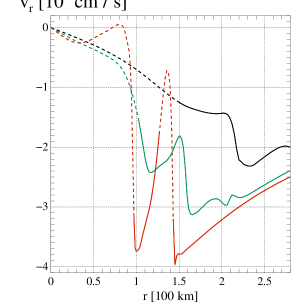
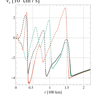
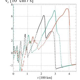
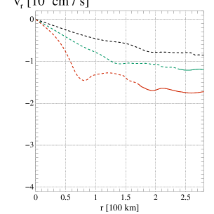
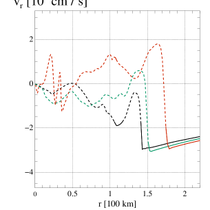
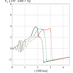
Figure 8: Radial velocity profiles for the strong-field model A2B4G1-D3M13-T along the rotation axis (top) and at the equator (bottom) at different epochs. Each panel shows three snapshots, plotted in black, green, and red. Solid and dashed lines mark subsonic and supersonic radial motion, respectively. The snapshots are taken at $t=94.8,100.4,105.0\,$ms (left), $t=110.0,110.7,112.3\,$ms (middle), and $t=115.9,117.0,117.9\,$ms (right). A color version of the figure can be found in the on-line edition of the journal.

3.3 Gravitational wave spectra

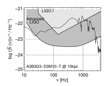
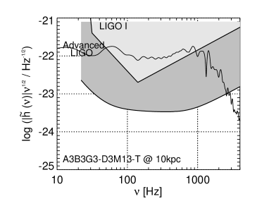
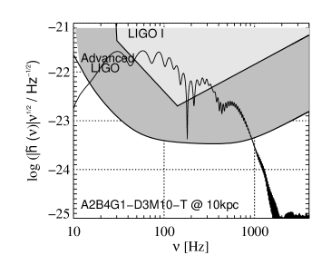
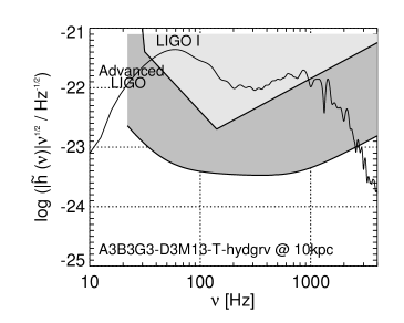
Figure 9: The GW spectral energy distribution $|\tilde{h}(\nu)|\nu^{1/2}|$ of a weak-field (A3B3G3-D3M10-T, upper left) and strong-field (A3B3G3-D3M13-T, upper right) model bouncing due to pressure forces, and of a weak-field (A2B4G1-D3M10-T, middle left) and strong-field (A2B4G1-D3M13-T, middle right) model bouncing due to centrifugal forces. The magnetic and non-magnetic contributions to the GW amplitude of model A3B3G3-D3M13-T are displayed in the lower left and right panels, respectively. The grey-shaded regions give the detection limits of the current (LIGO I) and the Advanced LIGO interferometer. The source is assumed to be located at a distance of 10 kpc.

We also calculate the spectral energy distribution $|\tilde{h}(\nu)|\nu^{1/2}$ of the gravitational wave signals emitted by our models. The Fourier-transformed amplitudes $\tilde{h}(\nu)$ as a function of the signal frequency $\nu$ are obtained from the GW signals $h(t)$ using fast Fourier transforms (for details, see e.g. Müller et al., 2004).

Spectra of non-magnetic models were already discussed by Dimmelmeier et al. (2002b). Typical GW spectra of type I (A3B3G3-D3M10-T) and type II (A2B4G1-D3M10-T) models are shown in Fig. 9 for a source located at a distance of 10 kpc. The GW spectrum of a type I model peaks at high frequencies ($\sim 800\,$Hz), whereas the spectrum of a multiple bounce (type II) model possesses a very broad maximum at frequencies of $\sim 30-200\,$Hz, reflecting the different bounce mechanisms of the inner cores of the two models. In the former case, the core is very compact, and thus having a short dynamic time scale of a few milliseconds, leading to rapid ring-down oscillations and a high-frequency signal. The multiple centrifugal bounces of model A2B4G1-D3M10-T recurring on comparatively long time scales of $\sim 35\,$ms cause the low-frequency maximum in the spectrum. This difference is also present in a comparison of the spectra of the Newtonian and the TOV version of model A3B3G3-D3M10. The spectrum of the Newtonian model, being of transition type I/II, peaks at considerably lower frequencies ($\sim 150-500\,$Hz) than the one computed with the effective TOV potential ($\ga 400\,$Hz). Most of the weak-field models are marginally detectable with the LIGO interferometer for a source located at a distance of 10 kpc.

At very low-frequencies, the characteristic modification imprinted onto the GW spectrum by strong magnetic fields is a dominant feature. The main differences between weak-field and strong-field versions of a given model are visible in the low frequency range for type I models, while the high-frequency part is affected relatively modestly. Model A3B3G3-D3M13-T has a considerable excess of spectral power at frequencies $\la 100\,$Hz compared to model A3B3G3-D3M10-T. In contrast to the latter, the spectrum of model A3B3G3-D3M13-T is flat at frequencies below the peak frequency $\sim 800\,$Hz. This feature can be attributed to the jet-like outflow, giving rise to a strongly positive GW amplitude of slow temporal variability. Both the magnetic and the non-magnetic contributions to the GW amplitudes have strong low-frequency contributions reflecting how the outflow is neither purely magnetic nor purely hydrodynamic, but of a magnetohydrodynamic nature. Note that the magnetic and non-magnetic contributions to the spectrum may have different signs. Therefore, the total spectral power is suppressed by a factor of $\sim 2.5$ with respect to both contributions. For a source at a distance of 10 kpc, the flatter spectrum of the strong-field model improves its detectability with the laser interferometers such as the LIGO detector. The high-frequency part of the spectrum, as well as the frequency and amplitude of the peak in the spectrum are insensitive to the magnetic field.

For multiple-bounce (type II) models there is a substantial difference between weak-field and strong-field versions both at low frequencies (like in type I models) and high frequencies. A particularly good example for such a difference are the models of series A2B4G1-D3Mm-T, ranging from the weak-field type II model A2B4G1-D3M10-T to the type IV model A2B4G1-D3M13-T. Unlike the spectrum of the former model with its broad low-frequency maximum and a rapid decrease towards high frequencies, the spectral energy distribution of model A2B4G1-D3M13-T has a rather strong contribution above $\sim 700\,$Hz. At a frequency of $\approx 1500\,$Hz the latter signal has about 10 times more power than the former one. This part of the spectrum is produced by the very rapid oscillations of the core as it collapses to nuclear matter density, and the dynamical time scale drastically decreases.

4 Summary and conclusions

We have presented an investigation of the gravitational collapse of rotating magnetized stellar cores including an approximate relativistic TOV potential to mimic the effects of general relativity in our simulations. The implementation of this potential requires only minor modifications of an existing Newtonian MHD code and provides a good approximation to full GR dynamics in the case of the collapse of a stellar core to a neutron star. In particular, we are able to reproduce the change in the bounce mechanism (centrifugal vs. pressure) occurring in some (non-magnetic, rotating) models when changing from Newtonian to GR gravity. The maximum densities obtained with the approximate relativistic TOV potential are, as expected, higher than the corresponding Newtonian ones. This also holds for the rotational energies, although some exceptions exist to this rule. The gravitational wave signals exhibit the same qualitative behavior as in full GR, but they differ quantitatively.

Comparing the results obtained with the approximate TOV potential with those of our previous Newtonian calculations of the magneto-rotational collapse of stellar cores (described in detail in Paper I), we find that the main difference corresponds to a “shift” in the parameter space. In TOV gravity, one needs faster or more differential rotation to cause centrifugal effects of similar strength for the same equation of state. Given the same initial model and the same equation of state, a core in TOV gravity will collapse to higher densities. This deeper collapse of the TOV model leads in many of our models to a faster rotation of the inner core than in the corresponding Newtonian case, causing a more efficient amplification of the magnetic field by differential rotation ($\Omega$ dynamo). In principle, an $\alpha$-$\Omega$-type dynamo could develop due to differential rotation and possible 3D MHD instabilities, as in the Newtonian case (Spruit, 2002). However, in our axisymmetric simulations, the transformation of toroidal into poloidal fields is suppressed, hence we are unable to simulate this kind of dynamo.

We find that the magneto-rotational instability can develop in the TOV models as well as in the Newtonian ones. The growth times and saturation fields of the magnetic fields resulting from the MRI are within the same order of magnitude as in the Newtonian case, i.e. in the range of milliseconds and $\ga 10^{15}\,\mathrm{G}$, respectively. Due to the grid-resolution problem already discussed for the Newtonian models (see Paper I), we are unable to simulate the evolution of the MRI unless the seed field is already quite strong. In models belonging to the latter class, we find an exponential growth of the poloidal field of the inner core during the post-bounce evolution by the action of the MRI.

The influence of strong magnetic fields on the dynamics and the GW signal of the core by braking its rotation and thus triggering a post-bounce contraction is aided by the deeper TOV potential. For type II multiple bounce models, we find that magnetic fields affect the dynamics and GW signal of the core by a similar amount to what is observed for Newtonian models with a considerably (i.e. $\sim 10$ times) stronger initial magnetic field.

For the most extreme type II model (A2B4G1-D3M13-T), the rotation rate $\beta_{\mathrm{rot}}$ already decreases during the final stages of the initial core collapse. When the rotation rate reaches its maximum value of about 12%, a centrifugally supported shock wave is launched that fails to explode the core. The core continues to collapse and eventually bounces at supra-nuclear densities due to the stiffening of the equation of state. The GW signal of this model belongs to the magnetic-type GW signal (type IV) introduced in Paper I. At early epochs it resembles a type II signal, but after the launch of the first shock it shows quite a different nature. Instead of the long-period oscillations characteristic of a type II signal, the GW amplitude shows violent oscillations whose frequencies increase as the local sound-crossing time scale decreases in the core when it collapses to nuclear matter density. Such a signal is also produced by a less magnetized TOV model of the same model series (A2B4G1-D3M12-T) and by the corresponding strongly magnetized Newtonian model (A2B4G1-D3M13-N).

In some of our models we observe that the GW signal exhibits an almost constant positive amplitude towards the end of the respective simulations (see, e.g. model A3B3G3-D3M13-T/N), or it oscillates around a positive value (see, e.g. model A3B3G5-D3M13-T/N). This is due to the presence of the jet-like outflow along the rotation axis in those models. It is tempting to interpret this behavior of the GW signal as a “burst with memory” (Braginsky & Thorne, 1987), as suggested by T. Pradier (private communication), which results e.g. when a blob of matter that is initially at rest is accelerated during some time interval and moves at a constant speed afterwards, giving rise to a non-vanishing constant gravitational wave amplitude (see, e.g. Segalis & Ori, 2001). However, we do not think that the GW signals of our models show a “memory” effect. The almost constant GW amplitude in some models is a transient resulting from the combined action of a decelerating jet-like outflow and the related magnetic contributions to the total quadrupole moment.

Appendix A Synopsis of our results

Tables 5 and 6 provide an overview of the dynamic evolution of the flow and the magnetic field and include information on the resulting gravitational wave signal of all our models.

Table 5: Some characteristic model quantities.

Model	Type	$t_{\mathrm{b}}$ a	$\rho_{\mathrm{b,14}}$ b	$A^{\mathrm{E}2}_{20}$ c	$A^{\mathrm{E}2}_{20;\mathrm{mag}}$ d	$A^{\mathrm{E}2}_{20;\infty}$ e	$\beta_{\mathrm{rot}}^{\mathrm{max}}$ f	$\beta_{\mathrm{mag}}^{\mathrm{max}}$ g	$t_{\mathrm{m}}$ h	$\beta_{\mathrm{mag};\phi}^{\mathrm{max}}$ i
		$[\mathrm{ms}]$		$[\mathrm{cm}]$	$[\mathrm{cm}]$	$[\mathrm{cm}]$	[%]	[%]	$[\mathrm{ms}]$	[%]
A1B3G3-D3M10-T	I	$48.5$	$4.13$	$-1110$	$0.005$	$40$	$7.3$	$0.01$!	$85.1$	$0.01$
A1B3G3-D3M12-T	I	$48.5$	$4.14$	$-1129$	$22$	$80$	$7.3$	$1.3$	$62.1$	$1.1$
A1B3G3-D3M13-T	I	$49.6$	$4.15$!	$-1474$	$39$	$400$	$6.1$	$2.8$	$54.4$	$1.5$
A2B4G1-D3M10-T	II	$101$	$0.70$	$-673$	$0.008$	—	$15.9$	$0.0003$!	$169$	$0.0003$
A2B4G1-D3M12-T	IV	$101$	$0.72$!	$-667$	$43$	—	$15.8$	$0.8$!	$140$	$0.7$
A2B4G1-D3M13-T	IV	$111$	$0.98$	$923$	$184$	—	$11.7$	$4.3$	$113$	$3.1$
A3B3G3-D3M10-T	I	$49.5$	$3.12$	$-2044$	$0.009$	$100$	$17.1$	$0.009$!	$80.6$	$0.009$
A3B3G3-D3M12-T	I	$49.5$	$3.13$!	$-2079$	$44$	$100$	$16.9$	$1.5$	$50.6$	$1.3$
A3B3G3-D3M13-T	I	$51.1$	$3.31$!	$-1584$	$524$	$700$	$13.9$	$4.3$	$53.6$	$2.9$
A3B3G5-D3M10-T	III	$30.4$	$3.69$	$272$	$10^{-5}$	$10$	$10.0$	$0.002$!	$72.6$	$0.002$
A3B3G5-D3M12-T	III	$30.4$	$3.69$	$274$	$-0.04$	$0$	$10.0$	$0.6$!	$38.2$	$0.5$
A3B3G5-D3M13-T	III	$30.5$	$3.69$!	$350$	$-35$	$100$	$9.4$	$5.2$	$35.1$	$2.8$

• Time of bounce.

• Maximum density at bounce (in units of $10^{14}\mathrm{g\,cm}^{-3}$). A density value with an exclamation mark indicates that the maximum density of the model exceeds the bounce density during the later evolution.

• Maximum GW amplitude.

• Magnetic contribution to the maximum GW signal

• A rough mean value of the wave amplitude (in cm) at some late epoch; no value is provided when the amplitude does not approach a quasi-constant asymptotic value. A large absolute value of this amplitude indicates the presence of an aspheric outflow.

• Maximum value of the ratio of rotational to gravitational energy.

• Maximum value of the ratio of magnetic to gravitational energy. An exclamation mark indicates that the magnetic field is still growing at the end of the simulation.

• The time when $\beta_{\mathrm{mag}}$ reaches its maximum value.

• Maximum value of the ratio of toroidal magnetic to gravitational energy.

Table 6: Some characteristic model quantities (name of model given in column 1) when the core has reached a quasi-equilibrium state.

Model	$t$ a	$r_{\mathrm{c}}$ b	$M_{\mathrm{c}}$ c	${2\pi}/{\Omega}$ d	$|\@vec{b}|$ e	$|b_{\phi}|$ f	$r_{\mathrm{sh}}^{\mathrm{p}}$ g	$r_{\mathrm{sh}}^{\mathrm{e}}$ h
	$[\mathrm{ms}]$	$[\mathrm{km}]$	$[{M_{\odot}]}$	$[\mathrm{ms}]$	$[\mathrm{G}]$	$[\mathrm{G}]$	$[\mathrm{km}]$	$[\mathrm{km}]$
A1B3G3-D3M10-T	$70$	$19.7$	$0.58$	$4.2$	$7.1\times 10^{13}$	$7.0\times 10^{13}$	$528$	$471$
A1B3G3-D3M12-T	$70$	$19.6$	$0.56$	$3.2$	$1.6\times 10^{15}$	$1.2\times 10^{15}$	$549$	$490$
A1B3G3-D3M13-T	$70$	$18.0$	$0.60$	$-1631$	$2.9\times 10^{15}$	$2.3\times 10^{14}$	$1170$	$563$
A2B4G1-D3M10-T	$167$	$134$	$1.26$	$34$	$9.8\times 10^{10}$	$8.5\times 10^{10}$	—	—
A2B4G1-D3M12-T	$141$	$45.3$	$0.97$	$9.0$	$2.7\times 10^{14}$	$2.6\times 10^{14}$	—	—
A2B4G1-D3M13-T	$129$	$23.9$	$0.91$	$139$	$1.9\times 10^{15}$	$3.4\times 10^{14}$	—	—
A3B3G3-D3M10-T	$68$	$22.0$	$0.64$	$3.8$	$9.1\times 10^{13}$	$9.1\times 10^{13}$	$532$	$427$
A3B3G3-D3M12-T	$68$	$25.5$	$0.55$	$9.4$	$6.7\times 10^{14}$	$5.6\times 10^{14}$	$545$	$458$
A3B3G3-D3M13-T	$68$	$23.0$	$0.54$	$28$	$1.3\times 10^{15}$	$3.9\times 10^{14}$	$1008$	$590$
A3B3G5-D3M10-T	$50$	$12.6$	$0.19$	$3.0$	$4.0\times 10^{13}$	$4.0\times 10^{13}$	$241$	$241$
A3B3G5-D3M12-T	$41$	$10.9$	$0.17$	$2.4$	$4.1\times 10^{15}$	$3.9\times 10^{15}$	$144$	$144$
A3B3G5-D3M13-T	$50$	$13.0$	$0.24$	$-31$	$3.5\times 10^{15}$	$1.2\times 10^{14}$	$822$	$329$

• Time at which the quantities given were determined. For the models of series A2B4G1-D3Mm-T, which do not reach a quasi-equilibrium state by the end of the simulation, we provide the corresponding quantities for the final model of the respective simulation.

• The surface radius of the gravitationally bound quasi-equilibrium configuration. Since it is still surrounded by an (expanding) envelope of high density matter, the definition of its surface radius $r_{\mathrm{c}}$ is somewhat uncertain.

• The mass of the gravitationally bound quasi-equilibrium configuration.

• The rotation rate at the surface. The angular velocity $\Omega$ is averaged over the angle $\theta$. Note that this quantity varies strongly and on short time scales near the surface. Thus, the values provided should be used with care. Negative values of the rotation rate signify counter-rotating cores.

• The total magnetic field at the surface. Note that this quantity varies strongly and on short time scales near the surface. Thus, the values provided should be used with care.

• The toroidal magnetic field at the surface. Note that this quantity varies strongly and on short time scales near the surface. Thus, the values provided should be used with care.

• The radius of the shock wave at the polar axis. No entry here implies that the shock has already left the computational grid.

• The radius of the shock wave at the equator. No entry here implies that the shock has already left the computational grid.

References

- Akiyama et al. (2003) Akiyama, S., Wheeler, J. C., Meier, D. L., & Lichtenstadt, I. 2003, ApJ, 584, 954
- Ardeljan et al. (2005) Ardeljan, N. V., Bisnovatyi-Kogan, G. S., & Moiseenko, S. G. 2005, MNRAS, 359, 333
- Balbus (1995) Balbus, S. A. 1995, ApJ, 453, 380
- Balbus & Hawley (1991) Balbus, S. A. & Hawley, J. F. 1991, ApJ, 376, 214
- Bisnovatyi-Kogan et al. (1976) Bisnovatyi-Kogan, G. S., Popov, I. P., & Samokhin, A. A. 1976, Ap&SS, 41, 287
- Braginsky & Thorne (1987) Braginsky, V. B. & Thorne, K. S. 1987, Nature, 327, 123
- Buras et al. (2003) Buras, R., Rampp, M., Janka, H.-T., & Kifonidis, K. 2003, Phys. Rev. Lett., 90, 241101
- Dimmelmeier et al. (2002a) Dimmelmeier, H., Font, J. A., & Müller, E. 2002a, A&A, 388, 917
- Dimmelmeier et al. (2002b) Dimmelmeier, H., Font, J. A., & Müller, E. 2002b, A&A, 393, 523
- Evans & Hawley (1988) Evans, C. R. & Hawley, J. F. 1988, ApJ, 332, 659
- Janka et al. (2005) Janka, H.-T., Buras, R., Kifonidis, K., Marek, A., & Rampp, M. 2005, in Cosmic Explosions, On the 10th Anniversary of SN1993J. Proceedings of IAU Colloquium 192. Edited by J.M. Marcaide and Kurt W. Weiler. Springer Proceedings in Physics, vol. 99. Berlin: Springer, 2005, p.253, 253
- Janka et al. (2004) Janka, H.-T., Buras, R., Kitaura Joyanes, F., Marek, A., & Rampp, M. 2004, in Proceedings of the 12th workshop on ”Nuclear Astrophysics”: A tribute to an explosive astrophysicist honoring Wolfgang Hillebrandt on occassion of his 60th birthday, ed. E. Müller & H.-T. Janka (Max-Planck-Institut für Astrophysik, Garching bei München, Germany), 150–160
- Janka et al. (1993) Janka, H.-T., Zwerger, T., & Mönchmeyer, R. 1993, A&A, 268, 360
- Jin & Xin (1995) Jin, S. & Xin, Z. 1995, Commun. Pure Appl. Math., 38, 235
- Komatsu et al. (1989) Komatsu, H., Eriguchi, Y., & Hachisu, I. 1989, MNRAS, 237, 355
- Kotake et al. (2004a) Kotake, K., Sawai, H., Yamada, S., & Sato, K. 2004a, ApJ, 608, 391
- Kotake et al. (2005) Kotake, K., Yamada, S., & Sato, K. 2005, ApJ, 618, 474
- Kotake et al. (2004b) Kotake, K., Yamada, S., Sato, K., et al. 2004b, Phys. Rev. D, 69, 124004
- LeBlanc & Wilson (1970) LeBlanc, J. M. & Wilson, J. R. 1970, ApJ, 191, 541
- Leismann et al. (2005) Leismann, T., Antón, L., Aloy, M. A., et al. 2005, A&A, 436, 503
- Marek et al. (2006) Marek, A., Dimmelmeier, H., Janka, H. ., Mueller, E., & Buras, R. 2006, A&A, 445, 273
- Meier et al. (1976) Meier, D. L., Epstein, R. I., Arnett, W. D., & Schramm, D. N. 1976, ApJ, 204, 869
- Mezzacappa (2005) Mezzacappa, A. 2005, in ASP Conf. Ser. 342: 1604-2004: Supernovae as Cosmological Lighthouses, 175
- Mönchmeyer et al. (1991) Mönchmeyer, R., Schäfer, G., Müller, E., & Kates, R. E. 1991, A&A, 246, 417
- Müller & Hillebrandt (1979) Müller, E. & Hillebrandt, W. 1979, A&A, 80, 147
- Müller et al. (2004) Müller, E., Rampp, M., Buras, R., Janka, H.-T., & Shoemaker, D. H. 2004, Astrophys. J., 603, 221
- Müller & Steinmetz (1995) Müller, E. & Steinmetz, M. 1995, Comp. Phys. Comm., 89, 45
- Obergaulinger et al. (2006) Obergaulinger, M., Aloy, M. A., & Müller, E. 2006, A&A, in press; astro-ph/0510184
- Ohnishi (1983) Ohnishi, T. 1983, Tech. Rep. Inst. Atom. Energy, 198, Kyoto University
- Rampp & Janka (2002) Rampp, M. & Janka, H.-T. 2002, A&A, 396, 361
- Sawai et al. (2005) Sawai, H., Kotake, K., & Yamada, S. 2005, ArXiv Astrophysics e-prints (astro-ph/0505611)
- Segalis & Ori (2001) Segalis, E. B. & Ori, A. 2001, Physical Review, D64, 064018
- Shapiro & Teukolsky (1983) Shapiro, S. L. & Teukolsky, S. A. 1983, Black holes, white dwarfs, and neutron stars (Wiley, New York)
- Shibata & Sekiguchi (2005) Shibata, M. & Sekiguchi, Y.-I. 2005, Phys. Rev. D, 71, 024014
- Spruit (2002) Spruit, H. C. 2002, A&A, 381, 923
- Symbalisty (1984) Symbalisty, E. M. D. 1984, ApJ, 285, 729
- Takiwaki et al. (2004) Takiwaki, T., Kotake, K., Nagataki, S., & Sato, K. 2004, ApJ, 616, 1086
- Wheeler et al. (2002) Wheeler, J. C., Meier, D. L., & Wilson, J. R. 2002, ApJ, 568, 807
- Yamada & Sawai (2004) Yamada, S. & Sawai, H. 2004, ApJ, 608, 907
- Zwerger & Müller (1997) Zwerger, T. & Müller, E. 1997, A&A, 320, 209