A model for atomic and molecular interstellar gas:
The Meudon PDR code
Abstract
We present the revised “Meudon” model of Photon Dominated Region (PDR code), presently available on the web under the Gnu Public Licence at: http://aristote.obspm.fr/MIS. General organisation of the code is described down to a level that should allow most observers to use it as an interpretation tool with minimal help from our part. Two grids of models, one for low excitation diffuse clouds and one for dense highly illuminated clouds, are discussed, and some new results on PDR modelisation highlighted.
1 Introduction
The recognition of the importance of photodissociation processes and their relation to atomic to molecular transitions in interstellar clouds started with Bates & Spitzer (1951). However, the first numerical quantitative model computing the various atomic and molecular abundances was presented by Black & Dalgarno (1977). These authors focused their study on the diffuse cloud toward the bright star Oph described as a “standard” diffuse cloud for which extensive observational information was available, including the first detection of molecular hydrogen in various rotational levels derived from absorption transitions with the Copernicus satellite (Morton, 1975). Further impetus to study such environments has been provided on the one hand by the detection of infrared emission of molecular hydrogen, ionised and neutral carbon, neutral oxygen and the so called aromatic bands at 3.3, 7.6 and 11 . The availability of the facility cryogenic grating spectrometer with the 91cm telescope of the Kuiper Airborne Observatory has allowed to detect for the first time, the far infrared emission lines of [OI] (63, 146 ), [CII] (158 ), [SiII] (35 ), and excited rotational lines of CO in luminous galaxies, planetary and reflection nebulae. These observations have emphasized the importance of Photon Dominated Regions and were interpreted in the context of theoretical models such as those of Tielens & Hollenbach (1985a, b) and Le Bourlot et al. (1993a). The ISO (Infrared Space Observatory) observed bright nebulae such as in Orion (Abergel et al., 2003).
These almost neutral astrophysical regions where ultraviolet photons penetrate and affect the physical and chemical properties are described now as Photon Dominated Regions (PDRs). These include hot gas close to HII regions, diffuse and translucent clouds (Galactic and inter-galactic), and the envelopes of dark clouds where star formation takes place. They have been extensively described in the review article of Hollenbach & Tielens (1999). Additional impulse came after the launch of the FUSE (Far Ultraviolet Spectroscopic Explorer) satellite in 1999 which can detect and HD in absorption in a variety of Galactic and extragalactic environments (Rachford et al., 2002; Tumlinson et al., 2002; Bluhm et al., 2003; Boissé et al., 2005; Lacour et al., 2005). The perspective of Spitzer and Herschel reinforces the need to describe as accurately as possible the physical conditions of photon-dominated environments and clarify the possible diagnostics. Various groups have developed PDR codes at different stages of sophistication and a workshop has been held in the Lorentz Center in Leiden in March 2004 to make detailed comparisons between the different numerical codes. Roellig et al. (2005) describe the results obtained for different test cases.
The present paper delineates the recent implementations performed in our PDR model (Le Bourlot et al., 1993a), labelled as the “Meudon PDR code”, which is available at the address http://aristote.obspm.fr/MIS. The aim is to gather in a single paper the physical questions and the numerical answers which have been implemented so far and to provide to the observers a numerical tool to interpret their observations. We also want to emphasise remaining issues to consider, such as the inclusion of data and/or processes which are poorly known. The organisation of the paper is the following: Sects. 2 to 7 describe the physics and give technical details on the organisation of the code (2: general features, 3: grains, 4: radiative transfer, 5: excitation, 6: thermal balance, 7: chemistry). Some representative examples are found in Sect. 8 and 9, and Sect. 10 is our conclusion. Various appendices highlight more specific points.
2 General features
2.1 Overview
The model considers a stationary plane-parallel slab of gas and dust illuminated by an ultraviolet radiation field (described in Appendix C) coming from one or both sides of the cloud (the two intensities can be different). It solves, in an iterative way, at each point in the cloud, the radiative transfer in the UV taking into account the absorption in the continuum by dust and in discrete transitions of and . Explicit treatment is performed for and photoionisation, and photodissociation and (and its isotopomeres) predissociating lines. The model also computes the thermal balance taking into account heating processes such as the photoelectric effect on dust, chemistry, cosmic rays, etc. and cooling resulting from infrared and millimeter emission of the abundant ions, atoms and/or molecules. Chemistry is solved, and abundances of each species are computed at each point. The excitation state of a few important species is then computed. The program is then able to calculate column densities and emissivities/intensities.
One major restriction is the strict steady-state approximation, so that model results cannot be compared directly to observations of rapidly evolving regions. However, the time scales of photoprocesses are modest at lower extinction and/or high radiation fields and shorter than the typical two body chemical reaction time scale in diffuse environments. The time scale given by the photodissociation is typically years at the edge of a cloud (with the FUV radiation strength – see Sect 4.2). The steady state approximation is then satisfactory.
2.2 Variables and parameters
As modellers, we can define the parameters which describe the system and which can be tuned at our will. As a consequence, some variables will adjust themselves under those choices and the constraints of physical laws.
Our first hypothesis is that each cell of gas is small enough for all physical quantities to be constant in it, but large enough for statistical mean to be meaningful. We can thus speak of quantities such as “kinetic temperature” () as a function of position. Note that this single very general hypothesis rules out some interesting problems, such as the presence of shocks.
The two most important physical quantities considered are density and temperature. Here density is the total number of hydrogen nuclei in all forms in . To keep enough flexibility, they may be either parameters or variables depending on the user’s choice. In the first case, a complete cloud structure can be specified (by analytic expressions, or in a “profile” input file). Temperature becomes a variable if thermal balance equations are solved, and density itself becomes a variable if some kind of state equation is used. The most usual cases are to solve for thermal balance and use either a constant density or a constant pressure case. Other variables have a better defined status and are described in Table 10.
Model parameters are much more numerous. They fall into two main categories:
Astrophysical parameters define the cloud characteristics and environment and are displayed in Table 11. They are tunable over several orders of magnitude as will be discussed below.
(Micro)physical properties, on the other hand, should have well defined values (e.g. chemical reaction rate coefficients) within the range of considered variables but are in fact also parameters and displayed in Table 12. Indeed, some properties suffer from different uncertainties and offer an opportunity of choice to the modelist. These uncertainties have to be remembered and taken into account to assess the sensitivity of results.
2.3 Structure of the code
Running a model consists of three distinct steps. First, choices have to be decided on a set of parameters appropriate to the goal of the computation. This is done by filling the input data files, which allows handling very different conditions. It is generally meaningless to try and use some published graph in the hope of interpreting some specific observational data. A much better way consists in running and adapting a model to its particular needs. Second, the physical structure of the cloud is computed from the input file parameters and the result is saved as a data base in a binary file. This is the computationally intensive part. Finally a post-processor code allows the user to dig into this binary file to extract quantities of interest and perform the physical and chemical interpretation. It is only during this final step that integration of local properties along the line of sight is achieved and “observational” quantities (such as, e.g., column densities, line intensities) are computed.
During the second stage, and to maintain reasonable computation times, many aspects of “real” clouds have to be idealised. While making changes to the code over the years, some approximations have been refined and more accurate processes included, but some very basic assumptions can not be overcome without writing a new code from scratch. The most fundamental of these are that this a one-dimensional, plane parallel, steady-state code:
-
•
All quantities, either input parameters or computed variables depend at most on one spatial coordinate (some are even constant but are probably varying in a true cloud, as e.g. grain characteristics).
-
•
The spatial coordinate is taken as the dust optical depth in the visible computed perpendicular to a semi-infinite plane. Code design makes it nearly impossible to turn it e.g. to a spherical geometry.
-
•
In all physical equations, terms involving are set to . This implies that we compute the state of the cloud after infinite time has passed. In practical, infinity means longer than any characteristic time of the problem. This holds for all physical processes (e.g. formation and destruction times of molecules), and for the external environment of the cloud.
These conditions place limits on the kinds of objects that can be modelised. For example, it is not possible to compute intensities from a strictly edge on PDR since the line of sight in that direction is infinite. It is also not very wise to compare emissivities to those from a very young pre-stellar object, since time dependent effects are bound to dominate.
The precise structure of the modelled cloud is described in Appendix A.
Coupling of various physical processes (such as radiation transfer and chemistry, thermal and chemical balance) requires using various numerical methods during the computations. As the radiation field decreases as the optical depth increases, the energy density inside the cloud is reduced accordingly. Therefore, physical conditions at a given point depend more on parts of the cloud closer to the nearest edge than on more shielded parts. This property is used to compute physical quantities from one edge up to deeper parts. However, it is not possible to reach a complete self consistent solution in one step. First, if radiation is allowed to come from both sides, the computation eventually reaches regions where the influence of not yet computed parts of the cloud is far from negligible. Second, when the gas opacity is taken into account in the UV radiative transfer, it is mandatory to know in advance the level populations, which depend on the radiation field to be computed. So the solution is reached through an iterative process, where an approximate structure of the whole cloud is saved at step and used to compute a refined one at step . Convergence properties are shown in Appendix B.
At each iteration, physical processes are treated in turn in the following order:
-
1.
Radiative transfer in the UV
-
2.
Chemistry
-
3.
Level populations and thermal balance
As radiative transfer depends on the populations of the various species and chemistry is sensitive to temperature, a second level of iteration is needed at each point into the cloud. Chemical equations themselves are solved using a Newton-Raphson scheme which is itself an iterative method. Thus, there is a hierarchy of embedded iterative processes, each of which has to proceed until a convergence criterium is reached.
Finally, physical quantities are supposed to vary (almost) continuously with , the visual optical depth. However, these variations may be very steep (e.g. at the transition), and the optical depths where gradients of the abundances are high, are not known in advance. Also, the intrinsically exponential character of radiation attenuation with depth implies that very different scales must be taken into account. We deal with those constrains by using an adaptative spatial grid with logarithmic variations. The first point is at (with perfect vacuum behind in place of ionised gas), and the second at . grows from that value by factors of until some variations of the main physical quantities are obtained. From this point, the spatial step is kept short enough to ensure that relative variations of all important quantities are kept below a predefined threshold.
Although unphysical, discontinuities may appear at some particular value of the optical depth . This comes from the possible occurrence of multiple solutions to the steady state equations for some set of parameters (Le Bourlot et al., 1993b). As increases, physical conditions vary smoothly until the point where one of the solutions vanishes. If the model result follows this branch of solution, it will “jump” to the other branch with a discontinuity. In a “real” cloud, diffusion or turbulent mixing would smooth those discontinuities. This point is further discussed in Sect. 7.
3 Grain properties
Grain properties are involved in, at least, three important physical aspects :
-
•
They determine the cloud extinction curve, which is needed for UV radiative transfer.
-
•
They may catalyse some chemical reactions, and are accountable for all formation in standard galactic conditions.
-
•
They take part in thermal balance through photo-electric heating, and weak collisional coupling with the gas.
In an ideal model, these three contributions should derive from a uniquely defined distribution. However, this is impossible to achieve within the present knowledge of grain physical properties and more empirical approaches are required. We have extracted three sets of parameters which are mainly involved in the radiative UV transfer and the thermal balance :
- the grain size distribution, which is a power law function, following the analysis of Mathis et al. (1977) and referred as the MRN law:
where the number of spherical grains per unit of volume to have a radius between and and .
- the UV extinction curve as a function of the wavelength. A standard galactic expression can be used as well as specific functions depending on the environment. We use the parametrization of Fitzpatrick & Massa (1990):
if and elsewhere, with in .
The six parameters ,, , , and are taken to be mainly a function of .
- grain absorption cross sections taken from Draine & Lee (1984) and Laor & Draine (1993). These values are determined from experimental analysis of extinction properties of spherical particles of graphite and silicates for a sample of radii between and . Values corresponding to radii smaller than 50 nm are considered to mimic PAH (Poly Aromatic Hydrocarbons) properties.
Currently, graphite and silicates are mixed in constant proportion within the code. Additional grain properties such as the dust to gas mass ratio, the volumic mass and the mean distance between adsorption sites on a grain etc. which affect the reactivity on dust, are displayed in Table A model for atomic and molecular interstellar gas: The Meudon PDR code.
The physical effects resulting from the gas-grain interaction have been described in Le Bourlot et al. (1995b) and the model follows the corresponding prescription.
The present choice of parameters differs somewhat from other conventions found in other PDR models. It is indeed often assumed that a single parameter, the effective UV continuum absorption cross section () at 100 nm allows to take care of the continuum UV flux attenuation. Sternberg & Dalgarno (1989) introduced an effective grain absorption cross section of , supposed to hold in the far-ultraviolet spectrum where absorption occurs. It is interesting to note that, with our choice of parameters, the mean geometrical cross section of grains is equal to with the Mathis size distribution of grains and with a unique value of the radius of .
4 U.V. Radiative transfer
4.1 Strategy
The resolution of the complete radiative transfer equation is an exceedingly time consuming computation because :
-
•
The whole spectral range from the far ultraviolet (FUV) to millimetre wavelength needs to be considered, implying a variety of processes to consider
-
•
The spectral resolution in discrete lines requires a high number of grid points (even using a variable grid size)
-
•
radiative processes are coupled to chemical and thermal processes in a non-linear way.
Therefore the problem has to be split, and various approximations introduced to render it tractable. Our main assumptions are the following:
-
•
Incoming UV radiation is decoupled from outgoing IR and millimetre radiation.
-
•
There is no internal UV source function, so that transfer at UV wavelengths is scattering or pure absorption followed by emission. Photodissociation and photoionisation resulting from secondary UV photons generated by cosmic rays on the molecular gas are not explicitly calculated. Scaling factors to the cosmic ray ionisation are introduced for each species with the appropriate dissociative or ionised channel as computed by Gredel et al. (1989).
-
•
Redistribution of radiation effects are neglected except for the anisotropic UV scattering by grains. In particular, cooling lines are treated within the “on-the-spot” approximation: Photons are either re-absorbed where they are emitted or escape from the cloud. Therefore, level populations can be computed from detailed balance using only local quantities.
-
•
During the first stage of the computation (building the data base) the source function in various millimeter or submillimeter cooling transitions is obtained with an escape probability approximation (de Jong et al., 1980) for computing the line opacity; however, no approximation is done in the integration over optical depth at line center for each line.
-
•
During the post-processing phase, when temperature, abundances and populations are determined at each point inside the cloud, the full transfer equation can be solved along a line of sight to obtain line profiles and integrated intensities (see Fig. (1)).
-
•
We do not solve the thermal balance of the grains resulting from the IR continuum emission of the dust, nor the emission from PAH.
4.2 UV Continuum
The external UV radiation field is described in Appendix C. By default, the Draine (1978) radiation field is used and is scaled by a multiplicative factor given in the entry file. Its attenuation into the cloud is computed by solving the radiative transfer equation on a variable grid of wavelengths using the spherical harmonics method (Flannery et al., 1980; Roberge, 1983).
This equation reads:
where with the angle between the direction perpendicular to the slab of gas and the direction of propagation of the beam of light (see Fig. (1)), is the curvilinear abscissa in the direction perpendicular to the slab of gas. is the specific intensity in at the position in the direction given by where is the total absorption coefficient (gas plus dust) in , and the dust scattering coefficient (). is the angular redistribution function by dust of the radiation field. Gas extinction in selected lines of and may be included by using as an independent variable the true opacity:
where is the dust extinction and is the gas absorption coefficient, all in and at the wavelength .
Extinction curves can be selected on a per object basis from an easily expandable data base, using the analytical fits of Fitzpatrick & Massa (1986, 1988, 1990). Many authors have given the extinction curves using this same set of 6 parameters. The factor can be determined observationally (Cardelli, 1994; Patriarchi et al., 2001, 2003) and has a mean value close to 3.1. If unknown, in diffuse gas, the standard mean Galactic parameters reported in Fitzpatrick & Massa (1990) are used.
4.3 UV discrete absorption
Discrete absorption in the UV also occurs and is mainly due to atomic Lyman lines and molecular electronic transitions within the Lyman and Werner system bands. Photodissociation of takes place via these discrete transitions coming from specific rotational levels (J=0, 1, etc.). These lines may become very wide due to saturation effects. The set of transitions to introduce in the radiative transfer can be chosen from none to any at the user’s choice and is determined from the value of the rotational quantum number of the lower level of the UV transition. A huge computation time can result if many lines are included. Adding more and more lines does not lead to a simple scaling between the number of lines and the computing time. CPU time is proportional to the number of points in the wavelength grid and line overlap tends to limit its growth as the number of lines increases.
For the lines taken into account in the radiative transfer the method is the following. For a given absorption line from lower level to upper level , the contribution to opacity at wavelength is computed from
where is the line Doppler width, the gas kinetic temperature, the turbulent velocity, the density of the lower level population, the oscillator strength of the transition .
The Voigt profile is defined by
where , is the upper level inverse life time and . The Voigt function is computed using Wells (1999)111Source code and corrections available at http://www.atm.ox.ac.uk/user/wells/voigt.html. Various tests have shown that it is faster to compute the contribution of all lines at all wavelengths than to try and devise position and wavelength dependent tests to include only significant contributions.
The transfer equation then becomes:
| (1) |
with:
| (2) |
Differences with the method of Roberge (1983) come from the dependence of the effective albedo with . This dependence results from the contribution of the gas to the UV absorption. Details are given in Appendix D.
We use a variable grid in wavelengths to maintain accuracy while limiting memory and CPU requirements. The grid is built during the initialisation phase in two stages:
-
•
first, all “required” wavelengths are listed. They include various values, either physical (ionisation thresholds, line positions, etc.) or imposed by input files (grids from external files, etc…).
-
•
Then the grid is completed by choosing points in the profiles of each line (if any) using increasing steps from each centre of line. A test integral is evaluated, and the grid refined until adequate convergence is reached.
Various numerical tools have been designed to manipulate the radiation field, allowing dynamical memory allocation. All parameters are tunable, but not included in the user input file: this part is considered too technical for promotion to general “user space”.
As an example, a portion of the radiation field inside a small clump ( mag) of density 100 and irradiated by the standard ISRF on both faces is presented in Figure (2). Note that line transfer is a CPU time consuming process. Including no lines in the radiative transfer, only lines from J=0 and 1, or lines from J=0 to J=3, CPU times are in a ratio .
4.4 Other lines
The lines above the threshold mentioned in the previous paragraph and the predissociating lines (as well as the ones of their isotopes since , or are introduced in the model) are not included in the complete radiative transfer described above. We compute self-shielding effects by using the approximation of Federman et al. (1979) (hereafter FGK approximation). It gives a fair approximation of the optical depth at the centre of the line and of the resulting self-shielding from a knowledge of the abundance and temperature along the line of sight, known from a previous iteration. Note that absorption is computed using the local ( dependent) radiation field, which includes absorption by strong lines. Protection of and by is then taken into account.
4.5 UV escape probability
From Flannery et al. (1980) we have an elegant mean to compute the escape probability of UV photons produced within the cloud, e.g. within cascades. Those photons are emitted isotropically so that the fraction which reaches one side of the cloud is a transfer problem similar to the one described in the previous section. The cloud is split into two parts at the position of the emitting molecule. Boundary conditions (i.e. impinging specific intensities) are set to at and to at and at (where is the maximal optical depth of the cloud), and Eq (D1) is solved for the two half-clouds. The probability for a photon emitted at to reach (respectively ) is then the ratio (respectively ) from that sub-system. Those escape probabilities are computed once per global iteration, thus reducing the CPU requirements.
The main drawback of this method is the “on the spot” approximation: photons that do not escape the cloud are assumed to be absorbed where they were emitted. This underestimates the energy loss from that point and changes slightly the level populations. However, lifting that approximation would require a full treatment of radiative transfer (including the line source function) which is out of the scope of our model.
5 Excitation
Level populations are computed for a number of species (see Table A model for atomic and molecular interstellar gas: The Meudon PDR code). Detailed balance is solved explicitly including collisional transitions, radiative decay, interaction with the cosmological background, and state to state formation and destruction processes.
We follow de Jong et al. (1980) to evaluate a resonant photon escape probability. Solving the non-linear coupled steady state equations provides both level populations and cooling rates through radiative decay. Dust extinction is neglected for infrared and millimeter lines.
Note that for one-sided models, the escape probability towards the interior of the cloud is strictly zero. As we use the “on the spot” approximation, this results in a modification of the local source function that may modify significantly the populations. Thus, it is always better to compute two-sided models if an estimation of the real size is known, even if the radiation field is very different on both sides. See Sect. 6.2.1 for a quantitative example.
After all iterations have converged, the whole cloud state is known, and the radiative transfer equation can be solved to compute a line emissivity in a given direction and the line profile. Fig. (3) shows the profile of fine structure line at for the same cloud as in Fig. (2). The profile is essentially Gaussian, dominated by turbulent velocity (here ), and with very little saturation (optical depth at line centre: ). The effect of radiation attenuation by lines is barely detectable here: the integrated line intensity decreases from to . This results from the reduced ionisation of inside the cloud due to shielding by lines ( column density varies from to ).
6 Thermal Balance
6.1 Heating
Heating results from impinging UV photons and cosmic rays, but several different processes are involved to convert either directly or indirectly the energy input into kinetic energy.
6.1.1 Photo-electric effect on grains
We follow the development of Bakes & Tielens (1994), but add some significant upgrades. Grain absorption coefficients are taken from Laor & Draine (1993). Integration over radiation field is performed using the local field as computed from the radiative transfer (see Sect. 4). The charge distribution is computed for each grain size. Finally, integration over size is performed.
6.1.2 formation on grains
formation releases about . However that energy is unevenly distributed between grain excitation, internal energy and kinetic energy of released molecules. The branching ratios are not known and probably depend on conditions in the cloud and the nature of the grain itself. Our treatment is based on an equipartition argument, but with technicalities, and formation as discussed further in Le Bourlot et al. (1995c).
-
•
First, the internal energy distribution of newly formed on grain can be chosen among several options. This results in some internal energy which is computed before each run. Note that some hypotheses may lead to most available energy to be in , precluding any heating.
-
•
Secondly, the fraction of energy remaining in the grain is set to one third of formation energy at most, provided there is enough available.
-
•
The remaining fraction is set to kinetic energy.
Using standard options, this results in effectively released in the gas by molecule formation. But the code adjusts itself automatically to other prescriptions, providing one is available.
The initial population of upon formation is the same throughout the modeled cloud. Our standard option is to distribute an energy of with a Boltzmann distribution. Note that this is not equivalent to using a Boltzmann factor of . Given , the highest included level of , we have:
where is the energy of level and its statistical weight. Including all levels of , we find that is required to recover (), while using leads to . This may induce very significant differences in the computed gas temperature in regions where active formation/destruction of has a significant contribution to the thermal balance.
The initial ortho to para ratio upon formation is set to . That value may be changed if needed, which has a large influence on the final ortho to para ratio in regions where photodestruction occurs on time scales smaller than the conversion ones. However, there is no firm experimental indication yet that this occurs on interstellar grains.
6.1.3 Photodissociation and Photoionisation
The kinetic energy of the atomic and/or molecular fragments released in photodissociation and photoionization may also contribute to the heating of the gas. As these processes may also lead to internal excitation which is rarely known, we have introduced different assumptions, depending on the species involved. The kinetic energy released in the photodissociation of has been computed by Abgrall et al. (2000) for each discrete level involved. The corresponding mean kinetic energy is about 1 eV, in agreement with the previous estimation of Stephens & Dalgarno (1973). We have assumed the same energy release for , and its isotopes. The energy input () is then obtained by multiplying this energy by the photodissociation probability () and the abundances of the species involved. For other species, we have assumed a mean photon energy of 13 eV. In atomic photoionization (, , , ..) we assume that all the available energy is transferred in kinetic form. When molecules are produced, we assume that one third of the available energy is in kinetic form and participates to the heating. Abundant species such as , , give the main contribution but this term is never dominant. Similar assumtions are used for secondary UV photons.
6.1.4 Cosmic rays destruction
The heating rate due to cosmic ray ionisation is also poorly known. Black (1987) estimated that this contribution should be between 4 and 6 eV. We assume per ionization by cosmic rays.
6.1.5 Chemical equilibrium
We calculate the energy balance of chemical reactions from the variation in formation enthalpies between the products and the reactants. This term contributes to the heating of the gas and becomes important in dark and cold regions when UV photons are almost completely absorbed. We note that the estimated contribution is probably an upper limit : indeed, the main fraction is due to dissociative recombination reactions which involve large exothermicities and exothermic ion-neutral reactions. We assume that molecular species are produced at thermal equilibrium and do not consider branching ratios in excited states. The actual source of this heating is cosmic rays which produce the ions.
6.1.6 Other heating sources
Additional heating terms coming from macroscopic motions, such as turbulence or shock waves may be introduced via empirical formulae such as those derived by Black (1987). Although we have done various tests, these are not included in the standard version of the code as most of the physics is still poorly known or can not be expressed via simple analytical formulae.
6.2 Cooling
Cooling comes mainly from discrete radiative transitions in lines of various species following collisional excitation.
6.2.1 Fine-structure transitions
These are described in Sect. 5 and Table A model for atomic and molecular interstellar gas: The Meudon PDR code. Note that cooling is underestimated for one-sided models since the “on the spot” approximation forbids photons from escaping towards the “rear” side of the cloud.
As an example, we show in Figure 4 the temperature computed at the edge of a cloud of density illuminated by a radiation field of . The total depth of the cloud varies from to , and we use either radiation coming from one side only or from both sides (with on the far side in this case). Three features are worth noticing:
-
1.
For , is constant, and 1 side and 2 sides models agree. The small difference (a few degrees) can be ascribed to numerical convergence effects.
-
2.
For , in the 2 sides models rises with . This is physically consistent with the fact that cooling photons have a greater and greater path to cross before escaping from the far side of the cloud.
-
3.
For , in the 1 side models is significantly higher at low (, about 15%), then drops brutally. This is a numerical effect. One side models make the assumption that the cloud extension is large compared to the size of the slab computed. However, one still needs to compute some escape probability for cooling lines towards the far side. This probability is estimated from level populations in the deepest part of the cloud; we use the last few points computed and extrapolate to a large (rather arbitrary) depth. If the total depth computed is too small, then the optical depth may be overestimated leading to an underestimated cooling.
Here, contributes significantly to the cooling function at the edge, but the size of the slab is about . Photons crossing those are essentially free to escape (and thus contribute to cooling the gas at the edge), but this (relatively) large escape probability can only be computed in models with a total larger than the transition zone, so that the drop in line opacity may be detected.
As a consequence, the user should remember that it is unwise to compute 1 sided models with a too small total , even if the radiation field is large on one side.
6.2.2 transitions
Detailed balance of is quite complex due to the variety of processes involved. Besides transitions between ro-vibrational levels, one must include level specific formation and destruction processes which have a strong influence on populations. We include:
-
•
UV pumping to Lyman and Werner bands followed by de-excitation towards either the continuum (leading to dissociation) or a ro-vibrational bound state of the ground electronic state.
-
•
Electric quadrupole radiative cascades within the ro-vibrational levels of the ground state.
-
•
Collisional transitions induced by , , , , , including reactive processes leading to ortho/para transfer.
-
•
Level specific formation on grains.
The photodissociation rate (used in the chemistry) is a by product of this computation. Given the steady state populations of , it is possible to compute the net energy balance between processes leading to energy loss (typically quadrupole transitions), and energy gain (pumping by external UV radiation followed by collisional deexcitation). Thus, radiative transitions lead either to heating (mainly close to a brightly illuminated edge) or cooling (in deeper parts of the cloud). Note that radiative transitions may arise from newly formed on grain, so that the heating rate from formation above must include both internal and translational energy to keep a correct balance.
6.2.3 Thermal coupling to grains
We do not compute a detailed energy balance for grains. Dust temperature is evaluated using the empirical expression of Burton et al. (1990). Thus, we are not able to compute an IR continuum spectrum. However, that temperature is used to compute an energy transfer between gas and grains in a manner similar to Burke & Hollenbach (1983).
7 Chemistry
We consider mainly elementary two body processes with the exception of possible 3 body reactions involving two atomic hydrogen atoms. Reactions are divided into several different classes, and read from an input file described in Appendix E. Chemistry for isotopes of and is automatically generated if or are included in the species list. However selective reactions involving the main and rare isotopes (leading to isotopic fractionation) need to be retrieved and specified.
From chemical reactions, for each species , chemical balance leads to:
| (3) |
with the formation rate, and the destruction rate.
With species included, built from atoms, Eq (3) leads to a non-linear system of equations to solve. However, the system is under-determined, and only equations are independent. The missing conditions come from conservation equations of each atom. Numerical stability is ensured by excluding at each point the evolution equation of the most abundant species for each atom. A Newton-Raphson scheme is used to compute the solution.
This is a dynamical system, whose steady states are solutions of our stationary problem. Depending on physical conditions, there may be one or more steady state at each point into the cloud as described in Le Bourlot et al. (1995a). Computation starts from the edge of the cloud, so that the solution at is the “High ionisation Phase” (HIP). As is increased, that solution is followed by continuation even if a new “Low ionisation Phase” (LIP) exists. However, deeper into the cloud, there may be a point where the HIP solution ceases to exist and only the LIP one is possible. At this critical value of , the bifurcation from one type of solution to the other is characterised by a discontinuity of many variables. Although not physical, this is not a bug, nor a weakness of the model. It is a natural consequence of the lack of coupling between adjacent regions: it could be solved with the introduction of a small diffusive term that would smooth the discontinuity (see Decamp & Le Bourlot (2002) for an example of the effect of turbulence on chemistry). However, we feel that the computational burden is not worth the trouble. In real clouds both solutions could coexist if, e.g., different clumps of gas with different histories were mixed. In that case, reaction-diffusion fronts are bound to arise whose dynamics is, to our knowledge, still unknown.
Once convergence has been reached for radiative transfer, chemical equilibrium and thermal balance, the chemical network can be analysed at each point of the cloud using the post-processor code.
The different classes of chemical reactions are described in Appendix E. We focus here on two important reactions: formation of and photodestruction processes.
7.1 Formation of
It is customary to write the formation rate (in ) as . The commonly adopted value of , derived from Copernicus observations, is (Jura, 1975). Recent works from FUSE observations (Gry et al., 2002) have confirmed that order of magnitude. However, this value results from observational data integrated over whole lines of sight. It includes in one single term different physical processes (adsorption of an onto a grain, migration on the surface, reaction with another particle which is not necessarily an hydrogen atom, and desorption of the resulting ). All these processes may vary with depth into the cloud as the grain surface certainly does, so the local formation rate depends on and also on various adopted parameters of the model, particularly the grain model.
We have chosen not to impose a single constant value of . production results from independent processes:
where “” means an atom of hydrogen adsorbed on dust, is the reaction rate (in ) at the surface of the grains and the adsorption rate (in ) of H atoms on grains. The abundance may depend also on other processes (various desorption processes, or other reactions). If only these two processes are included and steady state applies, then the production rate of may be computed by elimination of adsorbed:
The rate is independent of how adsorbed atoms eventually manage to reach one another. This gives:
where is the sticking coefficient of upon collision with grains, its mean velocity, and the mean cross section of grains per unit volume. Results from Le Bourlot et al. (1995b) show the cross section is given by:
where is the dust to gas mass ratio, the density of grain material and the size distribution law of grains from Mathis et al. (1977) has been used with . Using , , , one finally obtains:
This gives about for at where should be close to 1. However, it does not include other reaction paths for “ ” (mainly direct evaporation from warm grains) which may lower that rate. Furthermore, at higher temperature the sticking coefficient is expected to decrease. The local value of is thus one of the results of the model, and depends on the physics and reactions included.
An effective constant value of may be enforced by using only the two reactions above and adjusting the sticking coefficient. For a given grain model, the value of is easily computed and adjusted from the parameter of the adsorption reaction (see E.5). However, this procedure should be avoided in normal usage since it is unphysical and introduces inconsistencies.
As an example, Fig. (5) shows the resulting with various sticking coefficients and (6) shows the effect of varying on the transition. The test model has and . leads to a high formation rate, with a transition very close to the cloud edge. The “canonical value” of is recovered at the edge by adjusting the sticking coefficient to , but this is rather artificial. Our empirical prescription, gives a constant formation rate close to in the transition region, where most of emission comes from. Various other laws have been proposed for , however that parameter is still very uncertain (see Hollenbach & Tielens (1999) and references therein).
7.2 transition
It is well known that the position of the transition depends on the ratio (Hollenbach & Tielens (1999)). The higher this ratio, the closer to the edge of the cloud is the point where . However, in a photon dominated region, the same abundance does not translate to the same excitation and in a denser cloud submited to a higher radiation field, UV pumping is more efficient for the same column density than in a less excited cloud.
This may be illustrated by computing the excitation in a small slab of gas of constant thickness (say ) placed at various distances from a star. To be specific, we used a late B star ressembling HD 102065 (see also Nehmé et al., 2005). runs from to , and from to , which gives an equivalent UV field in Draine’s unit varying from to . Fig. (7) shows the abrupt transition from atomic to molecular hydrogen. The isocontour shows that the transition is well defined, although not a straight line. Fig. (8) shows that to reach the same amount of on the line of sight, density must rise faster than the radiation field.
Increasing the radiation field also increases radiative pumping of excited rotational levels of through cascades. It is thus possible to reach higher excitation temperature for a given molecular fraction. Fig. (9) shows rising first then decreasing as excitation grows. This intermediate level is first populated from lower lying levels, then gets depopulated in favour of higher lying ones. This is clearly illustrated in Figure (10) which shows the ratio of column densities . Nehmé et al. (2005) use these results to try and understand observations of rotationally excited towards HD 102065. They show that the observational constraints are met by their models. However, it is unlikely that the required high pressure in a slab of gas close to the star will last long enough. Furthermore, the observed ortho to para ratio requires that, upon formation on grains, be released with a ratio of instead of , which is not supported on physical grounds.
7.3 Photodestruction processes
7.3.1 Dissociation in lines
For , and their isotopes, photo dissociation proceeds in lines by absorption of an ultraviolet photon from the ground state to an electronicaly excited state, followed by fluorescence either to vibrationally excited bound states or non radiative transitions in a dissociative state via non-adiabatic couplings as described in van Dishoeck (1988). These processes are described in details in Abgrall et al. (1992) for , Lee et al. (1996) for and its isotopes and Le Petit et al. (2002) for . The numbers of discrete levels included in a computation for each molecule are parameters of the model.
7.3.2 Continuous processes
If ionisation or dissociation cross sections are known, the corresponding photodestruction rate is obtained from direct integration over the radiation field by:
where is the destruction rate (), the photo-destruction cross section (), the radiative energy density () and the destruction threshold (), which should be larger than the Lyman cut-off. This is done in our code for and with cross sections taken from TopBase (http://vizier.u-strasbg.fr/topbase/xsections.html). The ionisation cross section happens to be constant () from the Lyman limit to the ionisation threshold at . For , the section is shown on Fig. (11) (). The resulting ionisation rate for a test model is shown on Fig. (12).
If the full cross section is not included into the code, then we use the results of van Dishoeck (1988). Fig. (12) shows a comparison of the two computations for for a slab of gas illuminated by a standard radiation field. It is seen that the effect is small here. However, the full computation includes the effect of protection by in regions of a cloud where that molecule is already abundant and radiation still penetrates between the saturated lines. Then it may lead to significant differences in some line intensities as seen on Fig. 3.
7.4 Uncertainties in the chemical rates
Chemical networks are presently available on different websites. The latest UMIST database for Astrochemistry is available at http://www.rate99.co.uk/ and described in Le Teuff et al. (2000). The chemical reaction rate coefficients are displayed as analytical formulae of the temperature as and are supposed to be relevant in a specific temperature range. Chemical networks are also downloadable from the web site of prof. E. Herbst from Ohio state University (OSU) at http://www.physics.ohio-state.edu/~eric/research.html, with different versions and some comments included. However, these data have been initially derived for dark cloud conditions for which very few measurements are available. Some additions have been implemented regarding neutral-neutral reactions involving activation barriers and/or endothermicity (mainly in the UMIST data base) and photodissociation probabilities, which are of special interest for PDR models. The corresponding photodissociation rates are expressed as where is in and the exponential factor depends on the grain properties. van Dishoeck (1988) describes in detail the derivation of the photodissociation and photoionization probabilities and derives expressions for different species. Such expressions are very convenient but may be very crude as in the case of and where the formulae displayed in OSU chemistry are not adequate. Note that UMIST chemistry does not contain any photodissociation rate for . In our previous studies and the present paper, we compute explicitly the photodissociation probabilities of , , and the photoionisation probabilities of atomic carbon and sulfur as described in Sect. 7.3.
The chemical network used in the present paper is also downloadable from our website and maintained by us. However it is clear that the corresponding data may suffer from many uncertainties due mainly to the large temperature range involved in PDRs. The sensitivity of the model results to such uncertainties is seldom considered. Roueff et al. (1996) have studied the fluctuations in steady state computed abundances resulting from the uncertainties in the chemical reaction rate coefficients in the case of dark cold cloud conditions. In such cases, the variation of a reaction rate coefficient by a factor less than 2 may even change the chemical phase describing steady state, leading to huge differences in the model results. A specific example is the dissociative recombination rate coefficient of the molecular ion which has been the subject of many theoretical and experimental studies (see for example Le Petit & Roueff, 2003). In PDRs conditions, we have shown in the case of the horsehead PDR (Teyssier et al., 2004), that the results obtained by using the UMIST and OSU 2003 chemistries are consistent with each other when considering carbon chain abundances. The crucial step in PDR is to accurately describe the , , , , variations which require specific treatment as discussed in the present paper.
8 Diffuse clouds
Diffuse and translucent clouds are permeated by the UV interstellar radiation field, and are defined as moderately dense media () with of a few 1-3. Visible and UV observations in absorption, have probed their molecular content: , , (Copernicus, IUE, FUSE, HST), , , , , , , , , etc. Compared to dark clouds, the chemistry of these regions is relatively simple and so they are good places to test the physics of the numerical models.
In order to discuss the trends which can be eventually compared to observations, we present a grid of 56 models corresponding to a total visual extinction of 1.0 with different densities, , and radiation scaling factors, . These two parameters take respectively the values : 20, 50, 100, 200, 500, 1000, 1500 and 2000 and 0.1, 0.2, 0.5, 1, 2, 5 and 10. Thus the ratio ranges from 2 to In these low visual extinction conditions, the incident radiation field has to be taken impinging on both sides of the cloud. The FGK approximation is used (cf Sect. 4.4). This allows us to derive the general trends and to save computing time. The elemental abundances and the dust properties are fixed and given in Table 15.
8.1 vs
, which is often used as a measure of the kinetic temperature (cf. Rachford et al., 2002), is defined as:
We check this assumption by plotting on Fig. 13 the calculated as a function of the mean kinetic temperature of the gas, , derived from thermal balance:
is a good approximation to for below . In the other cases, is a lower limit as the population is not thermalized. They correspond to low ratios and processes such as radiative pumping in Lyman and Werner bands followed by cascades compete with pure collisional excitation. The mean temperature, , observed by Copernicus is and observed by FUSE is (Rachford et al., 2002) and thus, assuming is close to the kinetic temperature is justified.
8.2 excitation
Fig. 14 compares the excitation diagram towards HD 96675 (Gry et al., 2002) with some diagrams obtained with our grid of models with for between and . HD 96675 has been chosen because on this line of sight the probed gas is unperturbed by any special radiation field. Among all our models, we select those with densities giving the closest values to the observed and levels. The purpose of this figure is to show that, in classical diffuse clouds, radiative pumping is unable to explain the observed excitation of in its levels . Other mechanical processes such as C-shock (Flower & Pineau des Forêts, 1998) or turbulence (Joulain et al., 1998; Casu, 2003) are required to explain it.
8.3 Atomic to molecular fraction
The atomic and molecular abundances of hydrogen are the result of the balance between the formation of on dust and photodissociation. As a consequence we expect that their column densities are a function of the ratio of the density to the scaling factor of the incident radiation field: . Observers define the molecular fraction as :
Fig. 15 displays the variation of the molecular fraction as a function of . First, as expected, reaches a value of for high ratio. From FUSE and Copernicus observations of diffuse and translucent clouds, Rachford et al. (2002) brought to the fore a group a 10 lines of sight 222These lines of sight are Oph, Per, Per, HD 24534, HD 27778, HD 62542, HD 73882, HD 96675, HD 154368 and HD 210121. with . According to Fig. 15 this corresponds to . So if we assume that , this gives around which is the order of magnitude of the expected value of the density in diffuse/translucent clouds. Secondly, we see that models with different parameters but the same ratio give the same results: for a given visual extinction, the molecular fraction of a cloud is controlled by its ratio .
8.4 Chemical results
Fig. 16, 17, 18, 19 and 20 present the column densities of some observed species in diffuse clouds as a function of . The column densities of , , C and are directly controlled by the ratio . This behaviour appears when species are formed by two body reactions and are destroyed by photo-processes (or the opposite as for ). For species such as , and there is no simple relationship since other mechanisms, which do not involve two body reactions but specific reactions such as cosmic ray ionisation (for and ), come into play . The case of is particular and can be explained by its forming reaction. For models with , its formation occurs via . Whereas for higher values () the reaction is the main route of formation of . Thus the behaviour of vs follows the one of or depending on the value of .
8.5 UV radiative transfer in lines
We checked the validity of the FGK approximation for the model and , by solving the full radiative transfer as described in Sect. 4 up to . The photodissociation probabilities of , , and photoionisation probabilities of and are the same at the edge of the cloud (Tab. 16) in the two treatments. However, the values differ significantly at greater than as displayed on Figs. 21 and 22.
Table 17 presents the column densities obtained in the two cases. The column density of CO is increased by a factor of when proper account of the radiative transfer is performed. This produces also a decrease of and an increase of and . For molecules (, , etc.) whose photodissociation rate is given by the formula ((van Dishoeck, 1988)) column densities are obviously similar with the two treatments.
Extending our photodestruction cross-sections database to compute photorates by direct integration over the true radiation field is under way.
8.6 One side and Two sides models
The numerical model allows the incident radiation field to come from one side or from two sides of the plane parallel cloud. In this latter case, the computing time is increased significantly in order to converge. A two sides model is required when the radiation field coming from the other side is still significant, i.e. for low value of . We study this effect by comparing two models (, and ): model 1 where the radiation field comes from one side and model 2 with the radiation field coming from both sides of a cloud with a visual extinction . In order to compare column densities between the two models, in model 1, they are computed integrating abundances up to and are then multiplied by 2.
Results (Table 18) show that differences are important for only for low visual extinction clouds (). However, for other molecules such as , the differences are significant at much higher (we have a factor of 2 differencies in column densities at ). For diffuse lines of sight, using a 2 sided model is mandatory.
9 Dense PDRs
In this section, we consider dense clouds in a young stellar environment. We present a grid of models with radiation field coming from one side to model a dark cloud with high extinction illuminated by a young star. The total visual extinction is chosen as 20. Adopted densities are , , , , , , , , , , , and . The adopted multiplicative factors of the Draine radiation field are , , , , , , , , , , , and . These parameters correspond to a wide range of physical conditions. Other parameters are given in Table 15.
9.1 Temperature at the edge of the clouds
At the edge of the cloud, the main heating process is the photoelectric effect on dust. The kinetic temperature at the edge of the cloud obtained in the grid of models is presented in Fig. 23 and varies between and . It is often used as an indicator of the excitation of the medium. However, as shown in Fig. 24, the temperature maximum is not located at the edge of a cloud but rather a bit deepper. For highly illuminated clouds, grain ionization can be so large at the edge that the photoelectric effect is less efficient than deeper where the charge of the grains decreases as displayed in Fig. 25.
9.2 Line intensities
We compute the intensities (in ) of the cooling transitions assuming that the PDR is seen “face on”. The results for , , , are in good agreement with the results of Kaufman et al. (1999) and are not reported here. We focus on the molecular hydrogen infrared transitions over a wide range of densities and UV enhancement factors333The referee mentioned a forthcoming paper by Kaufman et al. (2006) in which mainly rotationnal transitions of are displayed. In the one case in which there is an overlap over a limited range of parameters, the 1-0 S(1) line intensity, the agreement is quite good..
The 1-0 S(1) transition at has been widely studied in a variety of environments and the corresponding intensity is displayed in Fig. 26.
It is often said that the ratio of the intensities of the lines 2-1 S(1) on 1-0 S(1) is a good candidate to discriminate between PDR and shocks: a value of is assumed to be characteristic of shocks (Kwan, 1977) and a value of is appropriate for radiative pumping (Black & van Dishoeck, 1987). Fig. 27 presents this ratio in the plane obtained with the grid. For the ratio is almost constant at a value close to . The ratio is decreasing at higher densities with increasing radiation fields and a ratio of 0.1 is obtained for and . So, if such parameters cannot be justified, other physical processes such as shocks are required to explain such a ratio.
Figs. 28, 29, 30, 31 and 32 present respectively the ratio of the intensities of the 1-0 S(0), 1-0 S(2), 1-0 S(3), 2-1 S(2) and 2-1 S(3) lines to the 1-0 S(1) line which may be detected in good observing sites. These ratios are almost always smaller than 1. The sensitivity of the ratios to density is moderate below but more significant at higher densities. The 1-0 S(2) / 1-0 S(1) and 1-0 S(3) / 1-0 S(1) ratios could be used for high density determinations. On the other hand, these ratios are highly dependent on and the observation of several of these transitions can lead to a good guess of the intensity of the incident radiation field. Ratios involving para and ortho transitions are different for each case.
9.3 Ratios of antenna temperatures
is often used as a tracer of H2 and deserves special discussion. We display the isocontours of the intensity of the (2-1) transition in Fig. 33 in the - plane. We checked that the results are in agreement with Kaufman et al. (1999). We also display the ratio of the antenna temperatures of 3-2 and 6-5 transitions to the 2-1 transition in Fig. 34 and 35.
The ratios of the antenna temperatures () are defined as (for example in the case of ) , using the Rayleigh-Jeans approximation:
where is the frequency of the transition and is the intensity of this same transition.
In the hypothesis of an homogeneous and optically thin medium, the ratio of the populations is given by :
Whereas the to ratio is only slightly dependent on the density and illumination conditions, much larger variations are obtained for the highly excited (6-5) to (2-1) antenna temperature ratios. Thus highly excited transitions are valuable tests of dense PDR conditions.
10 Conclusion
We have presented and discussed the new features implemented in the Meudon PDR code first described in Le Bourlot et al. (1993). The principal highlights are:
-
•
Treatment of the UV radiative transfer : a 2 sides illumination of the gas slab is included as well as the possibility of an additional UV source impinging perpendicularly to the surface of the ”cloud”. The treatment of the UV radiative transfer includes the effect of discrete transitions of H and H2 in the computation of the radiative energy density. This possibility, which is computing time intensive, is optional and is tuned by the number of rotational levels of H2 explicitly involved. The approximate treatment following the FGK approximation allows for rapid computation with a reasonable approximation to the main features of the UV radiative transfer involving self-shielding effects but neglecting discrete line overlaps between H, H2 and CO. Photodissociation of H2, HD, CO and its isotopes by summation over all relevant transitions, as well as photoionization of C and S from the integration of photoionization cross-sections over the UV radiative field intensity are then obtained.
-
•
Grain properties : Scattering properties of grains are explicitly introduced for carbon and silicate particles for sizes ranging from the nanometer to the millimeter region. Corresponding data are taken from Weingartner & Draine (2001). PAH properties are mimicked by the nanometric carbon aggregates data. The photoelectric effect as well as the grain charge distribution are then computed from the actual value of the UV radiation field without analytic formula.
-
•
Chemical processes : Chemical processes involving grain surfaces are included as a function of the grain size distribution. In this respect, H2 formation results from subsequent adsorption of H on the grain surface and reaction between the two adsorbed atoms. Three body collisions are implemented for dense regions where two hydrogen atoms and a third body may contribute to chemical formation .
-
•
Thermal balance : An effort to homogenize the various cooling processes has been achieved and includes the excitation and subsequent emission of forbidden visible transitions of the main atomic and ionic constituents.
Examples relevant both for diffuse and dense cloud conditions are presented. In the diffuse cloud conditions, we discuss possible chemical diagnostics as a function of . We show that whereas the molecular fraction, fractional column densities of C+, C, CH, CN scale smoothly with nH / , no specific trend is found for CO and OH. We have displayed emissivity ratios of rovibrational transitions of H2 in a parameter space nH, , relevant to dense PDRs. These plots are a guidance for the interpretation of observations. However, we recommend our readers to rather run their own model with the proper parameters of the studied line of sight. Our code is indeed downloadable at http://aristote.obspm.fr/MIS/
Several improvements are still in progress. These concern the treatment of photodissociation processes with the inclusion of appropriate cross sections when available. This allows us to include the effect of grain extinction properties without any approximation. The role of infrared pumping is also under study together with a consistent treatment of the grain properties and gas phase elemental abundances. Finally, we also plan to consider the dependence of the grain size distribution on the space position within the cloud: there is increasing observational evidence that very small grains and PAH are abundant in the illuminated parts of the cloud whereas big grains are more likely present in the shielded regions. We nevertheless consider that the present PDR code is a useful tool to the scientific preparation of future spatial missions such as Herschel and Spitzer and look forward to incorporate it within the Virtual Observatories.
Appendix A Cloud structure
The cloud is 1D, plane parallel, with sharp edges. It may be semi-infinite or have a finite extent in magnitude, in which case radiation comes from both sides. Geometry and sign convention are displayed on Fig. (1). The origin is at the left edge of the cloud. The observer is always on the negative side. Integrated line intensities are computed following an angle from the normal of the surface of the cloud. We define and respectively as the enhancement factors of the Draine radiation field on the positive and negative sides of the cloud. If , the cloud is semi-infinite and is the limit up to which the structure is computed. If , is the cloud total visible extinction. It is also possible to introduce an illuminating star at a distance from the cloud. The star is described by its spectral type, corresponding to an average star radius and blackbody temperature. It may be either on the same side as the observer () or the opposite side (). No star is set by .
The gas column density follows from the relations and , where is the total hydrogen column density in (). The standard galactic values are (Bohlin et al., 1978; Rachford et al., 2002) and . The relation between the optical depth and the path length is:
where , in , is the total hydrogen density at a visible optical depth .
Appendix B Numerical convergence
The steady state solution is reached only after a number of iterations over the whole structure of the cloud. This comes from the necessity to know in advance the optical depth in lines towards both sides of the cloud in order to compute the thermal balance. This in turn requires knowledge of column densities computed from abundances. Hence some kind of initialisation is required, followed by iterations. Initialisation is rather arbitrary.
Convergence of such a process is not guaranteed. However, one finds that most physical quantities do converge in very few iterations towards a value close to the final one so that most numerical problems arise during the first or second iteration and are often cured by skillful tuning of the initial guess.
One quantity however converges significantly slower than any other and thus controls the number of iterations: it is the position of the transition which is sensitive to state dependent photo-dissociation of . Self shielding in lines depends on with a protection significantly more efficient for ortho- compared to para-. The consequence is a peak in the ortho to para ratio occurring just after the transition from atomic to molecular hydrogen, as already pointed out by Abgrall et al. (1992). Iteration after iteration, that transition is pushed further into the cloud as level column densities are computed more accurately. The situation is illustrated on Fig. 36 for a cloud model with and . 20 iterations were required to reach a satisfactory stability. Less stringent physical conditions (i.e. usually a lower radiation field) lead to convergence in less than 10 iterations.
Appendix C FUV radiation field
The basic physical quantity for radiation is the specific intensity , measured in . Throughout most of the code, we use wavelengths expressed in as the independent variable. The most useful derived quantities are the mean intensity (in ) defined by
and the energy density (in ) defined by
If (and only if) the radiation field is isotropic, . is the quantity to use to solve the radiative transfer equation. However, most physical quantities depending on the radiation field can be computed from .
Our standard impinging radiation field is the value given by Draine (1978). Various incompatible expressions are found for that field, as discussed in Kopp (1996). We have chosen to use the formula of Sternberg & Dalgarno (1995) which reads
where is in , and in . This expression is used from the Lyman cut-off up to the limit given by Draine (1978) at . Longward, we use
This field may be scaled by a factor , and an additional radiation from a nearby star taken as a diluted Black Body can also be introduced. The star is characterised by its effective temperature , its radius and its distance to the cloud surface .
It is common to measure the strength of the radiation field in reference to Habing (1968). We take the Habing standard value as between and . Note that this cut-off corresponds to , whereas it is often given as . Although small, this difference is one amongst the many inconsistencies between various codes. Here, we define the radiation scaling factor at some point by
The “usual” parameter is taken as the value of without cloud (in free space). Since comes from an integration over , this value differs from at the cloud surface where half of the radiation is partly screened by the cloud itself. For a semi-infinite cloud and an isotropic impinging radiation field, taking into account back scattering of the radiation by dust, is usually close to (depending on the dust characteristics). This may lead to (close to) a factor of 2 of difference in the energy input of otherwise seemingly similar models, and is a major source of discrepancies.
Appendix D Spherical Harmonics solution of the transfer equation
We follow Roberge (1983) for most of the development, but take into account the fact that grain and/or gas extinction and scattering properties may vary with position into the cloud. Here, we do not take into account the possibility of embedded sources. The following development applies to a plane parallel cloud with coherent scattering so that the dependence on wavelength is omitted. In the radiative transfer equations, Eq (1) and Eq (2), is the troublesome contribution. This effective albedo includes absorption by the gas in lines, and is thus smaller than the usual dust albedo . Boundary conditions are (with the total slab optical depth at ):
If , . We expand and in Legendre polynomials by:
Flannery et al. (1980); Roberge (1983) show that this leads to a infinite set of equations whose general term is:
Our expression differs from Roberge (1983) (Eq 9) by the explicit dependence of , so that this is not a constant coefficient equation. We now stop the expansion at an odd value , and write it as a linear system:
From there, Roberge (1983) (Eq 11, 13, 14, 15, 16) hold, with all coefficients , and now depending explicitly on . We still have and . Letting , we have . The derivative of introduces a new term in the equation, so that Roberge (1983) (Eq 16) is now:
where does not decouple. Each component is a known linear combination of . This is a linear equation, whose homogeneous part has a solution:
where the constants may still be chosen arbitrarily and .
Adding the particular solution, one has:
The integral involving is large only if both and are large, which occurs only where lines dominates the absorption and are not yet saturated. A first order approximation is obtained by considering this integral as a constant. Iterative refinements are possible afterwards, but are not taken into account here. A more accurate treatment will be the subject of another paper.
One sees that, provided the albedo is known, a complete solution is still computable, but requires numerical integrations. Those expressions may thus be used in an iterative scheme. Back to the original variables, we have now:
being omitted from the sum.
To avoid numerical instabilities, we also write:
with
where we have chosen if , and if .
Constants are determined from boundary conditions by:
| (D1) |
with given by:
-
•
:
-
•
:
-
•
:
-
•
:
and
In the following, only the mean intensity is needed. This is given by which depends on . So all coefficients need not be kept during computation. One only needs the coefficients and the integrated eigenvalues .
Appendix E Chemical processes
Species (atoms and molecules), initial abundances and chemical reactions to use in a run are given in a single file. The first part gives the list of the species with their name, atomic composition, initial abundance and enthalpy of formation in . These enthalpies are used in the thermal balance to compute the variations of enthalpy of the chemical reactions.
The second part of the chemistry file is a list of the chemical reactions. Chemical rates are computed from the three parameters , , given for each reaction. Photo processes computed by direct integration over the radiation field (i.e. photo-dissociation of , , and its isotopes and photo-ionisation of and ) must not be mentioned in this file. Reactions on grains may be included, following Le Bourlot et al. (1995b). Most of the listed reactions follow an Arrhenius law :
with the chemical rate at a point of the cloud at the temperature .
Here, we would just like to mention how we deal with some specific reactions.
E.1 Secondary photon processes
E.2 Radiative association
These reactions are singled out from ordinary gas phase because it is not possible (due to the escaping photons) to compute their contribution to thermal balance from simple thermodynamic considerations.
E.3 Endothermal reactions with
where is the relative population of level of , its energy, and is the highest level of such that . Those reactions make the implicit hypotheses that all internal energy of may be used to overcome an activation barrier or an endothermicity.
E.4 Photoreactions
These reactions are used only for species whose destruction rate is not computed directly by integration over the local radiation field. are the scaling factors of the radiation field with respect to that of Draine on the left and right side of the cloud respectively (see Appendix C and A for notations), and is the total cloud extinction. For a semi-infinite cloud, . Note that no factor of is needed to take into account the fact that photons come from only a half space at each edge, since this is already taken into account in the computation of .
E.5 Adsorption on grains
where X: is a species adsorbed on grains, is the mean grain cross section per unit volume, and the mean particle velocity. Microphysics (including the sticking coefficient) is “hidden” in the term , which is read from the chemical input file for most species. We use specific expressions for and :
E.6 Grain surface reactions
where is the fraction of sites on the outermost layer occupied by , is either or , and is the “hopping” time of the particle from one site to the next. See Le Bourlot et al. (1995b, Appendix C) for details and the expression of . We use .
Note that this expression supposes that the time to reach a specific position varies as the distance to it and not as the square, as would occur for a random walk on an infinite surface. It is also not valid for reactions other than hydrogenation.
E.7 Thermal evaporation from grains
where is the adsorption binding energy of on the surface, a vibration frequency and the dust temperature. see Cazaux & Tielens (2003) for details.
References
- Abergel et al. (2003) Abergel, A., Teyssier, D., Bernard, J.P. et al. 2003, A&A, 410, 577
- Abgrall et al. (1992) Abgrall, H., Le Bourlot, J., Pineau des Forêts, G., Roueff, E., Flower, D.R., & Heck, L. 1992, A&A, 253, 525
- Abgrall et al. (2000) Abgrall, H., Roueff, E., Drira, I. 2000, A&AS, 141, 297
- André et al. (2004) André, M. K., Le Petit, F., Sonnentrucker, P., Ferlet, R., Roueff, E., Civeit, T., Désert, J-M., Lacour, S., & Vidal-Madjar, A. 2004, A&A, 422, 483
- Balakrishnan et al. (2002) Balakrishnan, N., Yan, M., & Dalgarno, A. 2002, ApJ, 568, 443
- Bakes & Tielens (1994) Bakes, E.L.O., & Tielens, A.G.G.M. 1994, ApJ, 427, 822
- Bates & Spitzer (1951) Bates, D. R. & Spitzer, L.J. 1951, ApJ, 113, 441
- Bell et al. (1998) Bell, K. L., Berrington, K. A., & Thomas, M. R. J. 1998, MNRAS, 293, L83
- Black & Dalgarno (1977) Black, J.H., & Dalgarno, A. 1977, ApJS, 34, 405
- Black (1987) Black, J.H., 1987, in ASSL Vol. 134, Interstellar processes, 731
- Black & van Dishoeck (1987) Black, J. H., & van Dishoeck, E. F. 1987, ApJ, 322, 412
- Bluhm et al. (2003) Bluhm, H., de Boer, K.S., Marggraf, O., Richter, P., & Wakker, B.P. 2003, A&A 398, 983
- Bohlin et al. (1978) Bohlin, R. C., Savage, B. D. & Drake, J. F. 1978, ApJ, 224, 132
- Burton et al. (1990) Burton, M.G., Hollenbach, D.J., Tielens, A.G.G.M. 1990, ApJ, 365, 620
- Burke & Hollenbach (1983) Burke, J.R., Hollenbach, D.J. 1983, ApJ, 265, 223
- Boissé et al. (2005) Boissé, P., Le Petit F., Rollinde, E., Roueff, E., Pineau des Forêts G., Andersson, B.G., Gry, C., & Felenbok, P. 2005, A&A 429, 509
- Cardelli (1994) Cardelli, J.A. 1994, ASPC 58, 24
- Casu (2003) Casu S. 2003, PhD thesis
- Cazaux & Tielens (2003) Cazaux, S., & Tielens, A.G.G.M. 2004, ApJ, 604, 222
- Cecchi-Pestellini et al. (2002) Cecchi-Pestellini, C., Bodo, E., Balakrishnan, N., & Dalgarno, A. 2002, ApJ, 571, 1015
- Chambaud et al. (1980) Chambaud, G., Levy, B., Millie, P., Tran Minh, F., Launay, J.M., & Roueff, E. 1980, J. Ph. B, 13, 4205
- Decamp & Le Bourlot (2002) Decamp, N. & Le Bourlot, J. 2002, A&A, 389, 1055
- de Jong et al. (1980) de Jong, T., Boland, W., & Dalgarno, A. 1980, A&A, 91, 68
- Dickinson et al. (1977) Dickinson, A.S., Phillips, T.G., Goldsmith, P.F., Percival, I.C., & Richards, D. 1977, A&A, 54, 645
- Draine (1978) Draine, B. 1978, ApJS, 36, 595
- Draine & Lee (1984) Draine, B., & Lee, H. 1984, ApJ, 285, 89
- Dufton & Kingston (1991) Dufton, P. L., & Kingston, A. E. 1991, MNRAS, 248, 827
- Federman et al. (1979) Federman, S.R., Glassgold, A.E., & Kwan, J. 1979, ApJ, 227, 466
- Faure & Tennyson (2001) Faure, A., & Tennyson, J. 2001, MNRAS, 325, 443
- Federman & Shipsey (1983) Federman, S.R., & Shipsey, E.J. 1983, ApJ, 269, 791
- Federman et al. (1994) Federman, S. R., Cardelli, J. A., Sheffer, Y., Lambert, D. L., & Morton, D. C. 1994, Ap J, 432, L139
- Fitzpatrick & Massa (1986) Fitzpatrick, E.L., & Massa, D. 1986, ApJ, 307, 286
- Fitzpatrick & Massa (1988) Fitzpatrick, E.L., & Massa, D. 1988, ApJ, 388, 734
- Fitzpatrick & Massa (1990) Fitzpatrick, E.L., & Massa, D. 1990, ApJS, 72, 163
- Flannery et al. (1980) Flannery, B.P., Roberge, W.G., & Rybicki, G.B. 1980, ApJ, 236, 598
- Flower & Launay (1977) Flower, D.R., & Launay, J.M. 1977, J. Ph. B, 10, 3673
- Flower (1999) Flower, D.R. 1999, MNRAS, 305, 651
- Flower (2001) Flower, D.R. 2001, J. Ph. B, 34, 2731
- Flower et al. (2000) Flower, D. R., Le Bourlot, J., Pineau des Forêts, G., & Roueff, E. 2000, MNRAS, 314, 753
- Flower & Pineau des Forêts (1998) Flower, D. R., & Pineau des Forêts G. 1998, MNRAS, 297,1182
- Gredel et al. (1989) Gredel, R., Lepp, S., Dalgarno, A., & Herbst, E. 1989, ApJ 347, 289
- Gry et al. (2002) Gry, C., Boulanger, F., Nehmé, C., Pineau des Forêts, G., Habart, E., & Falgarone, E. 2002, A&A, 391, 675
- Habing (1968) Habing, H. 1968, Bull Astr Inst Neth, 19, 421
- Hollenbach & Tielens (1999) Hollenbach, D. J., & Tielens, A. G. G. M. 1999, Rev. Mod. Phys., 71,173
- Jaquet et al. (1992) Jaquet, R., Staemmler, V., Smith, M. D., & Flower, D. R. 1992, J Phys B, 25, 285
- Jura (1975) Jura, M. 1975, ApJ, 197, 575
- Joulain et al. (1998) Joulain, K., Falgarone, E., & Pineau des Forêts, G. 1998, A&A, 340, 241
- Kaufman et al. (1999) Kaufman, M.J., Wolfire, M.G., Hollenbach, D.J., & Luhman, M.L. 1999, ApJ, 527, 795
- Kaufman et al. (2006) Kaufman , M.J., Wolfire, M.G., & Hollenbach, D.J., submitted, ApJ
- Kopp (1996) Kopp, M. 1996, Ph D Thesis
- Kwan (1977) Kwan, J. 1977, ApJ, 216, 713
- Lacour et al. (2005) Lacour, S., André, M.K., Sonnentrucker, P., Le Petit, F., Welty, D.E., Désert, J.M., Ferlet, R., Roueff, E., & York, D. 2005, A&A, 430, 967
- Laor & Draine (1993) Laor, A., & Draine, B. 1993, ApJ, 402, 441
- Launay & Roueff (1977a) Launay, J.M., & Roueff, E. 1977, A&A, 56, 289
- Launay & Roueff (1977b) Launay, J.M., & Roueff, E. 1977, J. Ph. B, 10, 879
- Lavendy et al. (1991) Lavendy, H., Robbe, J.M., & Roueff, E. 1991, A&A, 241, 317
- Le Bourlot et al. (1993a) Le Bourlot, J., Pineau des Forêts, G., Roueff, E., & Flower, D.R. 1993a, A&A, 267, 23
- Le Bourlot et al. (1993b) Le Bourlot, J., Pineau des Forêts, G., Roueff, E., & Schilke, P. 1993b, ApJ, 416, L87
- Le Bourlot et al. (1995a) Le Bourlot, J., Pineau des Forêts, G., & Roueff, E. 1995a, A&A, 297, 251
- Le Bourlot et al. (1995b) Le Bourlot, J., Pineau des Forêts, G., Roueff, E., & Flower, D.R. 1995b, A&A, 302, 870
- Le Bourlot et al. (1995c) Le Bourlot, J., Pineau des Forêts, G., Roueff, E., Dalgarno, A., Gredel, R. 1995c, ApJ, 449, 178
- Le Bourlot et al. (1999) Le Bourlot, J., Pineau des Forêts, G., & Flower, D. R. 1999, MNRAS, 305, 802
- Le Bourlot (2000) Le Bourlot, J. 2000, A&A, 360, 656
- Le Petit et al. (2002) Le Petit, F., Roueff, E., Le Bourlot, J. 2002, A&A, 390, 369
- Le Petit & Roueff (2003) Le Petit, F. & Rouef, E. 2003, in “Dissociative Recombination of Molecular Ions with Electrons” 373, Ed. S. Gubermen, Kluwer Ac. - Plenum Pub.
- Le Picard et al. (2002) Le Picard S.D., Honvault, P., Bussery-Honvault, B., Canosa, A., Laubé, S., Launay, J.M., Rowe, B., Chastaing, D., & Sims, I.R. 2002, J. Chem. Phys., 117, 10109
- Le Teuff et al. (2000) Le Teuff, Y.H., Millar, T.J., Markwick A.J., 2000, A&AS, 146, 157
- Lee et al. (1996) Lee, H.-H., Herbst, E., Pineau des Forêts, G., Roueff, E., Le Bourlot, J. 1996, A&A, 311, 690
- Lennon et al. (1985) Lennon, D. J., Dufton, P. L., Hibbert, A., & Kingston, A. E. 1985, ApJ, 294, 200
- Mathis et al. (1977) Mathis, J., Rumpl, W., & Nordsieck, K. 1977, ApJ, 217, 425
- Mathis (1996) Mathis, J. 1996, ApJ, 472, 643
- Mendoza (1983) Mendoza, C. 1983, in “Planetary Nebulae”, IAU Symposium Num. 103, London, 143
- Meyer et al. (1997) Meyer, D. M., Cardelli, J. A., & Sofia U. J. 1997, ApJ 490, L103
- Meyer et al. (1998) Meyer, D. M., Jura, M., & Cardelli, J. A. 1998, ApJ, 493, 222
- Monteiro & Flower (1988) Monteiro, T.S., & Flower, D.R. 1987, MNRAS, 228, 101
- Morton (1975) Morton, D.C. 1975, ApJ 197, 85
- Nehmé et al. (2005) Nehmé, C., Le Bourlot, J., Gry, C., Boulanger, F., & Pineau des Forêts, G. 2005, A&A, submited
- Neufeld & Dalgarno (1989) Neufeld, D.A., & Dalgarno, A. 1989, Phys. Rev. A, 40, 633
- Oka et al. (2003) Oka, T., Thorburn, J. A., McCall, B. J. et al. 2003, ApJ, 582, 823
- Patriarchi et al. (2001) Patriarchi, P., Morbidelli, L., Perinotto, M., Barbaro, G. 2001, A&A, 372, 644
- Patriarchi et al. (2003) Patriarchi, P., Morbidelli, L., Perinotto, M., & Barbaro, G. 2003, A&A, 410, 905
- Pequignot & Aldrovandi (1976) Péquignot, D., & Aldrovani, S.M.V. 1976, A&A, 50, 141
- Péquignot (1990) Péquignot, D. 1990, A&A, 231, 499, erratum in Péquignot, D. 1996, A&A, 313, 1026
- Pety et al. (2005) Pety, J., Teyssier, D., Fossé, D., Gerin, M., Roueff, E., Abergel, A., Habart, E., & Cernicharo, J. 2005, A&A, 435, 885
- Prasad & Tarafdar (1983) Prasad, S. S., Tarafdar, S. P. 1983, ApJ, 267, 603
- Rachford et al. (2001) Rachford, B. L., Snow, T. P., Tumlinson, J. et al. 2001, ApJ, 555, 839
- Rachford et al. (2002) Rachford, B. L., Snow, T. P., Tumlinson, J. et al. 2002, ApJ, 577, 221
- Roberge (1983) Roberge, W.G. 1983, ApJ, 275, 292
- Roellig et al. (2005) Roellig M. et al. 2005, in preparation
- Roueff (1990) Roueff, E. 1990, A&A, 234, 567
- Roueff et al. (1996) Roueff E., Le Bourlot J., Pineau des Forets G., 1996, in ”Dissociative Recombination : Theory, Experiment and Applications ”, Zajfman D., Mitchell J.B.A., Schwalm D., Rowe B.R. eds, World Scientific, Singapore, 11
- Roueff & Le Bourlot (1990) Roueff, E., & Le Bourlot, J. 1990, A&A, 236, 515
- Savage & Sembach (1996) Savage, B. D., & Sembach, K. R. 1996, ARA&A, 34, 279
- Schroder et al. (1991) Schroder, K., Staemmler, V., Smith, M.D., Flower, D.R., & Jaquet, R. 1991, J. Ph. B, 24, 2487
- Stephens & Dalgarno (1973) Stephens, T. L.; Dalgarno, A. 1973, ApJ 186, 65
- Sternberg & Dalgarno (1995) Sternberg, A., & Dalgarno, A. 1995, ApJS, 99, 565
- Sternberg & Dalgarno (1989) Sternberg, A., & Dalgarno, A. 1989, ApJ, 338, 197
- Staemmler & Flower (1991) Staemmler V., & Flower D.R. 1991, J. Ph. B, 24, 2343
- St rzer & Hollenbach (2000) St rzer, H., & Hollenbach, D. 2000, ApJ, 539, 751
- Teyssier et al. (2004) Teyssier, D., Fossé, D., Gerin, M., Pety, J., Abergel, A., & Roueff, E. 2004, A&A 417, 135
- Tielens & Hollenbach (1985a) Tielens, A.G.G.M., & Hollenbach, D. 1985a, ApJ 291, 722
- Tielens & Hollenbach (1985b) Tielens, A.G.G.M., & Hollenbach, D. 1985b, ApJ 291, 747
- Turner et al. (1992) Turner, B.E., Chan, K.W., Green, S., & Lubovich, D. 1992, ApJ, 399, 114
- Tumlinson et al. (2002) Tumlinson, J., Shull, J.M., Rachford, B.L. et al. 2002, ApJ 566, 857
- van Dishoeck (1988) van Dishoeck, E., in ”Rate Coefficients for Astrochemistry, 1988, T.J. Millar and D.A. Williams (eds), Kluwer Academic Publishers, 49
- Wells (1999) Wells, R.J. 1999 JQSRT, 62, 29
- Weingartner & Draine (2001) Weingartner, J.C., & Draine, B.T. 2001, ApJ, 548, 296
- Wilson & Bell (2002) Wilson, N. J., & Bell, K. L. 2002, MNRAS, 337, 1027
| variable | Unit | Name | Comment |
|---|---|---|---|
| Kinetic temperature | Variable or parameter | ||
| Density (Hydrogen nuclei) | Variable or parameter | ||
| Abundance of | |||
| none | Population of level of | ||
| Radiative energy density | |||
| & | Heating and cooling rates | See Sect. 6 |
| Parameter | Units | Name or definition | Comment |
|---|---|---|---|
| ’Draine’ | FUV radiation strength | see Appendix C | |
| Cosmic ray ionisation rate | |||
| Extinction | Total cloud depth | ||
| Turbulent Velocity | Should be “local“ | ||
| none | Depletion of atom | Relative to | |
| Thermal pressure | Defined by | ||
| with |
| Constant | Units | Name | Comment |
|---|---|---|---|
| Chemical reaction rate coefficient | Elementary two body process | ||
| Cross section | Photoionisation, dissociation, etc… | ||
| spontaneous emission transition probability | Derived: , , | ||
| Collisional excitation rate coefficients | Derived: |
| Parameter | Units | Name or definition | Comment | Typical value |
|---|---|---|---|---|
| Lower size cut-off | MRN | |||
| Upper size cut-off | MRN | |||
| Mean distance between | Le Bourlot | |||
| adsorption sites | ||||
| none | index | MRN | ||
| none | dust albedo | fixedaaParameters quoted “fixed” are in fact dependent on grain composition. Modifications to the program for a more physical modelization are in progress. , M96 | ||
| none | anisotropy factor | fixedaaParameters quoted “fixed” are in fact dependent on grain composition. Modifications to the program for a more physical modelization are in progress. , WD | ||
| none | fixedaaParameters quoted “fixed” are in fact dependent on grain composition. Modifications to the program for a more physical modelization are in progress. | 0.01 | ||
| grain volumic mass | fixedaaParameters quoted “fixed” are in fact dependent on grain composition. Modifications to the program for a more physical modelization are in progress. | |||
| See Appendix A | 3.1 | |||
| See Appendix A | ||||
| , , | depend | Extinction curve, bump | FM | Galactic |
| none | absorption coefficient | DL |
References. — MRN: Mathis et al. (1977), FM: Fitzpatrick & Massa (1986, 1988, 1990), Le Bourlot: Le Bourlot et al. (1995b), DL: Draine & Lee (1984) upgraded by Laor & Draine (1993), see http://www.astro.princeton.edu/~{}draine/dust/dust/diel.html, M96: Mathis (1996), WD: Weingartner & Draine (2001).
| Levels | ||||||
|---|---|---|---|---|---|---|
| , , , , | (1) | (2) | (3) | (4) | (5)(6) | |
| , , , , | (1)(7) | (8) | (9) | (10) | (9)(11) | |
| , , , , | (1)(+) | (8)(+) | (9)(+) | (10)(+) | (9)(10)(+) | |
| , , , , | (1)(†) | (2)(†) | (3)(†) | (4)(†) | (5)(6)(†) | |
| , , , , | (12) | - | - | (13) | (14)(15) | |
| , , , , | - | - | - | - | (6) | |
| , , , , | (16) | - | - | (13)(†) | (17) | |
| - | - | - | (18) | (19) | ||
| (20) | (21) | - | (22) | - | ||
| - | - | - | (23) | (24) | ||
| , aa All ro-vibrational levels of ground electronic state may be included. Usually they are included up to a highest level () chosen on physical ground. | (25) | (25) | - | (25) | - | |
| (26) | (26) | - | (26) | - |
Note. — A “-” indicates that no collision is considered. (+): Rates for are taken from . (†): Rates for are taken from , and some rates for are taken from .
References. — (1) Launay & Roueff (1977a), (2) Lavendy et al. (1991); Staemmler & Flower (1991); Le Picard et al. (2002), (3) Roueff & Le Bourlot (1990), (4) Schroder et al. (1991), (5) Pequignot & Aldrovandi (1976), (6) Mendoza (1983), (7) Federman & Shipsey (1983), (8) Monteiro & Flower (1988), (9) Chambaud et al. (1980); Péquignot (1990), (10) Jaquet et al. (1992), (11) Bell et al. (1998), (12) Launay & Roueff (1977b), (13) Flower & Launay (1977), (14) Lennon et al. (1985), (15) Wilson & Bell (2002), (16) Roueff (1990), (17) Dufton & Kingston (1991), (18) Flower (1999), (19) Faure & Tennyson (2001); Neufeld & Dalgarno (1989), (20) Balakrishnan et al. (2002), (21) Cecchi-Pestellini et al. (2002), (22) Flower (2001), (23) Turner et al. (1992), (24) Dickinson et al. (1977), (25) Le Bourlot et al. (1999) and ref. therein, (26) Flower et al. (2000) and ref. therein
| 4.2 (-11) | 2.6 (-11) | 1.1 (-10) | 1.7 (-10) | 5.1 (-10) |
Note. — Model parameters: , . Values in parentheses are powers of 10.
| FGK | Exact | FGK | Exact | ||
|---|---|---|---|---|---|
| 3.5(20) | 2.4(20) | 2.4(17) | 2.4(17) | ||
| 7.6(20) | 8.1(20) | C | 1.0(15) | 1.6(15) | |
| 65 | 62 | 4.6(13) | 9.3(13) | ||
| 3.0(12) | 3.2(12) | 2.9(13) | 2.5(13) |
| 0.2 | 0.5 | 1.0 | 5.0 | 7.0 | ||
|---|---|---|---|---|---|---|
| 1 | 1.7(20) | 2.6(20) | 3.2(20) | 4.8(20) | 5.5(20) | |
| 2 | 1.9(20) | 2.9(20) | 3.5(20) | 5.0(20) | 5.7(20) | |
| 1 | 1.0(20) | 3.4(20) | 7.7(20) | 4.4(21) | 6.3(21) | |
| 2 | 9.0(19) | 3.2(20) | 7.6(20) | 4.4(21) | 6.3(21) | |
| 1 | 3.0(16) | 1.3(17) | 2.4(17) | 8.4(17) | 8.8(17) | |
| 2 | 4.9(16) | 1.2(17) | 2.5(17) | 8.5(17) | 8.8(17) | |
| 1 | 9.2(13) | 3.7(14) | 1.5(15) | 3.7(17) | 8.0(17) | |
| 2 | 4.8(13) | 2.1(14) | 1.0(15) | 3.7(17) | 8.0(17) | |
| 1 | 8.8(12) | 3.0(13) | 8.6(13) | 2.1(16) | 5.4(16) | |
| 2 | 2.7(12) | 1.3(13) | 4.6(13) | 1.9(16) | 5.2(16) | |
| 1 | 4.4(11) | 1.8(12) | 4.8(12) | 6.4(13) | 1.2(14) | |
| 2 | 1.5(11) | 8.3(11) | 3.0(12) | 5.6(13) | 9.9(13 |
Note. — Comparison of column densities for 1 side and 2 sides models. Figures in parentheses correspond to powers of 10. For all models, and . The second column gives the number of sides of the model. For the one side model, column densities correspond to 2 times the value at .
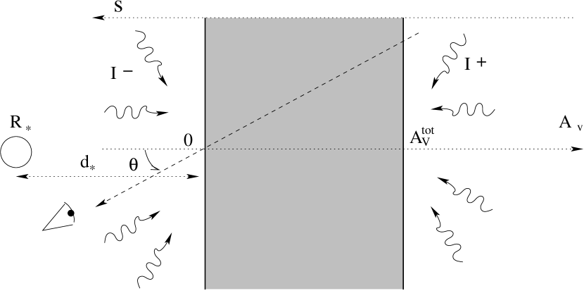
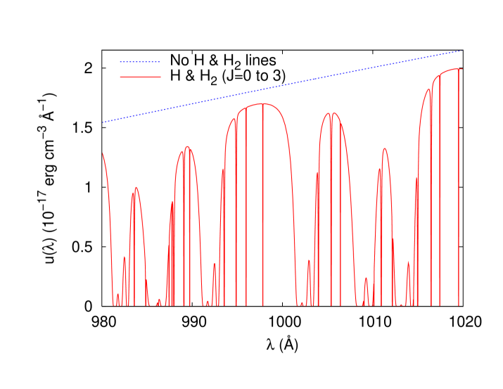
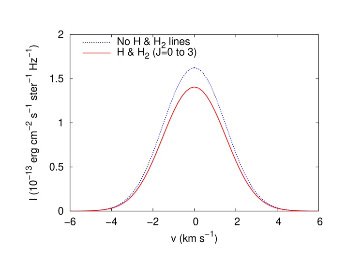
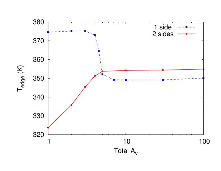
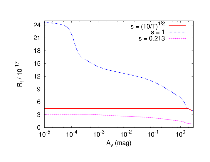
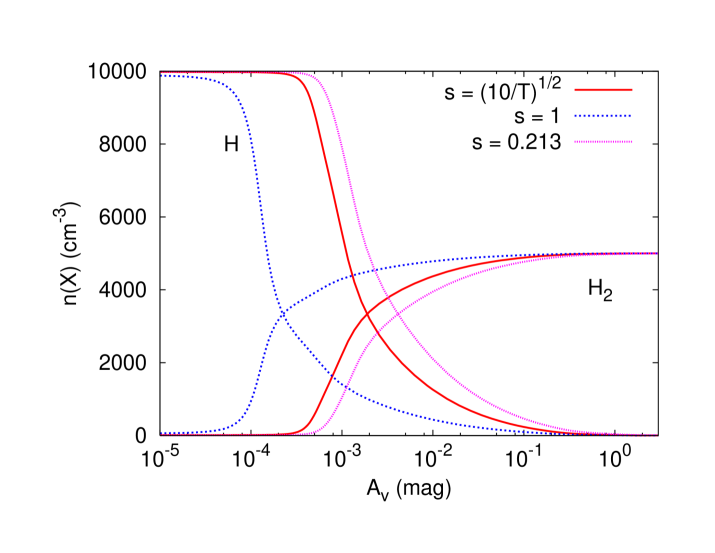
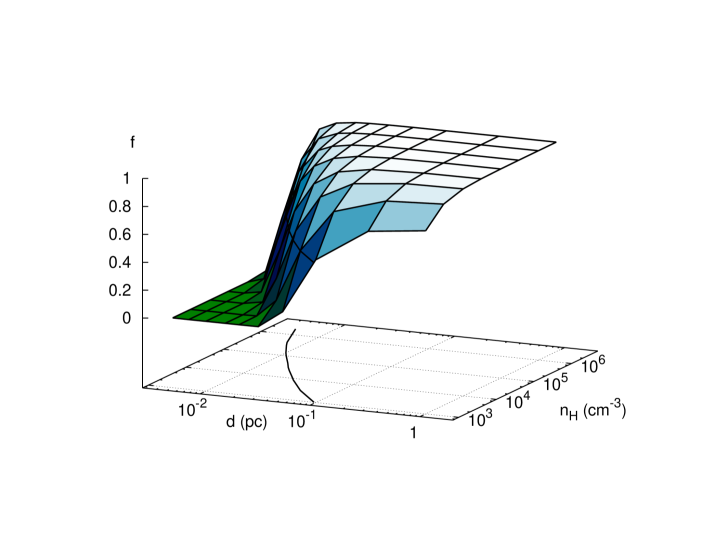
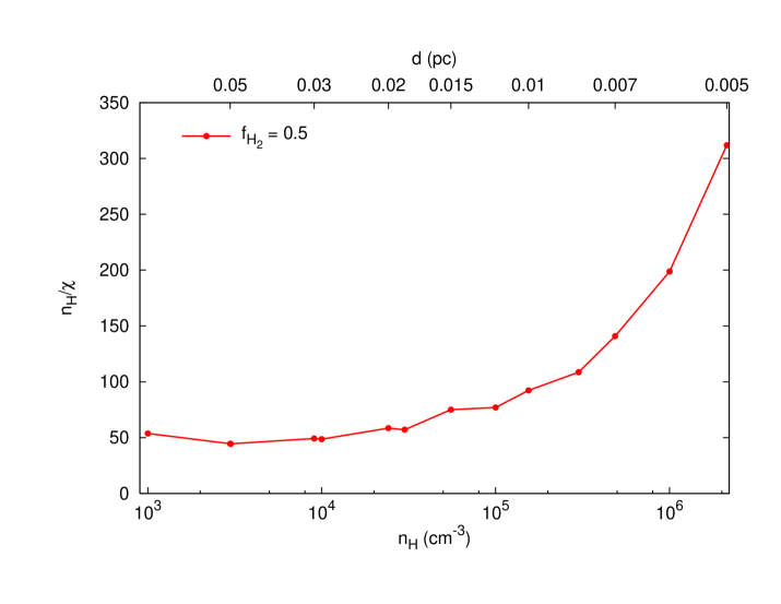
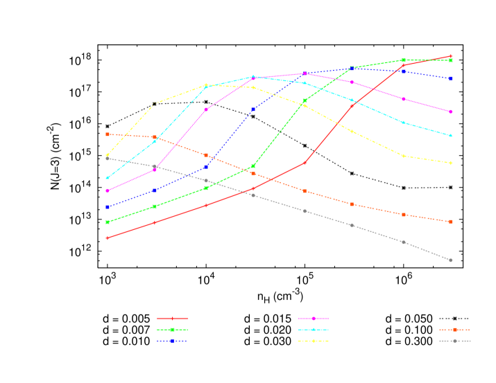
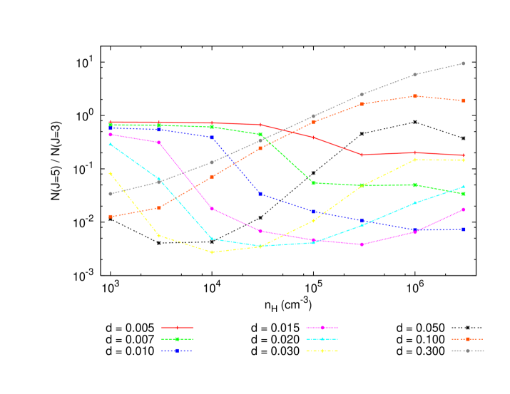
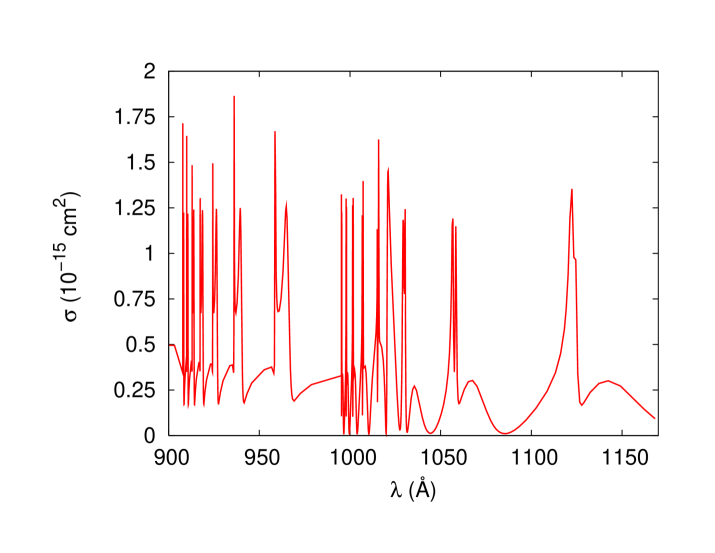
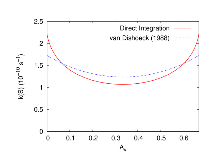
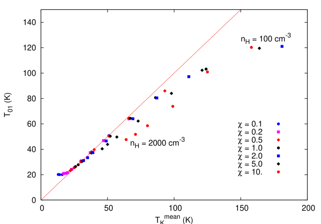
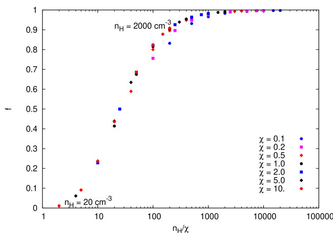
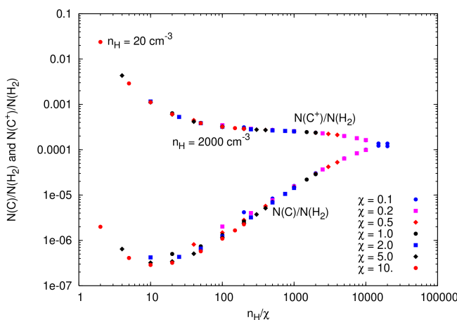
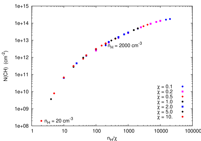
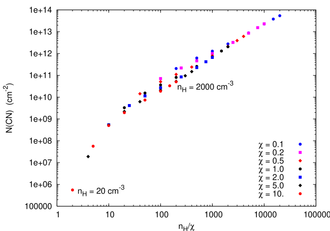
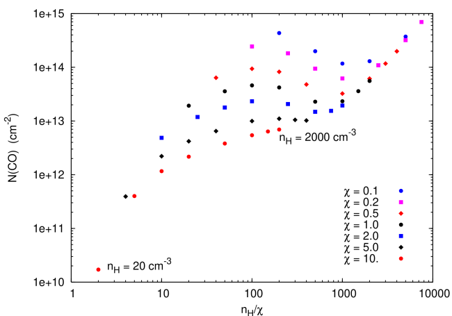
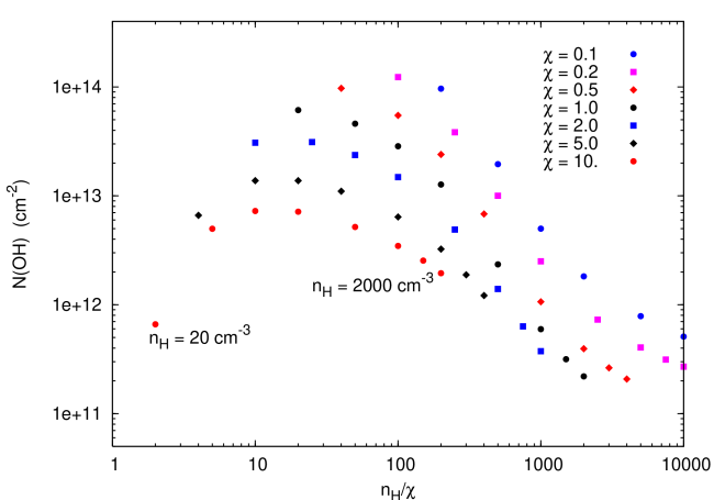
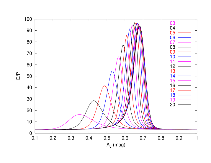