An ultradeep submillimetre map: beneath the SCUBA confusion limit with lensing and robust source extraction

Abstract

Extracting sources with low signal-to-noise from maps with structured background is a non-trivial task which has become important in studying the faint end of the submillimetre number counts. In this article we study source extraction from submillimetre jiggle-maps from the Submillimetre Common-User Bolometer Array (SCUBA) using the Mexican Hat Wavelet (MHW), an isotropic wavelet technique. As a case study we use a large (11.8 arcmin²) jiggle-map of the galaxy cluster Abell 2218, with a 850-$\mu$m 1$\sigma$ r.m.s. sensitivity of 0.6-1 mJy. We show via simulations that MHW is a powerful tool for reliable extraction of low signal-to-noise sources from SCUBA jiggle-maps and nine sources are detected in the A2218 850-$\mu$m image. Three of these sources are identified as images of a single background source with an unlensed flux of 0.8 mJy. Further, two single-imaged sources also have unlensed fluxes $<2$ mJy, below the blank-field confusion limit. In this ultradeep map, the individual sources detected resolve nearly all of the extragalactic background light at 850 $\mu$m, and the deep data allow to put an upper limit of 44 sources per arcmin² to 0.2 mJy at 850 $\mu$m.

1 Introduction

The arrival of the Submillimetre Common-User Bolometer Array (SCUBA; Holland et al. 1999) on the James Clerk Maxwell Telescope (JCMT) heralded a new era in galaxy evolution studies. The populations of submillimetre-bright, high redshift galaxies (Smail et al., 1997a; Hughes et al., 1998; Barger et al., 1998) have been studied using three different observational strategies: gravitational lens surveys, where pointings are made in the regions of well known cluster lenses hence benefiting from the cluster magnification, blank field surveys, generally selected to overlap with areas already observed at other wavelengths, and pointed photometry of targets selected in other bands.

The blank field surveys (Barger et al. 1999; Hughes et al. 1998; Eales et al. 2000; Scott et al. 2002; Borys et al. 2003; Webb et al. 2003) have produced counts at fluxes brighter than $S_{850}\sim$ 2 mJy. This flux limit is caused by the source confusion, which for the 15^′′ angular resolution of the JCMT at 850 $\mu$m appears to become a problem at about 2 mJy, effectively limiting the depths of these surveys (Condon 1974; Blain et al. 1998; Barger et al. 1999; Eales et al. 2000; Hogg 2001). To this flux limit 35-45% (e.g., Borys et al. 2003) of the submillimetre extragalactic background light (Puget et al., 1996; Fixsen et al., 1998) is resolved.

In comparison, the cluster gravitational lens surveys (Smail et al. 1997a, 2002; Cowie et al. 2002; Chapman et al. 2002; Knudsen et al., in prep.), probe sources fainter than the blank field confusion limit. As the lensing transformation is a mapping from source plane to image plane, it changes the number density of observed sources: Both the flux of a given source and the area of the region surveyed are magnified. As a result the confusion limit is moved to a fainter flux level, thereby enabling us to reliably study the fainter sub-mm galaxy population, which would otherwise not be accessible with the current telescopes and instrumentation. The magnification can be very large near critical lines, where we expect to see multiple images of the background sources (Kneib et al., 1996). The typical size of the critical lines is 20-30″ in radius for massive clusters and hence SCUBA’s 2.3′ diameter field-of-view is very well-matched to the high magnification region of typical cluster lenses.

This faint population, which can currently only be probed via lensing, is crucial to study as it is an important contributor to the extragalactic submillimetre background light (e.g., Blain 1997, 1999; Borys et al. 2003; Knudsen 2004). While many tens of submillimetre galaxies with fluxes $>$4 mJy have already been studied in great detail probing their redshift distribution, gas content etc. (e.g., Chapman et al. 2005; Greve et al. 2005), very little is known about the faint population as it yet has been possible only to identify and study a handful of objects in detail (e.g., Kneib et al. 2004a; Borys et al. 2004).

In this paper we present one of the deepest ever SCUBA maps of a massive galaxy cluster: Abell 2218, a rich galaxy cluster at redshift $z=0.175$ (Abell et al., 1989) and acts as a powerful gravitational lens both distorting and magnifying the distant galaxies (Kneib et al., 1996). It has already proven to be a powerful tool in studying high redshift, faint galaxies. Exploiting the gravitational lensing, several background galaxies have been found, including the lensed $z=5.57$ galaxy of Ellis et al. (2001). Probably the most unusual galaxies have been a multiply-imaged submillimetre galaxy seen as three distinct images (Kneib et al., 2004a), which have already been studied in great detail at other wavelengths (Kneib et al., 2005; Sheth et al., 2004; Garrett et al., 2005), and a redshift $z\sim 7$ galaxy (Kneib et al., 2004b; Egami et al., 2005).

To analyse this new SCUBA map, we used a novel technique based on the Mexican Hat Wavelet (MHW, so-called because the mother wavelet is like a sombrero in 3-d space) technique and routines developed by Cayón et al. (2000), Vielva et al. (2001a, b) and Vielva (2003) for use with anticipated Planck Surveyor data. In the analysis of the Planck data MHW will be used for removing contaminating foreground extragalactic point sources and leave the Cosmic Microwave Background (CMB) signal. However, in this paper we are interested in the point sources themselves as the end product. The key advantage of the MHW technique is that without needing to characterise the background and noise in an image, Gaussian shaped beams can be picked out from a variety of backgrounds with accurate positions and fluxes. This makes the technique ideal for submillimetre images where sources are significant in size with respect to the field-of-view, and the noise is often relatively high, variable across the field and hard to model accurately. Barnard et al. (2004) successfully applied MHW as a source extraction tool on SCUBA scan-maps of Galactic regions and placed valuable upper limits for the source counts of submillimetre galaxies at 50 and 100 mJy.

This paper is Paper I in a series of two papers and is an introduction to the use of the MHW technique in SCUBA jiggle-maps followed by its application on the deep Abell 2218 SCUBA map. The SCUBA data presented here include more observations than were published for the same cluster in Kneib et al. (2004a). Paper II (Knudsen et al., in preparation) presents the multi-wavelength identification of the underlying galaxies giving rise to the submillimetre emission. The present paper is organized as follows: Section 2 covers the observations and the data reduction. In Section 3 we discuss in details the MHW technique. The detailed analysis of the Abell 2218 sub-mm maps, the detected sources and derived number counts are discussed in section 4. Conclusions and prospects are summarised in section 5. In a further paper (Knudsen et al., in prep.) we will describe the results of applying the MHW technique to a wider survey of cluster lenses (the Leiden-SCUBA Lens Survey).

Throughout we will assume an $\Omega=0.3$, $\Lambda=0.7$ cosmology with $H_{0}=70$ km s^-1 Mpc^-1.

2 Observations and data reduction

2.1 Observations

We obtained observations of the cluster of galaxies A2218 at 850 $\mu$m and 450 $\mu$m with SCUBA during March 1998, August 2000, January 2001 and January 2002. SCUBA is a submillimetre mapping instrument operating at 850 $\mu$m and 450 $\mu$m simultaneously (Holland et al. 1999). SCUBA consists of two arrays of bolometers having 37 elements at 850 $\mu$m and 91 elements at 450 $\mu$m. The field–of–view on the sky, which is approximately the same for both arrays, is roughly circular with a diameter of 2.3′. The observations were carried out in jiggle mode, where the secondary mirror follows a 64-point jiggle pattern in order to fully sample the beam at both operating wavelengths. In order to cover a larger sky area four pointings were made, though with a big overlap region. As the region with large gravitational lensing magnification is extended due to the double-peaked mass distribution of A2218, four pointings were obtained. The offsets between the central position of each pointing were about 0.5 arcmin. The primary sky subtraction is achieved by chopping the secondary mirror. The chop configuration used for most of the time was a chop throw of 35″ with a position angle fixed in right ascension (RA), though larger chop throws and other position angles were also used for a limited part of the observations. The resulting beam, weighted by time spent using the different chop throws, is shown in Figure 1. As a result of chopping to either side the beam pattern has a central positive peak with a negative dip on each side in the chop direction with amplitudes of half the peak flux.

During the observations the pointing was checked every hour by observing nearby bright blazars with known positions. The noise level of the bolometer arrays was checked at least twice during an observing shift, and the atmospheric opacities at 850 $\mu$m and 450 $\mu$m, $\tau_{850\mu{\rm m}}$and $\tau_{450\mu{\rm m}}$, were determined by a JCMT skydip observation every two–three hours and supplemented with the $\tau_{225{\rm GHz}}$ data from the neighboring Caltech Submillimeter Observatory (CSO). The zenith opacity was 0.15 $<\tau_{850\mu{\rm m}}<$ 0.40 (corresponding to 0.037 $<\tau_{225{\rm GHz}}<$ 0.1), although data taken when $\tau_{850\mu{\rm m}}>$ 0.32 were not included in the 450-$\mu{\rm{m}}$ map since it is much more sensitive to poor weather. Calibrators with accurately known flux densities were observed every two to three hours. If available, primary calibrators, i.e. planets, preferably compact Uranus, were observed at least once during an observing shift. The uncertainty in the flux calibration is approximately 10 % at 850 $\mu$m and approximately 30 % at 450 $\mu$m.

The on-sky exposure time was 39.7 hours at 850 $\mu$m and 33.4 hours at 450 $\mu$m without overhead, i.e. without time needed for the chopping, jiggle, etc. The total area surveyed is 11.8 arcmin² at 850 $\mu$m and 9.1 arcmin² at 450 $\mu$m.

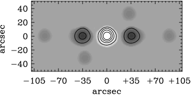
Figure 1: The 850 $\mu$m beam map. The contours represent the levels $-$0.3 to 0.9 in steps of 0.2. The data for A2218 were obtained with different chopping configurations. The beam map was constructed by weighting the different chop configurations with observing time. Most of the data were obtained with a chop throw of 35″. The configurations with chop throws of 45″ and 90″ were used for a short time in the observations, which is reflected by the few per cent in the beam map. The negative dips at 35″ have a little tail away from the central peak, which is due to the 45″ chop throw.

Figure 2: In this mosaic the SCUBA flux maps (top) of A2218 and the corresponding noise maps are shown (bottom). The left side represent the 850 $\mu$m maps, and the right side the 450 $\mu$m maps. Top-left: The 850 $\mu$m flux map overlaid with 850 $\mu$m signal-to-noise contours of $S/N=\,$3,4,5,6,8,12,18,24. The map has been cleaned and sources have been restored using the central positive peak of the beam (see Sect. 2.4). The map has been smoothed with a two-dimensional Gaussian with width 5″. The white line indicate the area being used in the further analysis. Top-right: The 450 $\mu$m flux map overlaid with the 450 $\mu$m signal-to-noise contours of $S/N=\,$3,4,5,7,10. The map has been smoothed with a two-dimensional Gaussian with width 10″. Bottom-left: The 850 $\mu$m noise map. This map represents the position dependent noise after smoothing with 5″. The contours have been overlaid to enhance the contrast and are 0.8 to 3.6 mJy/beam in steps of 0.4 mJy/beam. Darker shades of grey indicate a lower noise. The dashed line indicates the area of the map. The edges are clearly less sensitive and the whole edge region of the map is not included in the analysis. The white line indicate the area being used in the further analysis. Bottom-right: The 450 $\mu$m noise map. This is the noise map for the data smoothed with 10″. The contours have been overlaid to enhance the contrast and represent 4 to 16 mJy/beam in steps of 2 mJy/beam. The dashed line indicates the area of the map. Comparing left to right, the slightly smaller field of view at 450 $\mu$m is evident.

2.2 Reduction

The data were reduced using the standard surf package (Jenness & Lightfoot 1998). The reduction procedure is described in detail in the catalogue paper for the Leiden-SCUBA Lens Survey (Knudsen, 2004). The maps have been regridded with a pixel scale of $1^{\prime\prime}$. The full width at half maximum (FWHM) of the beam is 14.3″ in the final 850 $\mu$m and 7.5″ in the 450 $\mu$m.

Only the beam scale and above is real information reflected. Thus to suppress artificial pixel noise, the maps are smoothed to reduce the spatial high frequency noise. The 850 $\mu$m and the 450 $\mu$m maps were smoothed using a 2-D Gaussian function with a FWHM of 5″ , yielding the beams of 15.1″ and 9″ respectively. Additionally, to match the beamsize of the 850 $\mu$m, the 450 $\mu$m map is smoothed with a 2-D Gaussian with FWHM of 10″ , which results in a beam of 12.5″ , comparable to the beam size at 850 $\mu$m. The resulting maps are shown in Figure 2. The sensitivity in the final 850 $\mu$m map is 0.65 mJy/beam in the deepest part of the map and 1.1 mJy/beam averaged across the map. This is of equivalent depth to the 850-maps published by Cowie et al. (2002). The sensitivity in the final 450 $\mu$m map is 4.3 mJy/beam in the deepest part and 14 mJy/beam averaged across the map, as determined from the noise simulations described below.

In this paper we concentrate on the 850 $\mu$m map. In general the analysis of 450 $\mu$m maps is more difficult because the 450 $\mu$m beam pattern is very sensitive to temperature variations on the primary mirror of the JCMT. The beam pattern cannot easily be described by a 2D Gaussian function. Furthermore, both the atmospheric opacity and the uncertainty in the flux calibration are large at 450 $\mu$m. This makes observations of faint objects difficult. However, given the good quality of the 450 $\mu$m data obtained for A2218 we do include the 450 $\mu$m flux for the 850 $\mu$m sources (Table 2).

2.3 Construction of noise maps

When a data set is combined and regridded into a map, some areas are sampled less than the rest of the map. In the A2218 images, these include the areas along the edges, the areas where the bolometers are either more noisy or where data has been excluded, and areas with less integration time outside the overlap between different pointings. It is thus imperative to assess the noise as function of position in the map to be able to make a reliable analysis of the observed flux map.

When data files for the SCUBA jiggle maps have been fully reduced, i.e. all correlated noise has been removed, the noise in each individual bolometer can be assumed to be independent of other bolometers. The sources we are observing are very faint and thus large integration times are necessary in order to reach the needed noise levels for detections. However, the observations are carried out on short time scales on the order of an hour, which are the standard lengths of our observations, thus the data stream from the bolometers are dominated by noise rather than signal.

In order to determine the position–dependent noise a Monte Carlo simulation was used to construct ‘empty’ (i.e. no source signal present) maps representing the noise component in the real data files. For each original data file, the statistical properties of each bolometer’s data set were calculated. Then a simulated data set for each bolometer was created using a Gaussian random number generator with the same properties. This produced an empty map for each original data file, and the entire set of these was reduced and concatenated using surf in the same manner as the original data files. The resultant single map is thus one realization of the empty map simulation procedure. This process was then repeated about 500 times. Noise maps were constructed from the simulated empty maps by taking all the empty maps and calculating the standard deviation at each pixel. The noise maps at both 850 $\mu$m and 450 $\mu$m are shown in Fig. 2, where it can be seen how the noise is not uniform across the field and how the different effects described above appear.

This algorithm is similar to looking at the scatter of the data that goes into each pixel. It does not take into account residual 1/f noise and other systematic errors. Comparing the two methods suggests the difference is only at the 10% level (C. Borys, private communication).

2.4 Deconvolution of beam map

As described in section 2.1, the chopping of the secondary mirror on either side of the central pointing creates a beam pattern with a positive peak and two negative sidelobes. This is undesirable because negative sidelobes can hide sources or bias their fluxes. Also the negative sidelobes contain useful signal that can be used in source detection. Therefore it is useful to deconvolve the beam pattern out. Since we are dealing mostly with isolated point sources the classical CLEAN algorithm (Högbom 1974) is ideally suited for this purpose. In summary, the classical CLEAN algorithm is an iterative algorithm which searches for the brightest point, which matches the beam pattern, in the final map. The beam pattern is scaled to some fraction of the peak flux and subtracted from the map at that position. The whole process is then repeated in principle until the residual map has an r.m.s. comparable with the noise, though in practice until a given flux limit. All the information about subtracted fluxes and positions (the resultant “delta-functions”) can then be used for source detection and restoration with a different beam pattern e.g. the central positive peak of the beam pattern.

In our cleaning algorithm, the (cleaned) data map was convolved during each iteration with the beam map and divided by the associated convolved noise map. The former step enhances any present signal in the map whilst the latter ensures that no noise peaks (e.g. along the edges) would be mistaken for signal. This image is then used to select the peaks, but the cleaning itself takes place on the unconvolved data map. We found that subtracting 10 % of the flux at each iteration produced acceptable convergence. The cleaning was continued until the residual map contained no pixels brighter than three times the r.m.s. noise level. Finally, the detected sources were convolved with the positive peak of the beam map and coadded to the uncleaned residuals to give a final cleaned map. Using the central positive peak to restore the sources in the map preserves the information about the beam shape, which will be important for the source extraction. The cleaned 850 $\mu$m map, where the sources have been restored using the central positive peak of the beam, is shown in Figure 2. The 450 $\mu$m map has been cleaned in the same manner and is also shown in 2.

3 Mexican Hat Wavelet Source Detection

Independent of the survey strategy, the source extraction algorithm applied to the SCUBA maps must be a robust, well-characterized method. Indeed, the noise in SCUBA jiggle maps has a temporal variation and the sources we wish to detect typically have at best moderate signal-to-noise ratio ($S/N$). The far-infrared emitting regions in high redshift sources are expected to be relatively compact and so are likely to be unresolved in SCUBA’s 15″ beam. While Mexican Hat Wavelet source detection is the scope of this paper, we first summarise a number of techniques have been used for locating point sources in previous SCUBA jiggle-maps.

In the cluster lens surveys, extraction techniques have tended to be simpler, as these surveys cover smaller fields with fewer sources. Smail et al. (1997a) and Smail et al. (2002) used SExtractor (Bertin & Arnouts 1996), which was primarily developed for use in optical images which have very different noise characteristics to SCUBA maps. In the Hawaiian deep fields, Barger et al. (1999) simply used a signal-to-noise criterion for their source selection, a technique also used for the HDF (Hughes et al., 1998).

For the ongoing SCUBA Half-Degree Extragalactic Survey (SHADES) a matched-filter source-extraction technique has been demonstrated for a sub-set of data (Mortier et al., 2005).

In their jiggle-maps of the Canada UK Deep SCUBA Survey (CUDSS) fields, Eales et al. (2000) and Webb et al. (2003) selected sources from a convolved signal-to-noise map, which was constructed by convolving their reduced map with a beam map derived from a calibrator, and dividing by a simulated noise map (see section 2.3). An iterative deconvolution (CLEANing) routine was then used for determination of the position and flux of the detected sources.

In the 8-mJy survey (Scott et al. 2002), sources were extracted by a simultaneous maximum-likelihood fit to the flux densities of all probable peak locations, selected purely on the grounds of flux. A template beam map from a calibration observation was centred on every pixel with flux $>\,$3 mJy in a map convolved with a Gaussian filter. The height of each potential source was then increased independently until a minimum was found in the $\chi^{2}$ statistic between this built-up map and the real map. A similar approach was used in the extended Hubble Deep Field (HDF) and flanking fields source extraction (Serjeant et al. 2003). In short, in the two methods applied to the CUDSS and to the 8-mJy survey data sets the images are convolved with the beam. The methods differ in how the convolved images are converted to a catalogue.

3.1 MHW Detection parameters

The standard mathematics and detection parameters involved in the Mexican Hat Wavelet (MHW) transform were given in Barnard et al. (2004). Further details can also be found in the original papers describing this work (Cayón et al. 2000; Vielva et al. 2001a, b).

Point source detection is primarily controlled by setting numerical requirements for two parameters, namely an optimal scale, $R_{opt}$, and an wavelet coefficient value, $w_{f}(R_{opt})$. We performed initial, simple simulations, using both real data and the simulated noise maps from the previous section, to understand the response of the MHW routines to SCUBA jiggle-maps, since these are quite different in several respects to the simulated $Planck$ data sets on which the technique was previously tested. The procedure involved in selecting sources for the final detection list is as follows:

1. Firstly the optimal scale, $R_{opt}$, is calculated by the MHW software for each input map. This involves iterating through small changes in the value of $R$ around the point source scale, $\theta$, until the maximum amplification is found for the map. The final value will be dependent upon the measured impact of the noise on varying scales (Vielva et al. 2001b) — noise with a characteristic scale a little larger than $\theta$, for instance, can be most strongly counteracted by an optimal scale $R_{\rm{opt}}$ slightly smaller than $\theta$.

2. Point source candidates are then selected at positions with wavelet coefficient values $w_{f}(R_{opt})\geq 2\sigma_{w_{n}}(R_{opt})$, where $\sigma_{w_{n}}(R_{opt})$, where $\sigma_{w_{n}}(R)$ is the dispersion of the noise field in wavelet space. The value of 2 was suggested by our early simulations as a value which allowed all real sources to pass through to an initial catalogue.

3. For each candidate, the ‘experimental’ $w_{f}(R)$ is compared to the theoretical variation expected with $R$, as a further check on the source’s shape. A value of $\chi^{2}$ is calculated between the expected and experimental results and the second parametrised requirement is therefore that $\chi^{2}\leq 4$, i.e. that the region surrounding the identified peak has the characteristics of a Gaussian point source.

Since, as discussed in Section 2.3, the noise level in the map varies widely, the input map to the MHW software used was a signal-to-noise map, created by dividing the final, smoothed data map by the final, smoothed noise map. This normalises the input map with respect to the noise. This is especially useful for this technique as the properties of the whole map are used to determine detection parameters, and so high noise values can distort these values unfairly.

Despite this normalisation, detections close to the edge of the map, where the noise levels are at their highest, were considered to still be unreliable and such detections in a 1.5-beam region around the edge are not retained in the final catalogue. As discussed in previous papers (e.g., Ivison et al. 2002) the number of spurious detections in SCUBA maps is larger along the edges than elsewhere in the maps.

To assess the chances of obtaining false positive detections in the $S/N$ map, we performed the MHW source extraction upon empty $S/N$ maps, created by dividing the empty Monte Carlo maps by the final average noise map. In 100 such realisations we found only two sources with $S/N>$ 3. We thus conclude that, when restricting the sources to those which both meet the standard detection parameter requirements outlined and which have $S/N>$ 3 in real space, the probabililty of spurious detections is very low. A detailed analysis of this is performed for the full Leiden-SCUBA Lens Survey (Knudsen, 2004; Knudsen et al., in prep.).

Table 1: MHW and CLEAN detections

	MHW						CLEAN
	uncleaned			cleaned
src	$\Delta x$	$\Delta y$	$f$	$\Delta x$	$\Delta y$	$f$	$\Delta x$	$\Delta y$	$f$
1	78	-40	10.8	79	-40	10.4	78	-41	9.0
2	20	-17	9.0	20	-17	8.7	18	-17	9.2
3	-1	2	17.1	-0	1	16.1	-1	0	22.3
4	-6	15	11.7	-6	14	12.8	-8	14	11.3
5	-6	-34	5.0	-6	-34	3.1	-7	-34	3.2
6	-8	36	11.0	-8	36	11.3	-11	36	13.9
7	-54	30	4.3	-51	31	3.3	…	…	…
8	-69	35	5.4	-69	35	5.2	-68	32	3.8
9	-75	10	4.6	-74	10	4.8	-75	10	4.4
10	45	13	4.4	…	…	…	…	…	…
11	59	-17	4.0	…	…	…	…	…	…
12	113	-1	9.3	…	…	…	…	…	…
13	…	…	….	…	…	…	-30	68	2.0
14	…	…	….	…	…	…	-10	69	2.3
15	…	…	….	…	…	…	2	29	2.4
16	…	…	….	…	…	…	30	50	2.6

Note:   $\Delta x$ and $\Delta y$ give the distance in pixels from the map centre at $\alpha,\delta$ = 16^h35^m54.22^s,+66^∘12′24″, and the pixel scale is 1 arcsec/pixel. The flux, $f$, is in units mJy.

3.2 Comparison of MHW and CLEAN source detection

We compare the MHW source detection done on the un-cleaned map and the cleaned map. x,y pixel positions relative to the centre of the map and fluxes for detections are listed in Table 1. The first nine sources are numbered according to their number in the final catalogue as given in Table 2. The positions agree very well for all nine sources, though for source 7 there has been a four pixel shift. Source 7 is close to the negative sidelopes of the bright central sources. In the cleaned map its wavelets parameters are much improved and its profile provides a better match to the theoretical expectation as estimated by the MHW algorithm. Source 7 is the reason why we CLEANed the SCUBA map for this project, i.e., to confirm whether the source was an artifact due to the negative sidelopes of the beam. For the other sources the wavelets parameters were improved only by a few percent when using the cleaned map. In the uncleaned map three additional sources were detected. Source 12 falls within the edge region, which has been trimmed off. Sources 10 and 11 do not produce a good match to the theoretical wavelets expectation. As these sources were not re-detected in the cleaned map, we consider them spurious.

Furthermore, we compare the MHW source detections with the detections from the CLEAN algorithm (also shown in Table 1). The CLEAN algorithm detects twelve sources, of which eight are in good agreement with those detected by the MHW algorithm. CLEAN yields larger flux estimates for sources 3 and 6. The positions deviate by about 1-2 pixels from the MHW position, but in general there is good agreement between the two methods. Source 7 is not detected by CLEAN. The four additional sources (13-16) are faint, $\sim$ 2 mJy, and remain undetected by MHW. The reason for this could be found in how the two methods depend on the zero-point of the map: If large scale variations across the map elevate the zero-point of the map, this will also have an impact on the $S/N$ value so that these appear systematically off-set by a small value. For the CLEAN routine, which selects the sources by $S/N>3$, also positions with artificially increased $S/N$ ratio will be selected. The MHW algorithm, which searches for sources of a given scale placed on top of a background, such large scale variations will have no or only very small influence on the detection of sources, and thus MHW remains essentially insensitive to the zero-point of the map. For future large surveys, such as those planned to be carried out with SCUBA-2, large scale variations can pose a problem. MHW may offer a good solution for source extraction from such maps.

Finally, in order to check the MHW source detection, in order to check for possible sources hidden in the wings of bright sources, we subtracted the detected sources from the map, using a template for the central beam scaled to the fluxes of the individual sources. This residual map is not the residual map from the CLEAN routine, as it still contains the sources which were detected by CLEAN but not by MHW. Then, we performed source extraction with MHW on the residual image. If there is a source closer than a beam to the other sources, which has remained undetected, then we expect to detect it in the residual map. Four such sources are detected. Three of these are directly associated with bright sources and are likely artifacts resulting from an imperfect match of the bright source and the scaled beam subtracted from the map. The fourth source may be real, but is outside of the 7.7 arcmin² trimmed region near the SW edge and thus no included in the analysis. So in conclusion we believe that our MHW catalogue is robust and does not miss any sources to the detection limit of the data.

3.3 Testing MHW with simulations

Figure 3: Upper panels:  The relative difference between the input and detected flux as function of $S/N$ (left) and flux (right) based on the simulations. The filled dots represent the average in each $S/N$ or flux bin, while the error bars represent the standard deviation in the same bin. Lower left panel:  The standard deviation ($\bullet$) of the difference between input and detection position as a function of $S/N$ based on the simulations. Lower right panel:  The completeness as function of input flux based on the simulations. The 850 $\mu$m map is 80 % complete at 3.8 mJy and 50 % complete at 2.7 mJy. For comparison, 3 mJy corresponds to $S/N\sim 3$ in about two-thirds of the map.

Using the empty Monte Carlo maps we investigated the detection accuracy of the MHW algorithm in a similar fashion as was performed for the scan-maps in Barnard et al. (2004). One point source was added at a time to the empty maps using the central peak of the beam map shown in Figure 1 as a template source. This was repeated 400 times for each flux step. The position was randomly chosen, with a uniform distribution across ten maps, so that the whole map area was well sampled. The input flux of the point source was then increased and the standard MHW detection algorithm was run on each map. Additionally, we also perform two simulations for the CLEAN routine concerning sources close to the edge and overlapping sources.

3.3.1 Position accuracy

In Figure 3 we plot the standard deviation of the difference between input and detection position. The standard deviation decreases with increasing $S/N$ and has a value about 2.5″ at $S/N\sim$ 3 decreasing towards 0.5″ for large $S/N$. We adopt these as the uncertainty on the determined position introduced by the extraction algorithm. This added in quadrature with the pointing uncertainty of the JCMT ($\sim$2″) gives the error on the determined position.

3.3.2 Flux accuracy

In Figure 3 we plot the relative average flux difference, $(S_{out}-S_{in})/S_{in}$, and the standard deviation as function of $S/N$ and of flux. For $S/N>7$ and also flux $>$ 7 mJy the detected flux on average is overestimated by one to two percent. Eddington bias is seen through the average overestimation of the sources with fainter fluxes and lower $S/N$. This is also seen in other SCUBA surveys (e.g., Scott et al. 2002; Webb et al. 2003; Borys et al. 2003; Barnard et al. 2004). We note that the calibration uncertainty is larger than the Eddington bias. The standard deviation on the average relative flux difference decreases with $S/N$, from about 25% at $S/N=3$ to 5-7% at $S/N>15$. As uncertainty on the determined flux we use the standard deviation of the relative average flux different, which is added in quadrature with the calibration error from the SCUBA reduction to give the total error on flux density of the individual sources.

3.3.3 Completeness

The completeness as function of input flux was determined from the same set of simulations. The fraction of sources detected at each flux level is calculated. The result is plotted in Figure 3. The observations are 80 % complete at 3.8 mJy and 50 % complete at 2.7 mJy.

3.3.4 Sources near the edge

For sources closer to the edge one of the two negative sidelopes will be outside of the map. This can complicate the source detection in CLEAN, where a matching to the full beam pattern is done. In simulating 400 point sources, one at a time, each of 20 mJy, we found that 68 sources, i.e. 17%, were not detected, while similar sources away from the edge were all detected. Additionally, the position and flux had larger uncertainties compared to those away from the edge.

3.3.5 Overlapping sources

Given the large width of the 850 $\mu$m beam, blending of sources is not an uncommon occurance. For example in the A2218 two of the nine sources are separated by approximately one beam width. We simulated source blending by adding two sources with a separation between 0 and 30 arcsec onto the MC maps. The flux ratio of the two sources was taken to be 1:1, 1:2 and 1:4, although we find that different flux ratios do not significantly alter the result in either case. MHW detects individual sources separated by more than one beam width, while CLEAN is able to detect sources with separations $>12\arcsec$. However, the flux and positions accuracies using MHW are on average approximately 5% better than those of CLEAN.

4 Analysis of Abell 2218 sub-mm maps

4.1 The sub-mm source catalogue

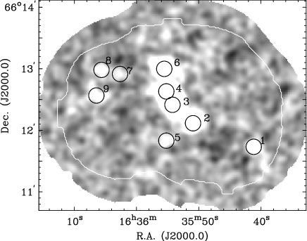
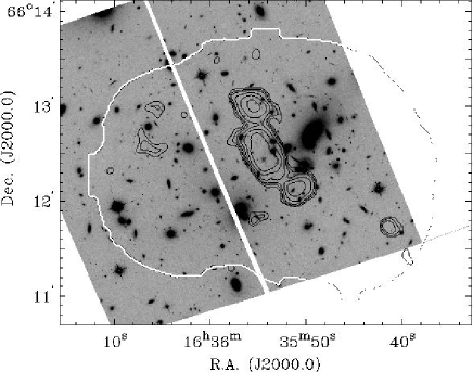
Figure 4: Upper panel:   A2218 850 $\mu$m $S/N$ map where the nine detected sources each are indicated with a circle with diameter of 15^′′. The number assigned to each source corresponds to their order in Table 2. The white line indicates the area used for the analysis. Lower panel:   The 850 $\mu$m $S/N=3,4,5,7,10,15$ contours overlaid on the HST ACS $z$-band image (Kneib et al., 2004b).

We now present the detailed analysis of the Abell 2218 SCUBA maps using the MHW technique. We focus on a total area of useful data of 7.7 arcmin² (see figure 2). Nine sources were detected by MHW using the detection parameters described in Section 3.1. Six of these sources have detectable 450 $\mu$m emission. The detected sources are listed in Table 2. The sources are named using the prefix SMM followed by their J2000 coordinates. For the 850 $\mu$m parameters we give the $S/N$ in real space, the combined flux and flux uncertainty and position uncertainty. For the 450 $\mu$m, where no emission is detected, we give 3$\sigma$ upper limits. The uncertainty on the 450 $\mu$m flux is 30%, which is derived from the calibration of the absolute flux. In Figure 4 we show the 850 $\mu$m $S/N$ map, and the $S/N$ contours overlaid on an optical image for orientation. The differences seen in flux, in particular at 450 $\mu$m, between these results and those of Kneib et al. (2004a) can be assigned to uncertainties in the calibration. More data has been included in the combined data set presented here than in the Kneib et al. (2004a).

Table 2: Sources detected in the SCUBA maps of A2218. $f$ is flux; $S/N$ is the signal-to-noise of the source in real space as detected using MHW; $\sigma$ gives the uncertainties on the flux and position at 850 $\mu$m and 450 $\mu$m respectively. The flux uncertainty is that found for the appropriate $S/N$ bin added in quadrature with the calibration uncertainty, as described in section 3.3.2. The positional uncertainty does not include confusion errors.

name		$\sigma_{pos}$	$f_{850}\pm\sigma_{850}$	$S/N$	$f_{450}\pm\sigma_{450}$	$S/N$	$z_{spec}$	$\mu$	$f_{850}/\mu$
		′′	mJy		mJy	mJy			mJy
SMM J163541.2$+$661144	(1)	2.9	10.4$\pm$1.4	7.5	$<59.4$	…	3.188	1.7	6.0
SMM J163550.9$+$661207⋆	(2)	2.7	8.7$\pm$1.1	11.5	39.2$\pm$11.8	7.2	2.516	45⋆	0.8
SMM J163554.2$+$661225⋆	(3)	2.6	16.1$\pm$1.6	21.7	89.7$\pm$26.9	19.0	2.516	45⋆	0.8
SMM J163555.2$+$661238⋆	(4)	2.6	12.8$\pm$1.5	16.9	60.1$\pm$18.3	12.1	2.516	45⋆	0.8
SMM J163555.2$+$661150	(5)	3.5	3.1$\pm$0.7	3.8	29.1$\pm$8.7	6.1	1.034	7.1	0.4
SMM J163555.5$+$661300	(6)	2.6	11.3$\pm$1.3	15.8	18.0$\pm$5.4	3.0	4.048	4.2	2.7
SMM J163602.6$+$661255	(7)	3.5	2.8$\pm$0.6	3.5	$<21.6$	…	…	1.8	1.6
SMM J163605.6$+$661259	(8)	3.3	5.2$\pm$0.9	4.9	$<25.5$	…	…	1.8	3.3
SMM J163606.5$+$661234	(9)	3.3	4.8$\pm$0.8	4.6	30.1$\pm$9.3	3.1	…	1.6	2.9

4.2 Gravitational Lensing Magnification

We exploit the detailed mass model of A2218 (Kneib et al., 1996) updated to include the triple sub-mm image (Kneib et al., 2004a) and the high redshift multiple images at $z=$ 5.56 (Ellis et al., 2001) and $z\sim 7$ (Kneib et al 2004b). In Figure 5 we show the area as function of magnification for source planes at the redshifts $z=$ 1 and 4. In 1.3 arcmin² the flux magnification factors are $>$ 2. Furthermore, in Figure 5 we show the area as function of sensitivity both in the image plane and in the source plane, again for source planes at different redshifts, $z=$ 1 and 4. For high redshift, $>1$, the lensing magnification is only weakly depending on redshift. For the sources without known redshift, assuming a redshift $>1$ will not have a strong impact on the derived properties. For $z>2$, the effective area surveyed (source plane) is about 2.7 arcmin² which corresponds to an average magnification factor of 2.8.

The redshift is known for six sources in the field: three of these are a multiply-imaged object at redshift $z=$ 2.516 (Kneib et al., 2004a), while the other three are single-imaged sources at redshift $z=$ 1.034 (Pelló et al., 1992), and $z=3.188$ and 4.048 (Paper II). For the sources with unknown redshift we assume $z=$ 2.5, based on the median redshift for bright SCUBA sources determined by Chapman et al. (2003, 2005). The magnification factors of the individual singly lensed sources range between 1.6 and 7.1. For the multiply-imaged source at $z=$ 2.516 the magnification factors for individual images are 9, 14 and 22, i.e. a total magnification of 45 for the three images combined (Kneib et al., 2004). In Table 2 we list the magnification factors, $\mu$, and the lensing corrected fluxes, $f_{850}/\mu$ for the individual galaxies.

Note that three (five, including all images of SMM J16359+6612) of the nine detected sources have unlensed fluxes fainter than or close to the blank field confusion limit. These sources would most likely not be detected in blank field surveys and thus not have been accessible to us without the use of gravitational lensing or a larger telescope with sensitive instruments.

Figure 5: Upper panel:   The area of the source plane as function of magnification for redshifts $z=1$ (dashed) and $z=4$ (dash-dot). The difference between the different redshifts is relatively small. Middle panel:   The area of the source plane as function of 3$\sigma$ sensitivity for redshifts $z=1$ (dashed) and $z=4$ (dash-dot). The source plane at $z=2.5$ is about 2.8 times smaller than the observed area of the image plane. Lower panel:   The confusion flux limit as function of magnification, as described in subsection 4.3.

4.3 Confusion

Confusion noise is caused by unresolved faint sources in the field. In the background of deep SCUBA maps the instrumental noise and the confusion noise from a fainter submm population are of approximately equal magnitude. Understanding the confusion in a map is essential to be able to estimate the relative importance of uncertainties due to blending of sources.

For the cluster fields the confusion limit is affected by the gravitational lensing. The gravitational lensing magnifies the region seen behind the cluster, hence the source plane is smaller than the image plane. The number of beams is conserved between the image plane and the source plane, i.e. the size of the beam scales with the magnification. This is why it is at all possible to observe the fainter sources, which have a higher surface density than the brighter sources.

The number counts in the lensed case can be written as $N_{lens}=(N_{0}/\mu)(S/\mu)^{-\alpha}$ $=N_{blank}\mu^{\alpha-1}$, where $\mu$ is the gravitational lensing magnification, assuming a blank-field number count power law where $N(>S)=N_{0}S^{-\alpha}$ and $S$ is the observed flux. The average magnification for a field can be found as the ratio of the area in the image plane and the area in the source plane. We use the rule of thumb, that the confusion limit in imaging is defined as one source per 30 beams (e.g. Hogg 2001). The confusion limit in the lensed case can thus be written as $S_{conf}=(30\Omega N_{0}\mu^{1-\alpha})^{1/\alpha}$ (illustrated in Figure 5), where $\Omega$ is the solid angle of the beam. As the lensing magnification varies across the field, this means that the actual confusion limit is deeper in highly magnified regions close to the caustics than the estimated average lensed confusion limit.

In case of the A2218 850 $\mu$m map, the confusion limit in the source plane based on this simple estimate is $\sim$ 1.1 mJy on average across the whole field. In the simplified estimate of the confusion limit presented here we assumed that the number counts are described by a single power law. There are good indications that the number counts are described by a double power law or another function with a (gradual) turn-over (Scott & White 1999; Scott et al. 2002; Borys et al. 2003; Knudsen 2004; Knudsen et al., in prep.). In the Leiden-SCUBA Lens Survey (Knudsen 2004), the 850 number counts are probed over almost two decades of flux (0.1-20 mJy) and improving the statistics in particular on the faint end. Including double power law number counts in such a calculation will work in a favourable direction and the confusion limit in the source plane will be lower.

4.4 850 $\mu$m source counts in A2218

In Fig. 6 we plot the number counts for sources detected in A2218. The number counts are calculated for the flux levels corresponding to the flux of each of the sources. Because of the large variation in the sensitivity across the map, it is not possible to directly determine the number counts as cumulative number counts. The complications arising from this has been discussed in previously (e.g., Borys et al. 2003; Webb et al. 2003). We here apply a simple method for estimating the number counts: At each flux level, $S$, only the area where $S>3\sigma$ are considered. The number of sources within that area are divived by the area. We use the sensitivity map for the source plane at redshift $z=2.5$ and note that using that of sources planes at other redshifts does not make a noticable difference. By using the source plane sensitivity map, we also take into account the effect that lensing has on the area. The error bars are Poisson statistics (Gehrels, 1986). The number counts are in reasonable agreement with the results from other surveys. Differences between surveys can be assigned to cosmic variance and small number statistics. The 850 $\mu$m number counts at the level of $\sim 1$ mJy is $\sim 2$ arcmin^-2. Additionally, we determine an upper limit for the number counts at $S_{850}=0.2$ mJy and 0.1 mJy of 44 arcmin^-2 and 175 arcmin^-2 respectively. The 450 $\mu$m number counts probe deeper than previously published Smail et al. (2002); Borys et al. (2003). They appear to be slightly higher, which can be assigned to sample variance, but agree within the error bars.

The fraction of the submm extragalactic background light (EBL) resolved in the SCUBA map can be constrained through the sum of the fluxes. The total flux relative to the area is (35$\pm$1.6) Jy deg^-2. This is $\sim$ 80% of the EBL as determined by Fixsen et al. (1998), and comparable to the EBL value determine by Puget et al. (1996). This almost double the total flux value of 17.3 Jy deg^-2 found by Cowie et al. (2002). Due to cosmic variance and the clustering of SCUBA sources, this value is expected to vary between fields. However, the fact that we resolve such a significant fraction of the EBL, is a good demonstration of the power of gravitational lensing in combination with the SCUBA observations, as it allows us to probe the faint submm galaxy population, which is the dominant contributor to the submm EBL.

5 Conclusions and outloook

We have performed a thorough analysis of the Mexican Hat Wavelet algorithm (MHW) as a source extraction tool applied to SCUBA jiggle-maps. The analysis was done using the deep SCUBA maps of the galaxy cluster A2218, through source extraction with MHW on the real data and through extensive simulations. We found that MHW is a stable method for source extraction at low signal-to-noise ($S/N>$ 3). We conclude that MHW is an algorithm suitable for source extraction from SCUBA jiggle maps and is a powerful tool for studying the faint submillimetre sources and thereby the faint end of the submillimetre number counts. MHW has potential as source extraction algorithm for data taken with the future SCUBA-2 instrument. SCUBA-2 will make “total power” maps, which should be free of chopping artifacts, hence MHW will have an immediate advantage over the other techniques currently in use.

The SCUBA map we have obtained for A2218 is one of the deepest submillimetre maps ever taken. Covering a large area of the cluster, we have been able to survey the region where strongly lensed background sources are present. In the analysis of A2218, nine sources were detected in the 850 $\mu$m SCUBA map, the largest number detected in a single ultra-deep SCUBA map. Six of these sources were also detected at 450 $\mu$m. Correcting for the gravitational lensing by the galaxy cluster, three sources have intrinsic 850 $\mu$m fluxes below the blank field confusion limit, and three with fluxes comparable to the blank field confusion limit. It is the presence of strong gravitational lensing, which pushes the confusion limit to fainter fluxes levels, which has made it possible to detect the faint submillimetre source with $<$ 2 mJy. For this field we determine the 850 $\mu$m number counts to $S_{850}=0.4$, and place upper limits at $S_{850}=0.1$ and 0.2 mJy. Additionally, we also estimate the 450 $\mu$m number counts down to $S_{450}=4$ mJy. The identification of the individual sources will follow in Paper II.

ALMA will in the future allow for yet deeper observations and thus a continuation of the number counts to even fainter fluxes. If ALMA will detect a number density of $\sim 50$ galaxies/arcmin², this means we are reaching the number density of galaxies detected in the optical/near-infrared and thus will allow for a better understanding of the connection between dust and stars in the Universe as function of time/redshift.

Figure 6: The 850 $\mu$m (left) and 450,$\mu$m (right) source counts in A2218 (filled circles). The upper limits for the very bright number counts from Barnard et al. 2004 are also shown (open circles). Furthermore, the number counts from four other surveys are included: the Lens SCUBA survey (diamonds; Smail et al. 2002), the 8mJy-survey (squares; Scott et al. 2002), the Canada-UK Deep SCUBA Survey (triangles; Webb et al. 2003) and the HDF Super-map (stars; Borys et al. 2003). The dotted line indicates the power-law counts used for calculating the confusion limit in subsection 4.3. The dashed line shows the blank field confusion limit. The vertical dash-dotted line indicate the 5$\sigma$ detection limit for a two hours observations with ALMA.

References

- (1)
- Abell et al. (1989) Abell, G.O., Corwin, H.G., Olowin, R.P., 1989, ApJS, 70, 1
- Barger et al. (1998) Barger, A.J., Cowie, L.L., Sanders, D.B., Fulton, E., Taniguchi, Y., Sato, Y., Kawara, K., Okuda, H., 1998, Nature, 394, 248
- Barger et al. (1999) Barger, A.J., Cowie, L.L., Sanders, D.B., 1999, ApJ, 518, L5
- Barnard et al. (2004) Barnard, V.E., Vielva, P., Pierce-Price, D.P.I., Blain, A.W., Barreiro, R.B., Richer, J.S., Qualtrough, C., 2004, MNRAS, 352, 961
- Bertin & Arnouts (1996) Bertin, E. & Arnouts, S., 1996, A&A, 117, 193
- Blain (1997) Blain, A.W., 1997, MNRAS, 290, 553
- Blain (1999) Blain, A.W., Kneib, J.-P., Ivison, R.J., Smail, I., 1999, ApJ, 512, L87
- Blain et al. (1998) Blain, A.W., Ivison, R.J., Smail, I., 1998, MNRAS, 269, L29
- Borys et al. (2003) Borys, C., Chapman, S., Halpern, M., Scott, D., 2003, MNRAS, 344, 385
- Borys et al. (2004) Borys, C., Chapman, S., Donahue, M., Fahlman, G., Halpern, M., Kneib, J.-P., Newbury, P., Scott, D., Smith, G.P., 2004, MNRAS, 352, 759
- Cayón et al. (2000) Cayón L., Sanz J.L., Barreiro R.B., Martínez-González E., Vielva P., Toffolatti L., Silk J., Diego J.M., Argüeso F., 2000, MNRAS, 315,757
- Chapman et al. (2002) Chapman, S.C., Scott, D., Borys C., Fahlman, G.G., 2002, MNRAS, 330, 92
- Chapman et al. (2003) Chapman, S.C., Blain, A.W., Ivison, R.J., Smail, I., 2003, Nature, 422, 695
- Chapman et al. (2005) Chapman, S.C., Blain, A.W., Smail, I., Ivison, R.J., 2005, ApJ, 622, 772
- Condon (1974) Condon, J.J., 1974, 188, 279
- Condon (1992) Condon, J.J., 1992, ARA&A, 30, 575
- Cowie et al. (2002) Cowie, L.L., Barger, A.J., Kneib, J.-P., 2002, AJ, 123, 2197
- Eales et al. (2000) Eales, S., Lilly, S., Webb, T., Dunne, L., Gear, W. Clements, D., Yun, M., 2000, AJ, 120, 2244
- Egami et al. (2005) Egami, E., et al., 2005, ApJ, 618, L5
- Ellis et al. (2001) Ellis R., Santos M., Kneib J.-P., Kuijken K., 2001, ApJ, 560, L119
- Fixsen et al. (1998) Fixsen, D.J., Dwek, E., Mather, J.C., Bennett, C.L., Shafer, R.A., 1998, ApJ, 508, 123
- Garrett et al. (2005) Garrett, M.A., Knudsen, K.K., van der Werf, P.P., 2005, A&A, 431, L21
- Gehrels (1986) Gehrels, N., 1986, ApJ, 303, 336
- Greve et al. (2005) Greve, T.R., et al., 2005, MNRAS, 359, 1165
- Hogg (2001) Hogg D.W., 2001, AJ, 121, 1207
- Holland et al. (1999) Holland, W.S., et al., 1999, MNRAS, 303, 659
- Hughes et al. (1998) Hughes, D.H., et al., 1998, Nature, 394, 241
- Högbom (1974) Högbom, J.A., 1974, A&AS, 15, 417
- Ivison et al. (2002) Ivison, R.J., et al., 2002, MNRAS, 337, 1
- Jenness et al. (1998) Jenness, T., Lightfoot, J.F., 1998, Astronomical Data Analysis Software and Systems VII , A.S.P. Conference Series, Vol. 145, 1998, R. Albrecht, R.N. Hook and H.A. Bushouse, eds.,p.216
- Kneib et al. (1996) Kneib J.-P., Ellis R., Smail I., Couch W., Sharples R., 1996, ApJ, 471, 643
- Kneib et al. (2004a) Kneib, J.-P., van der Werf, P.P., Knudsen, K.K., Smail, I., Blain, A.W., Frayer, D., Barnard, V., Ivison, R., 2004a, MNRAS, 349, 1211
- Kneib et al. (2004b) Kneib, J.-P., Ellis, R., Santos, M.R., Richard, J., 2004b, ApJ, 607, 697
- Kneib et al. (2005) Kneib, J.-P., Neri, R., Smail, I., Blain, A.W., Sheth, K., van der Werf, P., Knudsen, K.K., 2005, A&A, 434, 819
- Knudsen (2004) Knudsen, K.K., 2004, PhD. Thesis, Leiden University
- Mortier et al. (2005) Mortier, A.M.J., et al., 2005, MNRAS, 363, 563
- Pelló et al. (1992) Pelló, R., Le Borgne, J.F., Sanahuja, B., Mathez, G., Fort, B., 1992, A&A, 266, 6
- Puget et al. (1996) Puget, J.-L., Abergel, A., Bernard, J.-P., Boulanger, F., Burton, W.B., Desert, F.-X., Hartmann, D., 1996, A&A, 308, L5
- Sandell et al. (1994) Sandell, G., 1994, MNRAS, 271, 75
- Sanz et al. (2001) Sanz J., Herranz D., Martínez-González E., 2001, ApJ, 552, 484
- Scott & White (1999) Scott, D., White, M., 1999, A&A, 346, 1
- Scott et al. (2002) Scott, S.E., et al., 2002, MNRAS, 331, 817
- Serjeant et al. (2003) Serjeant S., et al., 2003, MNRAS, 344, 887
- Sheth et al. (2004) Sheth, K., Blain, A.W., Kneib, J.-P., Frayer, D.T., van der Werf., P., Knudsen, K.K., 2004, ApJL, 614, L5
- Smail et al. (1997a) Smail, I., Ivison, R.J., Blain, A.W., 1997a, ApJ, 490, L5
- Smail et al. (1997b) Smail, I., Ellis, R.S., Dressler, A., 1997b, ApJ, 479, 70
- Smail et al. (2002) Smail, I., Ivison, R.J., Blain, A.W., Kneib, J.–P., 2002, MNRAS, 331, 495
- Tenorio et al. (1999) Tenorio L., Jaffe A.H., Hanany, S., Lineweaver, C.H., MNRAS, 310, 823
- Vielva et al. (2001a) Vielva P., Barreiro R.B., Hobson M.P., Martínez-González, E., Lasenby, A.N., Sanz, J.L., Toffolatti, L., 2001a, MNRAS, 328, 1
- Vielva et al. (2001b) Vielva P., Martínez-González E., Cayón L., Diego, J.M., Sanz, J.L., Toffolatti, L., 2001b, MNRAS, 326, 181
- Vielva (2003) Vielva P., 2003, PhD. thesis, “Detection of point sources on Cosmic Microwave Background Maps”
- Webb et al. (2003) Webb, T.M., et al., 2003, ApJ, 587, 41