The uncombed penumbra

Abstract

The uncombed penumbral model explains the structure of the sunspot penumbra in terms of thick magnetic fibrils embedded in a magnetic surrounding atmosphere. This model has been successfully applied to explain the polarization signals emerging from the sunspot penumbra. Thick penumbral fibrils face some physical problems, however. In this contribution we will offer possible solutions to these shortcomings.

High Altitude Observatory, National Corporation for Atmospheric Research, 3450 Mitchell Lane 80301, Boulder 80301 Colorado USA.

Max Planck Institut für Sonnensystemforschung, 37191 Katlenburg-Lindau, Germany

1. Introduction

The structure of the penumbra has been a subject of intensive research in the last years. Most of our current knowledge is based on the interpretation of the polarized line profiles that carry useful information about the magnetic field topology. A consistent picture of the sunspot penumbra, able to explain the various observations available at different wavelength ranges, different spatial resolutions, etc, has not yet emerged (Solanki 2003).

A widely used model is the so-called uncombed penumbral model by Solanki & Montavon (1993). It is based on the idea of a penumbra consisting of highly inclined magnetic flux tubes embedded in a more vertical magnetic background (for practical implementations a simplified version is used: see Borrero et al. 2003, 2005). This model has been specially successful in explaining a number of key observations:

• it reproduces the properties of the Net Circular Polarization (magnitude, sign, distribution and center-to-limb variation) observed in the sunspot penumbra in the visible Fe I lines at 6300 Å  (Solanki & Montavon 1993; Martínez Pillet 2000) and Fe I lines at 1.56 $\mu$m (Schlichenmaier & Collados 2002; Schlichenmaier et al. 2002; Müller et al. 2002).

• it offers an explanation for the opposite vertical gradients (in the line-of-sight velocity, magnetic field inclination and magnetic field strength) obtained from the inversion of spectropolarimetric data of the spectral lines when different spectral lines are used (Westendorp Plaza et al. 2001a, 2001b; Mathew et al. 2003; Borrero et al. 2004).

• it consistently reproduces the polarization signals emerging from the sunspot penumbra in a variety of spectral lines and sunspots at different heliocentric angles (Borrero et al. 2005; Borrero et al. 2006).

• it retrieves flux tubes whose vertical extension is about 100-300 km (see left panel in Fig. 1). This is comparable to the horizontal extension seen in high resolution continuum images (Scharmer et al. 2002; Rouppe van der Voort et al. 2004; Sütterlin et al. 2004).

In addition to this, numerical simulations of thin penumbral flux tubes are able to explain the proper movements of the penumbral grains and moving magnetic features (Schlichenmaier 2002), as well as various features of the Evershed flow (Thomas & Montesinos 1993; Montesinos & Thomas 1997; Schlichenmaier et al. 1998a, 1998b).

The magnetic topology inferred from the application of the uncombed model to spectropolarimetric observations is very similar to that used in numerical simulations of penumbral flux tubes. The main difference lies in the vertical extension of the penumbral fibrils. While numerical simulations consider those flux tubes to be thin (much smaller than the typical pressure scale height), spectropolarimetric observations indicate that this might not be the case. Note that from the inversion of Stokes profiles it is not possible to distinguish between a thick flux tube or a bundle of thin flux tubes next to each other (see discussion in Borrero et al. 2006).

In the thin case, numerical simulations would have problems offering an explanation for the heating and brightness of the penumbra (Schlichenmaier & Solanki 2003; Spruit & Scharmer 2006). Even if the flux tubes carry hot plasma at say, 12000 K, its cools down so fast (Schlichenmaier et al. 1999) that the only possibility left is either that the flux tube is thick (in order to increase the cooling time) or there are many thin flux tubes per resolution element that carry hot plasma upflows into the penumbra, cool down and sink again into deeper layers within the same resolution element. Rouppe van der Voort et al. (2004) and Langhans et al. (2005) observe long lived ($\sim$ 1 hr) penumbral filaments that are highly coherent over portions of the penumbra of several thousand kilometers. This seems to rule out the last possibility. We therefore want to turn our attention on the thick case: flux tubes of 100-300 km diameter.

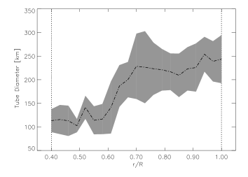
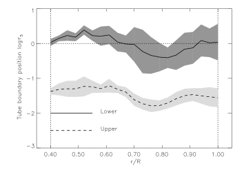
Figure 1.: Left panel: flux tube diameter as a function of the sunspot normalized radial distance in the penumbra. Right panel: radial variation of the lower (solid line) and upper (dashed) flux tube’s boundaries in the optical depth scale. Both figures from Borrero et al. 2006.

2. Problems in thick embedded flux tubes

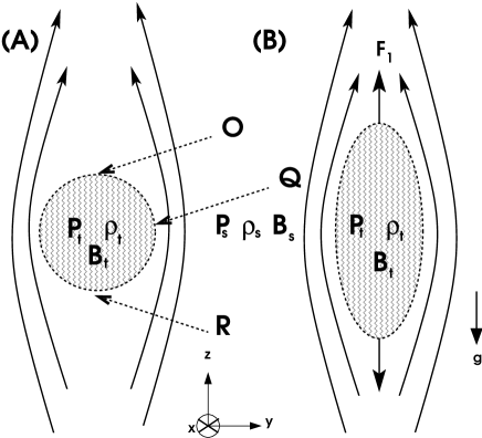
Figure 2.: Panel A (left): a homogeneous flux tube with density $\rho_{t}$ and pressure $P_{t}$ and horizontal (with respect to the vertical in the solar surface) magnetic field ${\rm{\bf{B_{t}}}}=(B_{tx},0,0)$, is place in a homogeneous environment with $\rho_{s}$ and $P_{s}$ where the magnetic field is vertical: ${\rm{\bf{B_{s}}}}=(0,B_{sy},B_{sz})$. The external field lines bend around the flux tube, creating tension forces that stretch the flux tube vertically (right panel B).

When a horizontal (initially homogeneous) magnetic flux tube ${\rm{\bf{B_{t}}}}$ is embedded in an external vertical magnetic field ${\rm{\bf{B_{s}}}}$, this external or surrounding field has to bend aside in order to accommodate the flux tube. A situation like this is depicted in Fig. 2 (panel A). The component of the magnetic field vector along the direction perpendicular to the flux tube’s surface vanishes for both the flux tube and surrounding field. This leads to total pressure balance between them:

$$P_{t}^{*}+\frac{B_{t}^{2*}}{8\pi}=P_{s}^{*}+\frac{B_{s}^{2*}}{8\pi}$$ (1)

where the symbol ^∗ indicates the boundary or interface between the flux tube and the magnetic surrounding atmosphere. On the laterals of the flux tubes (point Q in Fig. 2) we have:

$$P_{t}-P_{s}=\frac{B_{sz}^{2}-B_{tx}^{2}}{8\pi}$$ (2)

while on top and at the bottom of the flux tube (points O and points R in Fig. 2) since the external magnetic field vanishes completely we have:

$$P_{t}-P_{s}=-\frac{B_{tx}^{2}}{8\pi}$$ (3)

Any $P_{t}-P_{s}$ that balances Eq. 2 unbalances Eq. 3 in the amount of $B_{sz}^{2}/8\pi$. This imbalance induces net forces at the top and the bottom the flux tube that tend to stretch it vertically:

$${\rm{\bf{F}}}_{1}^{O} = \frac{B_{sz}^{2}}{8\pi R}{\rm{\bf e_{\rm z}}}$$ (4)

$${\rm{\bf{F}}}_{1}^{R} = -\frac{B_{sz}^{2}}{8\pi R}{\rm{\bf e_{\rm z}}}$$ (5)

These forces causes the flux tube to expand vertically in a time scale of

$$t_{\rm expan}=\frac{l}{v}\sim\frac{R}{v_{a}}\sim\frac{R}{B}\sqrt{4\pi\rho}\sim 20\;\;{\rm s}$$ (6)

where we assumed a flux tube radius of $R=100$ km, a typical density of $\rho=3\times 10^{-7}$ g cm^-3 and a field strength of $B=1000$ Gauss.

If nothing stops this process, the flux tube upper boundary will indefinitely move upwards and the bottom one will move downwards (see panel B in Fig. 2). This will end up breaking our idea of flux tube and of uncombed penumbra, since the gradients at flux tube’s boundaries (needed in the uncombed model to create NCP) will disappear from the regions in which the spectral lines are formed. In the following we will consider if this stretching process might be kept within limits.

3. Flux tubes in convectively stable layers

Let us assume that, as a consequence of the vertical stretching anticipated in the previous section, the upper part of our initially homogeneous flux tube rises from a height $z_{0}$ to a height $z$. If the atmosphere is subadiabatic (superadibatic index $\delta<0$), a restoring force will try to bring back the flux tube to its original position $z_{0}$:

$${\rm{\bf{F}}}_{2}^{O} = \frac{\rho g\delta\Delta z_{o}}{H_{p}}{\rm{\bf e_{\rm z}}}$$ (7)

where $H_{p}=P/\rho g$ is the pressure scale height. Note that ${\rm{\bf{F}}}_{2}^{O}$ opposes to ${\rm{\bf{F}}}_{1}^{O}$ (Eq. 4) since $\Delta z>0$ and $\delta<0$. The main question that rises now is: how much do the upper portions of the flux tube rise before the anti-buoyant restoring force compensates the magnetic forces ? This can be estimated by comparing Eq. 4 and Eq. 7:

$$\frac{\Delta z}{H_{p}}=-\frac{B_{sz}^{2}}{8\pi R\rho g}\frac{1}{\delta}\sim-\frac{0.75}{\delta}$$ (8)

Using a $\delta=-0.4$ (ideal gas at a constant temperature; see Moreno-Insertis & Spruit 1989) and $B_{sz}=1250$ Gauss we deduce that the vertical stretching occurring to the upper region of the flux tube is of the order of one or two pressure scale heights $\Delta z\sim H_{p}=P/\rho g\sim 100-200$ km. At this height its density will be $1-\delta$ times the density of the surrounding magnetic atmosphere.

This value for the vertical stretching is at the limits of what is needed to keep the flux tube boundary within the spectral line forming region. Futhermore, these estimates have been done for the case of the top and bottom of the flux tube. As we move towards the sides (point Q is Fig. 2) the vertical stretching is would be smaller.

Similarly we can argue that the stretching of the lower portions of the flux tube will not grow exponentially if these are less dense that the surrounding atmosphere (since $\Delta z<0$). When both conditions (upper and lower boundaries of the flux tube) are brought together, we end up with a non homogeneous flux tube. However, the lower boundary of the flux tube appears to be located near the continuum forming layers (Fig. 1; right panel), where the assumption of $\delta<0$ is not completely justified.

Note that $B_{sz}$ in Eq. 8 decreases strongly towards the outer penumbra, where the external field becomes weak and inclined $B_{sz}\sim 650$ and therefore $\Delta z/H_{p}\sim-0.2/\delta$. Near the umbra however, $B_{sz}$ reaches values as high as $1700$ Gauss and the vertical stretching is so large that the flux tube is likely to break disappear. High spatial resolution images of the sunspot penumbra reveal that often, when the penumbral filaments pour into the umbra, they break into two individual filaments that continue moving inwards and form umbral dots. The details presented here offer a scenario that might account for this process.

4. Conclusions

We have shown, using simple estimates that in a convectively stable atmosphere the vertical stretching of horizontal flux tubes, embedded in a penumbral field, is limited by buoyancy. It would be of considerable interest to use numerical simulations to confirm that the vertical stretching is compatible with the uncombed penumbral model.

Acknowledgments.

Thanks to Rolf Schlichenmaier and Tom Bogdan for useful discussions.

References

- (1) Borrero, J.M., Lagg, A., Solanki, S.K., Frutiger, C., Collados, M. & Bellot Rubio, L.R., 2003 in High Resolution Solar Observations: preparing for ATST, eds. A. Pestov & H. Uitenbroek, (ASP Conf. Ser. 286), 235
- (2) Borrero, J.M., Solanki, S.K., Bellot Rubio, L.R., Lagg, A. & Mathew, S.K. 2004, A&A, 422, 1093
- (3) Borrero, J.M., Solanki, S.K., Lagg, A., Collados, M. 2005, A&A, 436, 333
- (4) Borrero, J.M., Solanki, S.K., Lagg, A., Socas-Navarro, H. & Lites, B. 2006, A&A (in press)
- (5) Kippenhahn, R. & Möllenhoff, C., 1975, Elementare Plasmaphysik (Zürich, Wissenschaftsverlag)
- (6) Langhans, K., Scharmer, G., Kiselman, D., Löfdahl, M. & Berger, T. 2005, A&A, 436, 1087
- (7) Martínez Pillet, V. 2000, A&A, 361, 734
- (8) Mathew, S., Lagg, A., Solanki, S.K., et al. 2003, A&A, 403, 695
- (9) Moreno-Insertis, F. & Spruit, H.C. 1989, ApJ, 342, 1158
- (10) Müller, D.A.N., Schlichenmaier, R., Steiner, O. & Stix, M. 2002, A&A, 393, 305
- (11) Montesinos, B. & Thomas, J. 1997, Nature, 390, 485
- (12) Rouppe van der Voort, L., Löfdahl, M.G., Kiselman, D. & Scharmer, G.B. 2004, A&A, 414, 717
- (13) Scharmer, G., Gudiksen , B.V., Kiselman, D., et al. 2002, Nature, 420, 151
- (14) Schlichenmaier, R. & Collados, M. 2002, A&A, 381, 668
- (15) Schlichenmaier, R., Müller, D.A.N., Steiner, O. & Stix, M. 2002, A&A, 381, L77
- (16) Schlichenmaier, R. 2002, AN, 323, 303
- (17) Schlichenmaier, R., Jahn, K. & Schmidt, H.U. 1998a, A&A, 337, 897
- (18) Schlichenmaier, R., Jahn, K. & Schmidt, H.U. 1998b, ApJ, 483, L121
- (19) Schlichenmaier, R., Bruls, J., & Schüssler, M. 1999, A&A, 349, 961
- (20) Schlichenmaier, R. & Solanki, S.K. 2003, A&A, 411, 257
- (21) Spruit, H.C & Scharmer, G. 2006, A&A (in press)
- (22) Solanki, S.K. 2003, A&ARv, 11, 153
- (23) Solanki, S.K., & Montavon, C.A.P. 1993, A&A, 275, 283
- (24) Sütterlin, P., Bellot Rubio, L.R. & Schlichenmaier, R. 2004, A&A, 424, 1049
- (25) Thomas, J. & Montesinos, B. 1993, ApJ, 407, 398
- (26) Westendorp Plaza, C., del Toro Iniesta, J.C., Ruiz Cobo, B. & Martínez Pillet, V. 2001a, ApJ, 547, 1148
- (27) Westendorp Plaza, C., del Toro Iniesta, J.C., Ruiz Cobo, B. et al. 2001b, ApJ, 547, 1130