X–ray spectral properties of AGN in the Chandra Deep Field South

We present a detailed X–ray spectral analysis of the sources in the 1Ms catalog of the Chandra Deep Field South (CDFS) taking advantage of optical spectroscopy and photometric redshifts for 321 extragalactic sources out of the total sample of 347 sources. As a default spectral model, we adopt a power law with slope $\Gamma$ with an intrinsic redshifted absorption $N_{H}$, a fixed Galactic absorption and an unresolved Fe emission line. For 82 X–ray bright sources, we are able to perform the X–ray spectral analysis leaving both $\Gamma$ and $N_{H}$ free. The weighted mean value for the slope of the power law is $\langle\Gamma\rangle\simeq 1.75\pm 0.02$, and the distribution of best fit values shows an intrinsic dispersion of $\sigma_{int}\simeq 0.30$. We do not find hints of a correlation between the spectral index $\Gamma$ and the intrinsic absorption column density $N_{H}$.

We then investigate the absorption distribution for the whole sample, deriving the $N_{H}$ values in faint sources by fixing $\Gamma=1.8$. We also allow for the presence of a scattered component at soft energies with the same slope of the main power law, and for a pure reflection spectrum typical of Compton–thick AGN. We detect the presence of a scattered soft component in 8 sources; we also identify 14 sources showing a reflection–dominated spectrum. The latter are referred to as Compton–thick AGN candidates.

By correcting for both incompleteness and sampling–volume effects, we recover the intrinsic $N_{H}$ distribution representative of the whole AGN population, $f(N_{H})dN_{H}$, from the observed one. $f(N_{H})$ shows a lognormal shape, peaking around $log(N_{H})\simeq 23.1$ and with $\sigma\simeq 1.1$. Interestingly, such a distribution shows continuity between the population of Compton–thin and that of Compton–thick AGN.

We find that the fraction of absorbed sources (with $N_{H}>10^{22}$ cm^-2) in the sample is constant (at the level of about $75$%) or moderately increasing with redshift. Finally, we compare the optical classification to the X–ray spectral properties, confirming that the correspondence of unabsorbed (absorbed) X–ray sources to optical Type I (Type II) AGN is accurate for at least 80% of the sources with spectral identification (1/3 of the total X-ray sample).

1 Introduction

Deep X–ray surveys with Chandra (Brandt et al. 2001; Rosati et al. 2002; Cowie et al. 2002; Alexander et al. 2003; Barger et al. 2003) and XMM (Hasinger et al. 2001) showed that the so called X–ray background (XRB) is mainly provided by Active Galactic Nuclei (AGN) both in the soft (0.5–2 keV) and in the hard (2–10 keV) band. In particular, major progress has been made in the hard band, for which the sources known before Chandra were providing only $\sim 30$% of the XRB (Cagnoni et al. 1998; Ueda et al. 1999a). While some evidence of spectral hardening was found towards faint fluxes (e.g. Della Ceca et al. 1999), most of the X-ray sources were identified with Broad Line AGN with a typical X-ray spectral slope of $\Gamma=1.7-2.0$, steeper than that of the XRB ($\Gamma\simeq 1.4$). On the contrary, the source population discovered by Chandra and XMM at fluxes below $\sim 10^{-13}-10^{-14}$ erg cm^-2 s^-1 in the hard band, is constituted mostly by obscured AGN with a hard spectrum, and provides the solution to the “spectral paradox” as predicted by the XRB synthesis models (Setti & Woltjer 1989, Madau, Ghisellini & Fabian 1993; Comastri, Setti, Zamorani & Hasinger 1995; Gilli, Salvati & Hasinger 2001). The detection limit reached in the hard band in the 2Ms exposure of the Chandra Deep Field North is $S\simeq 2\times 10^{-16}$ erg s^-1 cm^-2 (Alexander et al. 2003) and a factor 2 higher in the 1Ms exposure of the Chandra Deep Field South (CDFS, Rosati et al. 2002; Giacconi et al. 2002). The XRB is now resolved at the level of $\sim 80$% in the 1–2 and 2–8 keV bands (see Hickox & Markevitch 2005), with the AGN providing the large majority of the resolved fraction. While a non–negligible part of the unresolved fraction in the soft band is expected to be contributed by a diffuse warm intergalactic medium (e.g., Cen & Ostriker 1999), Worsley et al. (2004; 2005) pointed out that at $E>6$ keV less and less of the hard XRB is resolved, showing that a significant population of strongly absorbed, possibly Compton–thick sources, preferentially at $z<1$, is still not observed (see also Comastri 2004; Brandt & Hasinger 2005).

The two Chandra Deep Field Surveys lead to the detection of several populations of X–ray extragalactic sources: unabsorbed AGN (defined as sources with absorbing column densities $N_{H}<10^{22}$ cm^-2), usually identified with optical Broad Line (Type I) AGN and QSO; absorbed AGN (with column densities $N_{H}\geq 10^{22}$ cm^-2), optically identified mostly as narrow line (Type II) AGN, distributed around moderate redshifts $z\sim 1$ (see Barger et al. 2002; Szokoly et al. 2004); X–ray bright, optically normal galaxies (XBONG, see Comastri et al. 2001) which generally harbor obscured AGNs; high redshift Type II QSO (see Norman et al. 2002; Stern et al. 2002; Mainieri et al. 2005a; Ptak et al. 2005); starburst and quiescent galaxies at $z<1$ (Bauer et al. 2002; Hornschemeier et al. 2003; Norman et al. 2004), which contribute to the XRB only $2-3$% in energy, but they are expected to outnumber the AGN at fluxes below $1\times 10^{-17}$ erg cm^-2 s^-1 (Bauer et al. 2004a). In this Paper we will focus on the X–ray properties of the AGN population, in order to provide a baseline for possible models of the AGN formation and evolution.

Tentatively, the different classes of AGN–powered X–ray sources can be associated to three phases: a first phase of strong accretion onto the massive black hole, characterized by high intrinsic absorption and intense star formation (for recent evidence in the submm range see Alexander et al. 2005a), followed by an unobscured phase, and subsequent fading (see Fabian 1999; Granato et al. 2004). A test of this or other possible scenarios for the accretion history and galaxy formation in the Universe, requires a good knowledge of the distribution of the X–ray properties of the AGN population, in particular intrinsic luminosity and intrinsic absorption as a function of cosmic epoch, as well as their relation with the optical properties. The distribution of the intrinsic absorption, $N_{H}$, is known only for local, optically selected Seyfert II galaxies (Risaliti et al. 1999). These local samples, selected to be complete as a function of intrinsic luminosity, typically include medium or low luminosity sources, and about 50% of them are Compton–thick. Difficulty of assembling large unbiased AGN sample as a function of intrinsic luminosity, has hampered attempts to measure the $N_{H}$ distribution. The $N_{H}$ distribution and the evolution of the fraction of absorbed sources, has been investigated recently by Ueda et al. (2003) from a combination of surveys from HEAO1, ASCA and Chandra. Their sample is dominated by bright, low absorption AGN, and their $N_{H}$ distribution is broadly peaked above $N_{H}>10^{22}$ cm^-2. Except for a few objects with good photon statistics, Ueda et al. use the redshift and the hardness ratio to derive the intrinsic luminosity distribution in the 2–10 keV band as a function of redshift, without performing a single–source analysis. Similar results have been recently obtained by La Franca et al. (2005) on the basis of the HELLAS2XMM sample combined with other catalogs. At brighter fluxes, other investigations are under way both with Chandra and XMM in wide, shallower surveys (ChaMP, Green et al. 2004; Silverman et al. 2005; XMM–BSS, Della Ceca et al. 2004; CLASXS, Yang et al. 2004, Steffen et al. 2004; HELLAS2XMM, Baldi et al. 2002; Perola et al. 2004). We believe that these X–ray surveys, designed to bridge the gap between the pencil beam, deepest surveys and the wide shallow ones from previous missions, are probably biased against heavily absorbed faint AGN, whose fraction is expected to increase towards fainter fluxes. On the other hand, optical surveys can actually discover heavily obscured AGNs at moderate redshift ($z<1.3$) but only through extensive optical spectroscopy of large sample of galaxies, such as the SDSS, among which type II AGNs can be identified from the strong narrow emission lines (for example, [OII]$\lambda$3727$\AA$ or [OIII]$\lambda$5007$\AA$). In the absence of high–sensitivity X–ray surveys above 10 keV, we propose that the search for the still missing strongly absorbed AGN population can be best performed through a detailed spectral analysis of faint sources detected in very deep X–ray surveys.

In this Paper, we present a systematic study of the X–ray spectra of all the sources in the CDFS, taking advantage of spectroscopic (Szokoly et al. 2004) and photometric (Zheng et al. 2004; Mainieri et al. 2005a) redshifts from the optical follow–up program with the ESO–VLT. Given the flux limits in the CDFS ($5.5\times 10^{-17}$ and $4.5\times 10^{-16}$ erg cm^-2 s^-1 in the soft and hard band respectively), the 347 sources detected (346 from the catalog of Giacconi et al. 2002 plus one added in Szokoly et al. 2004) are mostly AGN, with a fewer number of normal or star forming galaxies with respect to CDFN, where, thanks to the lower flux limits, normal galaxies start to be a significant fraction of the faint source population. The Paper is structured as follows. In §2 we briefly describe the X–ray and the Optical data. In §3 we describe our X–ray spectral analysis procedure, after dividing the sample into two subsamples based on the counts statistics. In §4 we present the X–ray spectral analysis of the X–ray bright sample, focusing on the slope of the power law component. In §5 we present the X–ray spectral analysis for the whole sample of 321 sources with measured redshift and total luminosity $L_{X}>10^{41}$ erg s^-1 (we exclude the faintest luminosity bin which is doninated by normal galaxies), focusing on the intrinsic absorption. In §6 we discuss the distributions of the X–ray spectral properties after correcting for incompleteness and sampling–volume effects, deriving in particular the intrinsic absorption distribution. This allows us to estimate the fraction of absorbed sources in our sample as a function of epoch. Finally, in §7 we compare the X–ray and optical properties, revisiting the comparison of the Optical vs X–ray classification scheme proposed by Szokoly et al. (2004). Our conclusions are summarized in §8. Luminosities are quoted for a flat cosmology with $\Lambda=0.7$ and $H_{0}=70$ km/s/Mpc (see Spergel et al. 2003).

2 The data

The 1Ms dataset of the CDFS is the result of the coaddition of 11 individual Chandra ACIS–I (Garmire et al. 1992; Bautz et al. 1998) exposures with aimpoints only a few arcsec from each other. The nominal aim point of the CDFS is $\alpha=$3:32:28.0, $\delta=-$27:48:30 (J2000). The reduction and analysis of the X–ray data are described in Giacconi et al. (2001), Tozzi et al. (2001) and Rosati et al. (2002). The final image covers 0.108 deg², where 347 X–ray sources are identified (the catalog is presented in Giacconi et al. 2002). Here we use an updated X-ray data reduction, where we used Ciao 3.0.1 and CALDB2.26, therefore including the correction for the degraded effective area of ACIS–I chips due to material accumulated on the ACIS optical blocking filter at the epoch of the observation. We also apply the recently released, time–dependent gain correction.

We briefly recall the main steps of the spectral analysis of the reduced data. First we extract the photon files and the spectrum (pha file) for every source in our catalog, along with the corresponding background. The area of extraction of each source, as described in Giacconi et al. (2001), is defined as a circle of radius $R_{s}=2.4\times FWHM$ (with a minimum radius of 5 arcsec). The FWHM is modeled as a function of the off–axis angle to reproduce the broadening of the PSF. The background is extracted from an annulus with outer radius $R_{S}+12^{\prime\prime}$ and an inner radius of $R_{S}+2^{\prime\prime}$, after masking out other sources. Each background spectrum samples more than 400 photons in the 0.5–7 keV range. We create a response matrix and an ancillary response matrix for each source. To do that, we first create the two matrices in the source position in each of the 11 observations of the CDFS (therefore the effect of the degraded effective area of ACIS–I chips is applied individually to each pointing). Finally we sum the 11 files weighting them for the exposure time of each exposure. We notice that most of the sources show variability (see Paolillo et al. 2004), therefore our measured fluxes and luminosities are time–averaged on the observation epochs. We also stress that, assuming there is no significant changes in the spectra, we correctly measure the spectral shape of each source, since the response matrices are time–averaged on the same epochs, keeping track in the most detailed way of the characteristics of the different regions and the different conditions of the detector at the time of the observations.

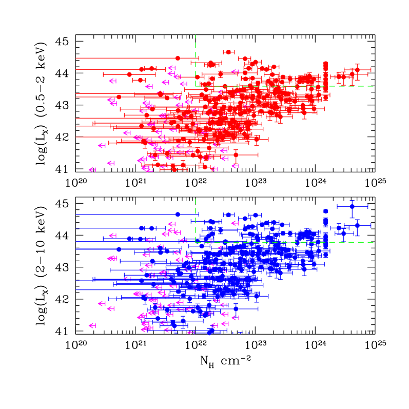
Figure 13: Unabsorbed rest–frame luminosities in the soft (upper panel) and in the hard (lower panel) band plotted versus the intrinsic absorption. Upper limits (1 $\sigma$) are used for for measures consistent with $N_{H}=0$ within 1 $\sigma$. Error bars correspond to 1 $\sigma$. Upper right corners outlined by the dashed lines show the locus of QSO–II, defined as sources with $L_{X}>10^{44}$ erg s^-1 and $N_{H}>10^{22}$ cm^-2 (as opposed to the criterion $HR>-0.2$ and $L_{X}>10^{44}$ erg s^-1 used in Szokoly et al. 2004).

The spectroscopic identification program carried out with the ESO-VLT is presented in Szokoly et al. (2004). The optical classification is based on the detection of high ionization emission lines. The presence of broad emission lines (FWHM larger than 2000 km/s) like Mg_II, C_III, and, at large redshifts, C_IV and Ly$\alpha$, identifies the source as a Broad Line AGN (BLAGN), Type–1 AGN or QSO in the simple unification model (Antonucci 1993). The presence of unresolved high ionization emission lines (like O_III, Ne_V, Ne_III or He_II) identifies the source as a High Excitation line galaxy (HEX), often implying an optical Type–2 classification. Objects with unresolved emission lines consistent with an H_II region spectrum are classified as Low Excitation Line galaxies (LEX), implying sources without signs of nuclear activity in the optical (however, discriminating between a Seyfert II galaxy and an $HII$ region galaxy involves the measure of line ratio as shown in Veilleux & Osterbrock (1987), which is not used here as a classification scheme, considering also that their classification scheme relies on lines which are not visible in optical spectra from the ground at $z>0.7$). Objects with typical galaxy spectrum showing only absorption lines are classified as ABS; among the last two classes we expect to find star–forming galaxies or Narrow Line Emission Galaxies, but also hidden AGN. The optical identification is flagged according to the quality of the optical information. Quality flags $Q\geq 1$ indicates spectroscopic redshifts (see Table X–ray spectral properties of AGN in the Chandra Deep Field South). In several cases, the optical spectral properties do not allow us to obtain a secure determination of the spectral type. As shown in Szokoly et al. (2004), the optical classification scheme is failing in identifying an AGN in about 40% of the X-ray sources optically classified as LEX or ABS. Therefore, an X–ray classification scheme, based on the source hardness ratio and observed X–ray luminosity, was worked out by Szokoly et al. (2004) and compared with the optical one (see their Fig. 13). In Section §7 we will reconsider this X–ray classification scheme using the intrinsic luminosities (as opposed to observed ones) and intrinsic absorption (as opposed to the hardness ratio).

Optical and near-IR images of the CDFS are also used to derive photometric redshifts for all the remaining X–ray sources. Using the widest multiwavelength photometry available today, Zheng et al. (2004) and Mainieri et al. (2005a) derived photo–z for the whole sample of sources but four. Photometric redshifts are obtained from different methods labelled with different quality flags (see Zheng et al. 2004 for details). When we have consistent redshift from more than one method, the corresponding quality flag is the sum of the single $Q$ (always less than 1 for photometric redshift). Given the good agreement of photometric redshifts with spectroscopic ones (see Zheng et al. 2004), we do not divide our sample according to the optical spectra quality. Indeed, our statistical analysis is not expected to be significantly affected by uncertainties in the photometric redshifts. Uncertainties in the redshift estimate may instead significantly affect the search for the Fe line, as we discuss later.

The total number of sources with spectral or photometric redshift $z>0$ is 336 over a total of 347 X–ray detections. Besides the 4 X-ray sources without any redshift estimate, we indeed identify 7 stars with good optical spectra. Therefore the spectral completeness of our sample of extragalactic sources is $\sim 99$ %. Since we want to focus on AGN, we adopt a conservative criterion and exclude 15 sources with total luminosity in the 0.5–10 keV band $L_{X}<10^{41}$ erg s^-1, a luminosity range which is expected to be dominated by normal or star forming galaxies. We note that the higher luminosiy range $10^{41}<L_{X}<10^{42}$ erg s^-1 may include several star forming galaxies as well, with star formation rate of the order of $100M_{\odot}$/yr. However, we keep all the sources in the luminosiy range $10^{41}<L_{X}<10^{42}$ erg s^-1 to include any possible low–luminosity AGN in the sample. The final sample amounts to 321 sources. The redshifts with the corresponding spectral quality are shown along with the results from the X–ray spectral fits in Table X–ray spectral properties of AGN in the Chandra Deep Field South.

3 The X–ray spectral analysis

3.1 Fitting strategy

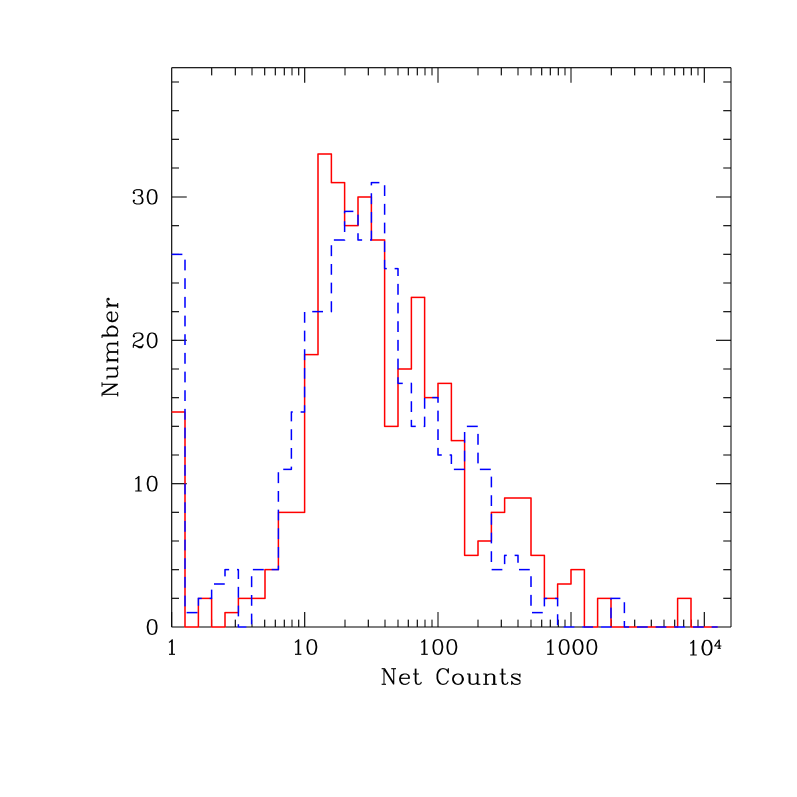
Figure 1: Distribution of the net detected counts for all the sources in the sample (solid line: 0.5–2 keV band counts; dashed line: 2–7 keV band counts).

We use XSPEC v11.3.1 (see Arnaud 1996) to perform the spectral fits. The ability of obtaining a reliable fit depends on the X–ray spectral quality, or, in simpler terms, on the signal to noise of the spectrum under analysis. The distribution of the net counts in the 0.5–7 keV band for all the sources in our sample, peaks below $\simeq 100$ (see Figure 1). The mean value of the net detected counts in the total 0.5–7 keV band for all the sources in our sample (including the two X–ray brightest sources in the sample, with about 10000 counts each) is $\simeq 240$ counts, while the median is much lower $\simeq 70$ counts.

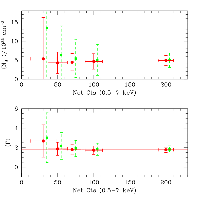
Figure 2: The average best–fit parameters (with rms dispersion) for a source with intrinsic $N_{H}=5\times 10^{22}$ cm^-2 and $\Gamma=1.7$ at $z=1$ fitted with Cash statistics (filled circles, continuous error bars) and $\chi^{2}$ (filled squares, dashed error bars) versus the number of net detected counts in the 0.5-7 keV band. The $\chi^{2}$ points are slightly shifted along the x–axis for clarity. The same source is simulated 1000 times for five different intrinsic normalizations, resulting in a different average number of net detected counts.

Therefore, the strategy for the X–ray spectral analysis must be appropriate for the low counts regime. In performing the spectral fits we used an extension of the Cash statistics which makes use of both the source and background spectral files. Cash statistics is applied to unbinned data, and therefore exploit the full spectral resolution of the ACIS–I instrument, allowing better performance with respect to the canonical $\chi^{2}$ analysis, particularly for low signal–to–noise spectra (Nousek & Shue 1989). In order to assess the ability of our fitting procedure in a typical case (a source with $\Gamma=1.7$ and $N_{H}=5\times 10^{22}$ cm^-2 at $z=1$) we run several simulations for different input fluxes, in which we try to recover the input parameters with two different fitting procedures: Cash statistics (unbinned) and the classic $\chi^{2}$ statistics with a binning of 10 photons per bin. The results are summarized in Figure 2. Note that we are forced to use a binning of 10 photons (as opposed to the commonly used binning of 20 photons) in order have a reasonable number of bins to perform the $\chi^{2}$ fits in the low–counts regime. Such a small binning is known to give inappropriate weights for the $\chi^{2}$ analysis, therefore we do not mean to present a detailed comparison of the two methods. Indeed, here we just explore the effects that their use would have in the spectral analysis of our sample. For the $\chi^{2}$ statistics, we find that for sources with a number of net counts equal or larger than 50, the input parameters are recovered with very good accuracy, while for lower values, the peak of the distribution of the best–fit–values starts to depart from the input value. The shift in the distribution of the best–fit values is a consequence of the binning, which, especially in the case of low–counts statistics, acts as an effective smoothing on the spectrum. On the other hand, the distribution of the best–fit values with Cash–statistics appears to be closer to the input values. In addition, the rms dispersion of best–fit values is significantly lower with respect to the $\chi^{2}$ statistics. We also checked that the confidence levels for the Cash–statistics can be defined as in the $\chi^{2}$–statistics (i.e., $\Delta C=1.0$ corresponds to 1 $\sigma$, $\Delta C=2.7$ corresponds to 90% c.l. for one interesting parameter). Therefore we choose to quote only the best fit values obtained with the Cash statistics.

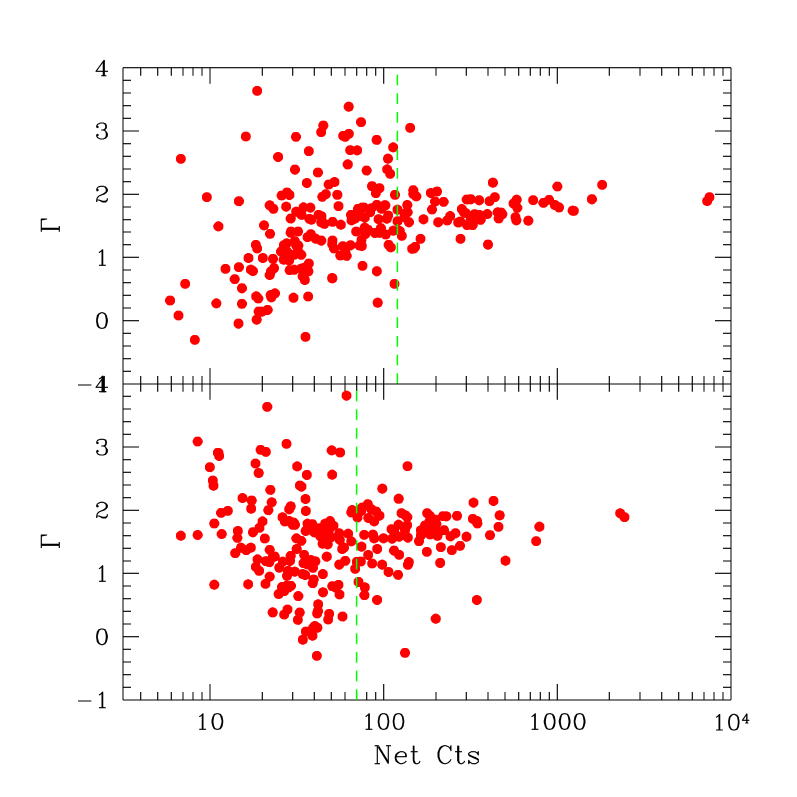
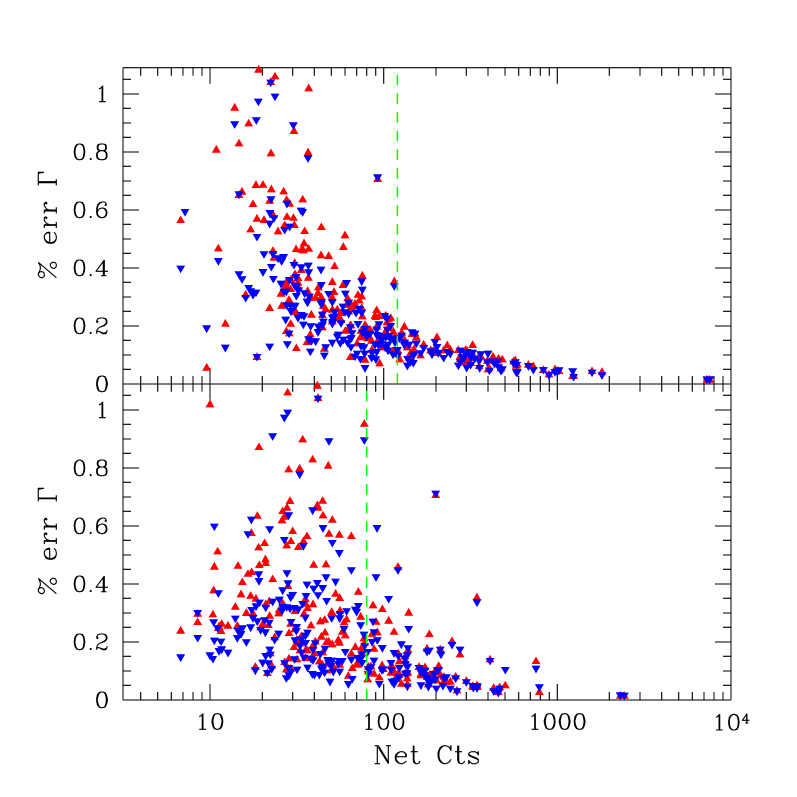
Figure 3: Left: best fit values of the spectral slope $\Gamma$ as a function of the net counts in the soft (top panel) and hard (bottom panel) bands (for sources with more than 40 net counts in the 0.5–7 keV band). Right: fractional statistical error ($1\sigma$ c.l.) on $\Gamma$ as a function of net counts in the soft (top panel) and hard (bottom panel) band (upper and lower errors are shown as triangles and upside–down triangles respectively). Vertical dashed lines are the thresholds adopted to select the bright X–ray sample (82 sources with more than 120 net counts in the soft band or more than 80 in the hard band, or more than 170 counts overall).

Of course, the weak signal of our faintest sources limits the ability to perform a fit keeping all the spectral parameters free. To determine the validity of our approach, we first run the fit for our default model with three free parameters ($N_{H}$, $\Gamma$ and normalization) on all the sources with more than 40 net detected counts in the total 0.5–7 keV band. First we focus on the distribution of the best–fit values for $\Gamma$ as a function of the net counts (see Figure 3, left). We notice that for sources detected with a large number of counts (larger than $\simeq 200$) the spectral slope is almost constant. On the other hand, at low counts, the best fit spectral slope $\Gamma$ shows an apparent trend associated with a significant increase in the dispersion on $\Gamma$ (see Figure 3, right): lower values at lower soft counts, higher values at lower hard counts. In principle this is expected, since most of the sources with few soft counts are among the hardest sources, and they can be fitted with a flat power law, and viceversa the softest sources can be fitted with a very steep power law. However, we argue that this behaviour may be affected by the poor statistics. To avoid any possible bias induced by the low statistics, we conservatively define an X-ray bright sample by considering those sources exceeding at least one of these thesholds: 170 total counts, 120 soft counts, 80 hard counts. As we can see in Figure 3b, the threshold on the soft counts is particularly efficient in selecting sources for which the statistical error on $\Gamma$ is smaller than 20% (about 10% in average). The bright sample, constituted by 82 sources, will be used to investigate both the intrinsic spectral slope $\Gamma$ and the intrinsic absorption $N_{H}$. We remark here that the bright sources are selected on the basis of the net detected counts, and not on the basis of the energy flux; among the brigth sample, we find sources with fluxes larger than $4\times 10^{-16}$ erg s^-1 cm^-2 in the soft and $1.3\times 10^{-15}$ erg s^-1 cm^-2 in the hard band. As for the remaining 3/4 of the sample, we decide to fix the slope to the canonical value of $\Gamma\simeq 1.8$ (see Turner et al. 1997), which is, in turn, very close to the average value measured for our bright sample (as shown in §4), and focus on the intrinsic absorption.

3.2 Spectral models

We assume a default spectral model based on a power law (XSPEC model pow) and intrinsic absorption at the source redshift (XSPEC model zwabs) with redshift frozen to the spectroscopic or photometric value. Also, we search for the Fe K$\alpha$ line at 6.4 keV rest–frame, which is one of the most common features of AGN X–ray spectra. To investigate the presence of such a line, we added a redshifted unresolved Gaussian line at $6.4/(1+z)$ keV (Nandra & Pounds 1994). We also take into account the local Galactic absorption (XSPEC model tbabs) with a column density frozen to $N_{H}=8\times 10^{19}$ cm^-2 (from Dickey & Lockman 1990). The fits are performed on the energy range 0.6–7 keV. We cut below 0.6 keV to avoid uncertainties in the ACIS calibration in an energy range which anyway offers a small effective area. At high energies, the efficiency of Chandra is rapidly decreasing, and the energy bins at more than 7 keV are dominated by the noise for the large majority of the sources in our flux range. It has recently been shown that a methylen layer on the Chandra mirrors increases the effective area at energies larger than 2 keV (see Marshall et al. 2003). This has a small effect on the total measured fluxes, but it can have a non-negligible effect on the spectral parameters. To correct for this, we include in the fitting model a “positive absorption edge” (XSPEC model edge) at an energy of 2.07 keV and with $\tau=-0.17$ (Vikhlinin et al. 2005). This multiplicative component artificially increases the hard fluxes by $\simeq 3.5$%, therefore the final hard fluxes and luminosities computed from the fit are corrected downwards by the same amount.

In some cases, the fit with a simple absorbed power law may not be a good description of the X–ray spectrum. On the other hand, our limited counts statistics does not allow us to investigate for complex spectral shapes as often observed in AGN. However, we identify two possible additional spectral models. A first spectral model we investigate is the presence of a soft component in addition to the absorbed power law, as often found in the X-ray spectra of Seyfert 2 galaxies (e.g. Turner et al. 1997). Such a soft component can arise from several physical processes, like nuclear radiation scattered by a warm medium (the so-called ”warm mirror”, e.g. Matt et al. 1996), or nuclear radiation leaking through the absorber. In this cases, the soft component is expected to have the same spectral slope of the main power law. Here we do not consider the soft excess possibly due to thermal emission or comptonization of soft photons, as found in bright quasars (see Porquet et al. 2004). Thus, we repeated the fits simply adding to the Compton–thin model an unabsorbed power law component with slope equal to that of the main power law, requiring the intrinsic normalization of the soft component to be always less than 10% of the intrinsic normalization of the main power law. This last requirement embraces typical values both for a scattered component and for leaky absorbers (see Turner et al. 1997). This upper limit may exclude some leaky absorber with a low covering fraction, but at the same time helps us in avoiding false detections of high–normalization soft components implying spuriously high values of $N_{H}$ relative to the absorbed component. With this procedure, a soft component is detected with $\Delta C>2.7$ in 8 sources.

Moreover, when the intrinsic absorption is as high as $N_{H}\simeq 1.5\times 10^{24}$ cm^-2, the Compton optical depth is equal to unity and the directly transmitted nuclear emission is strongly suppressed in the Chandra soft and hard bands. In particular, for an intrinsic power–law spectrum with $\Gamma=1.8$, the fraction of transmitted photons is less than $2\%$ in the soft band up to redshift $z=2$. Absorption is less severe in the hard band, where for $z>1$ already a fraction of $10\%$ of the emitted photons are recovered. It is clear that only the intrinsically brightest, heavily absorbed high–redshift AGN can be detected by their transmitted nuclear emission. In this regime, a radiation component reflected by a cold medium, expected to be in average $6\%$ of the intrinsic power in the 2–10 keV band, starts to be important. For these Compton–thick sources, the most commonly observed spectrum is dominated by a Compton–reflection continuum from cold medium, usually assumed to be produced by the far inner side of the putative obscuring torus. This can be modeled with the XSPEC model pexrav (Magdziarz & Zdziarski 1995) plus the redshifted Fe K line.

The pexrav model often provides a better fit for the sources in our sample with a flat spectrum. For simplicity, we fix all the parameters to the default, typical values ($\Gamma=1.8$, reflection relative normalization=0, element and Fe abundance set to 1, cosine of inclination angle set to 0.45) but the normalization of the intrinsic power law spectrum. Our selection of Compton–thick candidates, then, is based on the comparison of the Cash–statistics obtained in the best fits with the zwabs pow model (with two free parameters, $N_{H}$ and normalization) with that obtained with the pure reflection model (with only one free parameter, the normalization). The difference $\Delta C$ is an indication of the goodness of the pexrav model with respect to the standard absorbed power law. Due to the different number of free parameters and the low signal-to-noise typical of our sources, we choose a threshold $\tilde{\Delta}C$ to select Compton–thick candidates after extensive simulations. The simulations procedure is described in Appendix B. We find that a threshold $\tilde{\Delta}C=2$ allows us to select a sample of Compton–thick candidates with a contamination fraction of about 20%. On the other hand, we also find that with our selection criteria, we may miss a fraction as high as 40% of the total Compton–thick population. Indeed, we find that, given the typical signal–to–noise of our sample, it is extremely difficult to efficiently select Compton–thick sources on the basis of the shape of the X–ray spectrum. We recognize that, in order to perform a careful search for Compton–thick candidates, other spectral features, like the Fe K line, or other wavelengths (like the submillimeter range of SCUBA) should be explored (see Alexander et al. 2005b). This goes beyond the goal of this Paper.

To summarize, we label as C–thin the sources for which the best fit model is a power law with intrinsic absorption; C–thick the sources for which the best fit is given by a pexrav model; finally Soft–C for sources whose best fit model includes a soft component with the same slope of the main power law. Finally, we always add a gaussian component to model the Fe K line, which, in case of no detection, gives a null or negligible contribution to the spectral shape.

4 Spectral slope for the bright sample

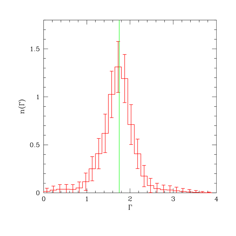
Figure 4: Distribution of the spectral slope $\Gamma$ for the X–ray bright sample (82/321 sources). Error bars are 1 $\sigma$ poissonian errors. The solid vertical line refers to the central value $\langle\Gamma\rangle=1.75$.

First, we consider only the X–ray bright sample of 82 sources with more than 120 net detected counts in the soft band or more than 80 in the hard band, and more than 170 net counts overall. Among them, only two sources with soft component are found, and no Compton thick candidates. We note that the low fraction of sources with significant soft component, lower than that in the local sample of Turner et al. (1997), may be ascribed to the high redshifts in our sample, for which the soft component is often shifted below 0.6 keV. We use this subsample (1/4 of the total sample) to investigate the behaviour of the spectral slope $\Gamma$. The normalized distribution of spectral slopes for the X–ray bright sample is shown in Figure 4. The distribution has been obtained by extracting the value of $\Gamma$ of each source $10^{4}$ times from the range allowed by the statistical error bars, assuming a gaussian error distribution. With this procedure, we weight each source in the histogram according to the statistical errors on $\Gamma$. Before computing the weighted mean value, we exclude the two brightest sources in the sample (about $10^{4}$ net counts each) which otherwise would dominate the statistics. We find that the weighted mean value for the spectral slope of the bright sample is $\langle\Gamma\rangle=1.75\pm 0.02$ (error bar refers to 1 $\sigma$ uncertainty on the mean value). While the typical error on a single measure is about $\Delta\Gamma\simeq 0.13$, the dispersion of the distribution of the best fit values is $\sigma\simeq 0.33$. Assuming that both statistical errors and the intrinsic dispersion in $\Gamma$ are distributed as a Gaussian, the intrinsic scatter is of the order of $\sigma_{int}\sim 0.30$. If we focus on the 30 brightest sources to decrease the statistical errors (still excluding the two sources with $\sim 10^{4}$ counts), the estimate of the intrinsic scatter decrease to $\sigma_{int}\sim 0.20$, and the weighted mean value is $\langle\Gamma\rangle=1.81\pm 0.01$.

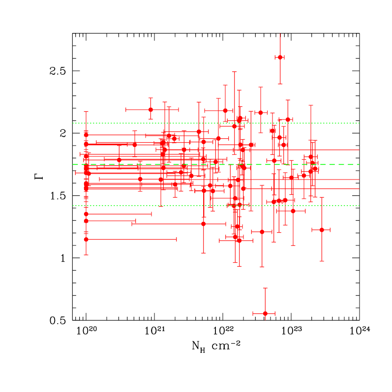
Figure 5: Scatter plot of the best fit values of $\Gamma$ and $N_{H}$ for the bright X–ray sample (82 sources). Error bars correspond to 1 $\sigma$. The dashed and dotted horizontal lines show the average value of $\Gamma$ and its rms dispersion respectively.

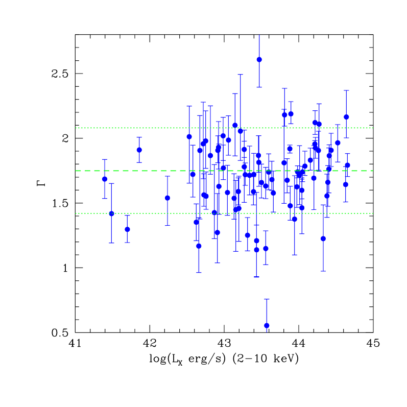
Figure 6: Scatter plot of the best fit values of $\Gamma$ versus unabsorbed hard rest–frame luminosities for the bright X–ray sample (82 sources). Error bars correspond to 1 $\sigma$. The dashed and dotted horizontal lines show the average value of $\Gamma$ and its rms dispersion respectively.

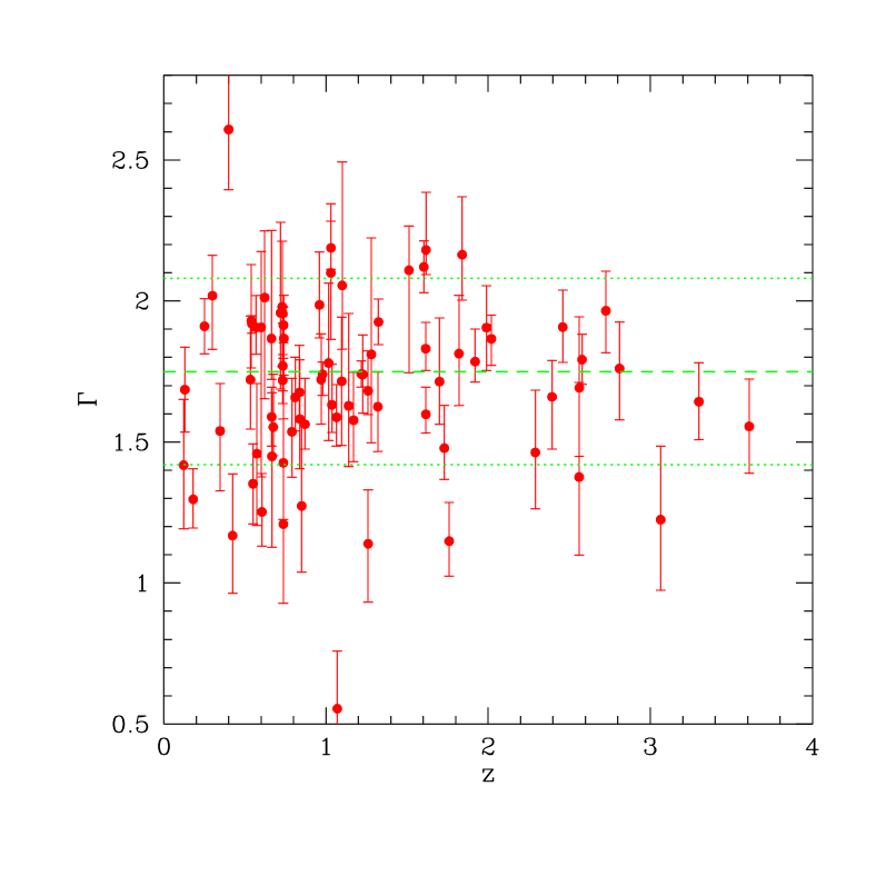
Figure 7: Scatter plot of the best fit values of $\Gamma$ versus redshift for the bright X–ray sample (82 sources). Error bars correspond to 1 $\sigma$. The dashed and dotted horizontal lines show the average value of $\Gamma$ and its rms dispersion respectively.

In Figure 5, we plot the best fit values of $\Gamma$ versus the best fit values of the intrinsic absorption $N_{H}$. We do not detect any correlation between $\Gamma$ and $N_{H}$ (Spearman Rank coefficient $SR\sim-0.04$). Note that if the intrinsic absorption is close to the Galactic value for the CDFS field ($N_{Hgal}\simeq 8\times 10^{19}$ cm^-2) we are not able to derive any meaningful value, due to the low–energy limit of our spectral range ($E>0.6$ keV). We considered these sources to be unabsorbed, plotting them at $N_{H}=10^{20}$ cm^-2 in our Figures. We detect no correlation between $\Gamma$ and the hard rest–frame intrinsic (unabsorbed) luminosity (see Figure 6). The Spearman Rank correlation is null also between $\Gamma$ and the redshift (see Figure 7).

From the analysis of the bright sample, we conclude that among our sources the intrinsic continuum is well approximated by a power law with $\Gamma\simeq 1.8$ (typical of Seyfert galaxies and AGN, as known also from ASCA studies of AGN, see Turner et al. 1997) at any epoch. On the other hand, it is well known that the flattening of the average spectrum of the sources at low fluxes in deep X–ray survey is due mainly to increasing intrinsic absorption (see Ueda et al. 1999b; Tozzi et al. 2001; Piconcelli et al. 2003; La Franca et al. 2005). In addition, previous studies found no hints for a change in the slope of the intrinsic power law as a function of epoch or luminosity (see also Mainieri et al. 2002; Piconcelli et al. 2003; Vignali et al. 2003). We conclude that the slope of the intrinsic power law can be assumed to be constant for all the AGN population, and, therefore, we choose to fix the spectral slope to $\Gamma=1.8$ when fitting the remaining fainter sources, focusing on the $N_{H}$ distribution for the whole sample.

5 Results for the complete sample

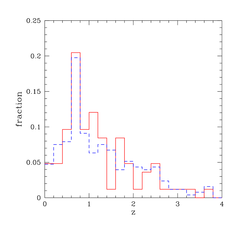
Figure 8: Normalized redshift distribution for the X–ray bright (solid line, 82 sources) and the X–ray faint (dashed line, 253 sources) subsamples.

We complete the analysis of the total sample fixing $\Gamma=1.8$ and deriving $N_{H}$ for the remaining faint sources (239/321). We remark that our division in a bright and a faint subsample does not correspond to a dramatic selection in redshift. Indeed, the X–ray bright and the X–ray faint subsamples have a similar distribution in redshift (see Figure 8). The results of the fits, along with the redshifts and the quality of the optical spectra, are shown in Table X–ray spectral properties of AGN in the Chandra Deep Field South.

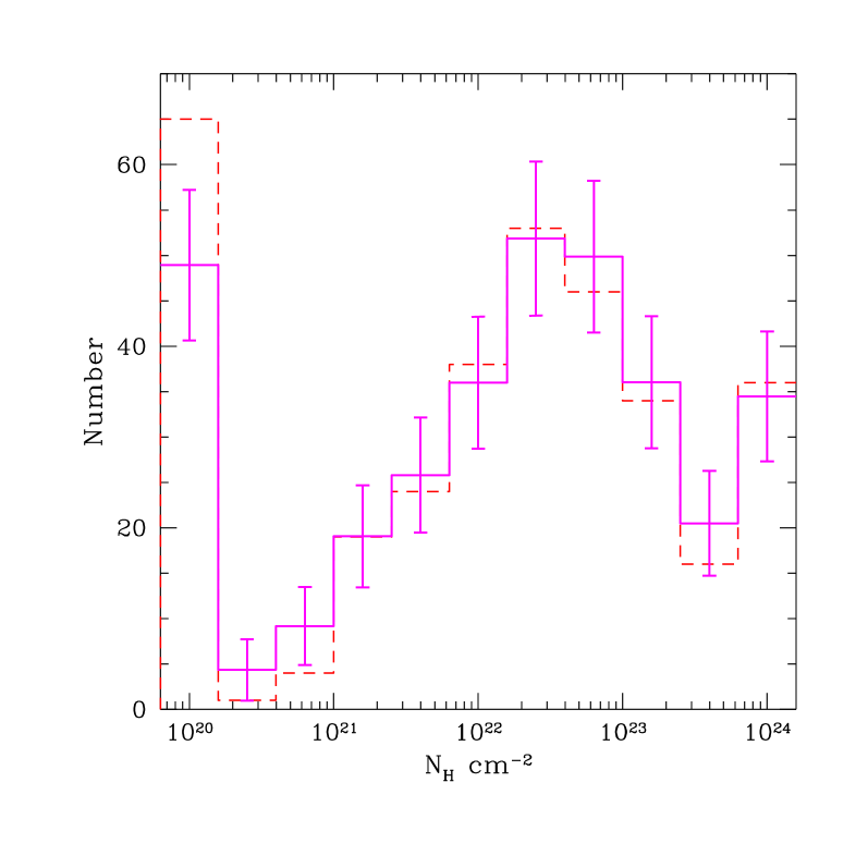
Figure 9: The solid line shows the observed $N_{H}$ distribution for the whole sample (321 sources). Error bars refer to 1$\sigma$ poissonian uncertainty due to the limited number of sources in each bin. The dashed histogram shows the distribution obtained without resampling according to measurement statistical errors. No correction for incompleteness and volume–sampling effects has been applied.

The distribution of the absorbing column densities is shown for the whole sample in Figure 9. Our results are in good agreement with preliminary results from the CDFN (Bauer et al. 2004a). The distribution has been obtained by extracting the value of $N_{H}$ of each source $10^{4}$ times from the range allowed by the statistical error bars, assuming gaussian errors. When the lower $\sigma$ error bars hit zero, we adopt the upper error bar to allow the $N_{H}$ resampled value to go below zero; in this case, the resampled values are included in the lowest bin. The lowest bin shown is the value of the Galactic absorption, $N_{H}\simeq 10^{20}$ cm^-2, below which we cannot measure the intrinsic absorption, especially at high redshifts. This bin includes all the sources with nominal $N_{H}$ best fit value lower than $10^{20}$ cm^-2. Among these sources we expect both redshifted AGN with low absorbing columns and normal X–ray galaxies. Note that here $N_{H}$ is an equivalent hydrogen column measured assuming the photo–electric cross–sections by Morrison & McCammon (1983), with metal abundances relative to Hydrogen by Anders & Ebihara (1982). The last bin at $N_{H}=10^{24}$ cm^-2 includes the few sources with measured $N_{H}>10^{24}$ cm^-2 and the Compton–thick candidates.

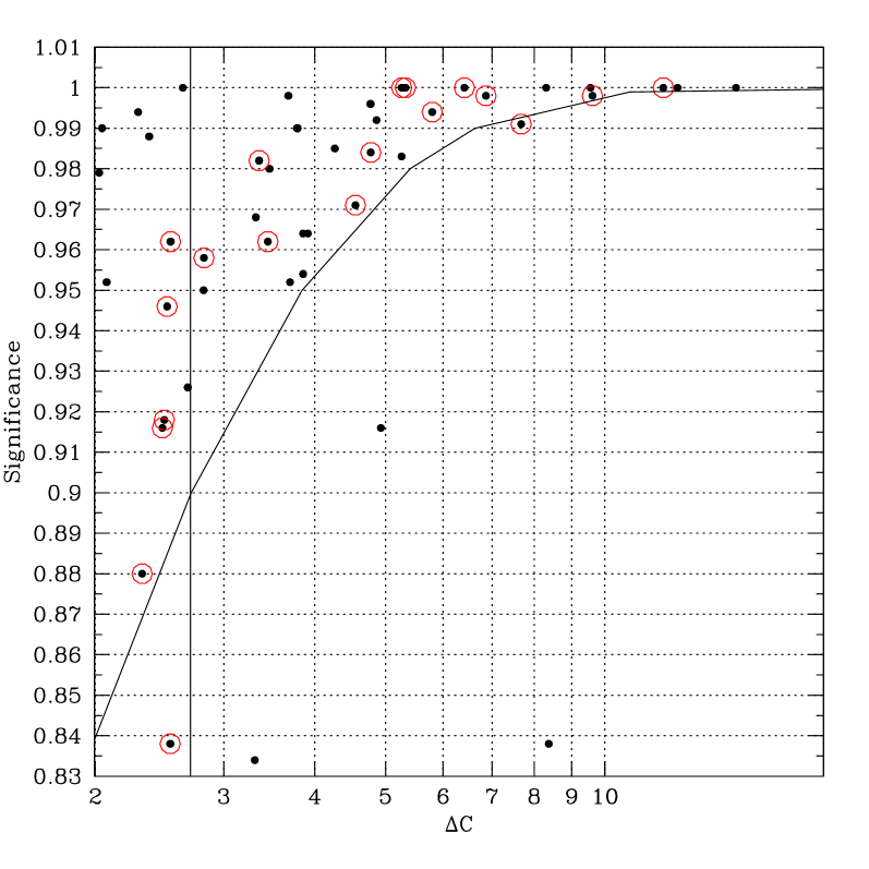
Figure 10: Significance of the Fe line (measured with simulations, see text) plotted versus the observed $\Delta C$. Pointed circles are sources included in the bright sample. The solid line shows the significance vs $\Delta C$ for one interesting parameter assuming the same statistics for $\Delta C$ and $\chi^{2}$. The vertical line is the threshold corresponding to $\Delta C=2.7$.

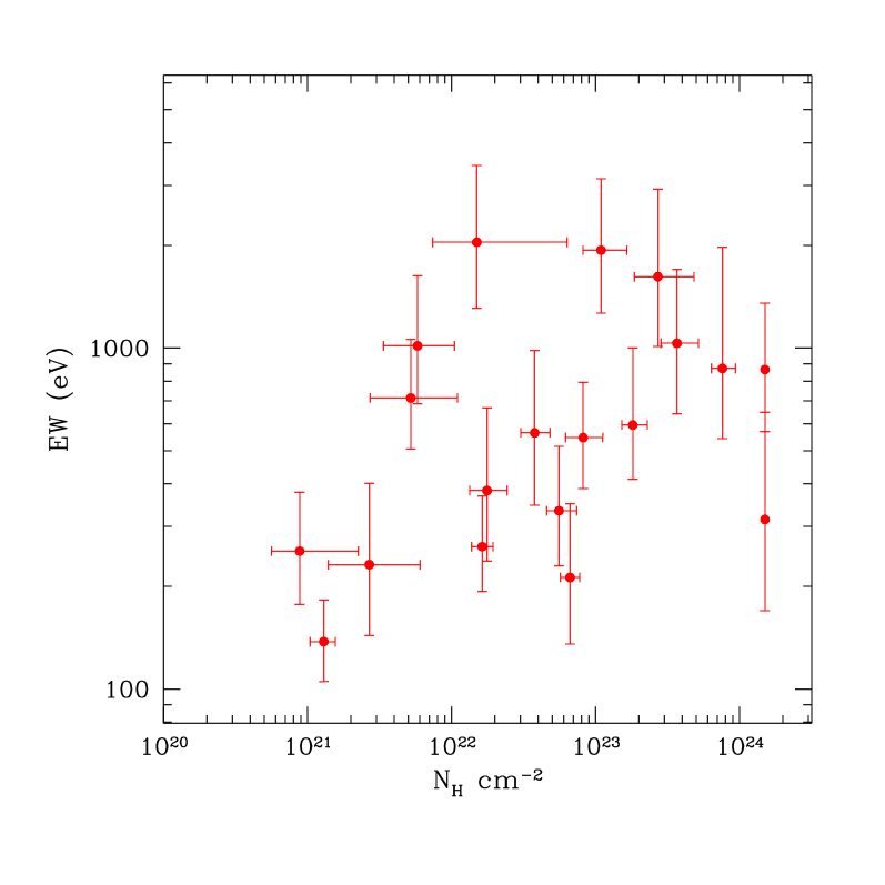
Figure 11: Equivalent width of the Fe line plotted versus the intrinsic absorption $N_{H}$ for the 20 sources with Fe line significant at more than 90% c.l. Errors on the equivalent width are derived from the errors on the normalization of the line component. Compton–thick candidates are plotted at $N_{H}=1.5\times 10^{24}$ as lower limits to the actual value.

We look for the Fe line only in those sources having at least 10 net counts in both bands, to have an acceptable estimate of the continuum and avoid spurious measures of high equivalent widths. Adopting a threshold $\Delta C\geq 2.7$ with respect to the fit without the line, corresponding to a minimum 90% c.l. for one interesting parameter, we find evidence for a significant Fe line in 20 sources with at least 10 net counts in both bands. The corresponding equivalent widths span the 100-3000 eV range. We carefully checked that our criterion $\Delta C>2.7$ actually corresponds to more than 90% c.l. also in the case of a line detection (for which the canonical confidence level criterion cannot be applied, see Protassov et al. 2002). For each X-ray source we simulated 500 spectra starting from the observed best fit model without the line. We then fitted each simulated spectrum and looked for any variation in the C-stat when adding a Fe line at $6.4/(1+z)$. The frequency of occurrence of $\Delta C_{sim}>\Delta C_{obs}$ gives the probability $P$ that the detected line is a statistical fluctuation. In Figure 10 we show the significance (1-$P$) of the Fe line versus the measured $\Delta C$. We conclude that in the large majority of the cases the criterion $\Delta C>2.7$ corresponds to a confidence level greater than 95%. Among the sources with more than 10 counts in both bands and a significant Fe line, 14/116 ($\sim 12$%) are found among the sources with spectroscopic redshift, and only 6/125 ($\sim 5$%) are found in the subsample with photometric redshift. This shows that, given our X–ray spectral resolution, the uncertainties in the photometric redshifts are likely to negatively affect the detection of the Fe line with our method, i.e., fixing the expected observing–frame energy of the line. Indeed, we notice that some sources do show strong hints of a Fe line at a redshift different from the photometric one (see Mainieri et al. 2005a), or peculiar lines (see Wang et al. 2003); finally, source variability could hide the emission line (see Braito et al. 2005). Therefore, we conclude that the fraction of sources with significant emission line is slightly larger than that found in an X–ray bright subsample in the CDFN (7%, see Bauer et al. 2004b). In principle, if the Fe line were produced only by the interaction of photons with the absorbing medium, a positive correlation between $N_{H}$ and equivalent width might be expected in obscured sources (Leahy & Creighton 1993; Ghisellini, Haardt & Matt 1994). As shown in Fig.11, we do not find strong evidence of a correlation given the scatter of our data points, as already observed (see Mushotzky, Done & Pounds 1993). The Fe lines measured with low intrinsic absorption ($N_{H}<10^{22}$ cm^-2), may be produced by the accretion disk, therefore breaking the expected correlation.

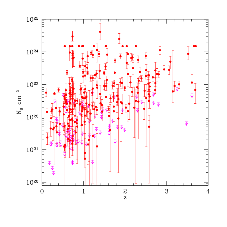
Figure 12: Intrinsic absorption versus redshift for the complete sample. Upper limits (1 $\sigma$) are used for measures consistent with $N_{H}=0$ within 1 $\sigma$. Compton–thick candidates are plotted at $N_{H}=1.5\times 10^{24}$ as lower limits to the actual value. Error bars correspond to 1 $\sigma$.

In figure 12 we show the scatter plot of intrinsic absorption as a function of redshift for the whole sample. We note the lack of sources with high absorption ($N_{H}>10^{22}$ cm^-2) at $z<1$. This is due to the fact that the low–luminosity, low–z sources with high absorption show a strongly suppressed flux, and only the intrinsically more luminous, rarer sources can be detected for a given threshold in count rate; the detection probability, then, decreases due to the small volume probed at low–z. We also note a lack of sources with low absorption (around $N_{H}\sim 10^{21}$ cm^-2) at high z. This effect may be due to the difficulty in measuring $N_{H}$ at $z>2$, since the absorption cutoff is redshifted below the lower limit of the Chandra energy band we use (0.6 keV). This effect could result in spuriously high values of $N_{H}$ with large error bars. Note, however, that some of the points are just 1 $\sigma$ upper limits, implying the presence of sources with low $N_{H}$ value at high redshift as well. It is clear that the $N_{H}$–$z$ scatter plot shows the effects of the incompleteness and partial sampling of the AGN population. Before investigating the shape and evolution of the intrinsic $N_{H}$ distribution, we must correct for the number of sources with a given $L_{X}$, $N_{H}$ and $z$ that fall outside our detection criteria. We will do this in the next Section.

In Figure 13 we show the scatter plot of $N_{H}$ versus the intrinsic, unabsorbed luminosities in the soft and in the hard band. We remark that the intrinsic luminosities are computed in the rest–frame soft and hard bands setting to zero the intrinsic absorption in the XSPEC best fit model; for the Compton–thick candidates we measure the intrinsic luminosities using a power law model with $\Gamma=1.8$ and normalization fixed to that of the best fit pexrav model. With this assumption the emitted (reflected) luminosity of the C–thick sources is always about 6% of the intrinsic one in the hard band (while only 0.2% in the soft). We also note that this model may give a lower limit to the intrinsic luminosity, since its assumes a maximally efficient reflection; the intrinsic luminosity can be higher for lower refelection efficiency (Ghisellini, Haardt & Matt 1994). The envelope at low luminosity and high $N_{H}$ is due to the fact that our survey is flux limited. The luminosity lower limit at a given redshift is not sharp, for two reasons: first, our survey is count–rate limited, and different spectral shapes may correspond to different fluxes and luminosities for the same count rates; second, the unabsorbed luminosities are related to the observed fluxes by a correction that depends on the measured $N_{H}$. For a preliminary investigation of a correlation between $N_{H}$ and intrinsic luminosity, we select two regions in Fig.13: i) $L_{X}>10^{43}$ erg s^-1 and $N_{H}<10^{24}$ cm^-2; ii) $L_{X}>10^{42}$ erg s^-1 and $N_{H}<10^{23}$ cm^-2. In this way we try to minimize the effects due to the flux–limited nature of our sample. In the first case, we do not find significant correlation between $N_{H}$ and hard luminosity (Spearmann Rank coefficient $SR=0.06$ for 154 sources). In the second case as well, we do not detect significant correlation between $N_{H}$ and hard luminosity (Spearmann Rank coefficient $SR=0.08$ from 184 sources). This result is not in disagreement with results obtained from larger samples. Indeed, in flux–limited samples, the dependence of the absorbed fraction on luminosity tends to be much weaker, as discussed by Perola et al. (2004). In the following, we will not introduce by hand the correlation between the absorbed fraction and luminosity found in larger sample spanning more than six decades in flux. The inability of retrieving in our sample such a correlation, will not affect our main results, like the intrinsic distribution of $N_{H}$, with the caveat that we are probing the luminosity range up to few $\times 10^{44}$ erg s^-1.

In Figure 13 we also show the locus of TypeII QSO, which is the upper right corner marked with the dashed lines. The criterion is $L_{X}>10^{44}$ erg s^-1 and $N_{H}>10^{22}$ cm^-2. For a spectral slope of $\Gamma=1.8$, a total luminosity of $10^{44}$ erg s^-1 in the 0.5-10 keV band corresponds to $3.9\times 10^{43}$ erg s^-1 in the 0.5–2 keV band and $6.1\times 10^{43}$ erg s^-1 in the 2–10 keV band. With these criteria, using X–ray spectral parameters and, most importantly, unabsorbed luminosities, the number of QSOII in the CDFS sample is 54. This corresponds to a surface density of X–ray selected QSO equal to $(620\pm 80)$ sq deg^-2 at the flux limit of $5\times 10^{-16}$ erg cm^-2 s^-1. This is higher than the value found by Padovani et al. (2004), but the difference is due to their selection based on the condition $L_{2-10}>10^{44}$ erg s^-1. Applying the same criteria, we find a surface density of $(360\pm 50)$ sq deg^-2 in very good agreement with Padovani et al. (2004; see also La Franca et al. 2005). We note, however, that the density of TypeII QSO depends sensitively on the luminosity cut in the intrinsic power used in the analysis.

Finally, we present a sample of 14 Compton–thick candidates selected only on the basis of the X–ray spectral shape with the selection thresholds described in §3.2. Two of them were already identified as Compton–thick sources on the basis of multiwavelength data (source ID 202 and 263, see Norman et al. 2002; Mainieri et al. 2005b). We assign a value $N_{H}\gtrsim 1.5\times 10^{24}$ cm^-2 to our Compton–thick candidates. Among them, 2 sources (out of 7 with secure spectroscopic redshift) show a Fe K emission line, while no Compton thick candidate source with photometric redshift does show a statistically significant line. We believe that the uncertainties in the photometric redshift prevent us from recovering the line. We also note that some high column density sources at low redshift may not have strong Fe K lines (see Fruscione et al. 2005). We checked that the distribution of the net detected counts of the C–thick candidates is not different from that of the whole sample, indicating that there are no evident bias due to the low signal–to–noise. The net–detected counts for the C–thick sample ranges from 170 to 40, with an average of 65. We notice that for these sources the detection probability is low, due to their hard spectra. Consequently, their associated sky–coverage is low, and their surface density correspondingly higher, close to $(200\pm 50)$ deg^-2. The actual surface density of C–thick sources may be 20% higher if including selection effects (see Appendix C). We notice also that the fraction of C–thick sources predicted by updated models for the synthesis of the XRB is in very good agreement with that found in the CDFS (Gilli, Comastri & Hasinger 2006, in preparation).

6 Intrinsic absorption distribution and its evolution with cosmic epoch

In this Section, we estimate the intrinsic absorption distribution (the $N_{H}$ function) for the AGN population in our sample. The distribution of $N_{H}$ that we showed in Figure 9, does not include any correction for incompleteness, and it refers only to the sources observed in the region of the $N_{H}$–$L_{X}$–$z$ space which is delimited by the count–rate detection thresholds of the survey. To go from this distribution to a distribution which is representative of the whole AGN population, we must apply two independent corrections. The first is the completeness correction and it is given by the effective solid angle under which a source of a given intrinsic luminosity, absorbing column density and redshift, is detected in the CDFS with our criteria. The second correction takes into account the sources which are outside the detectability region in the $N_{H}$–$L_{X}$–$z$ space, and therefore it must be based on a specific model of the luminosity function of AGN. We remind that a reliable luminosity function cannot be obtained from CDFS data alone, but should rather be derived from a combination of wider surveys, in order to sample the bright end of the luminosity distribution, which is poorly represented in our pencil beam survey (see Brandt & Hasinger 2005). We describe these two corrections below.

To correct for incompleteness, we simply weight each source for the inverse of the solid angle under which the source can be detected in the CDFS. To measure this quantity, first we compute the net count rate in the soft and hard band that would be measured in the aimpoint of the CDFS for each source in the sample, using its best–fit model. Then, we measure the solid angle $\omega_{i}$ where the $i$th source can be detected in the CDFS, including the vignetting correction and the background evaluated locally. Since the detection threshold is applied separately in the hard and the soft image, the effective solid angle is the largest between the two. We recall that our survey is limited in count rate, not in flux, and for a given intrinsic luminosity and redshift, the count rate is strongly dependent on the intrinsic absorption, especially in the soft band, where the sensitivity of our survey is the highest. Most of the sources have the largest detectability angle in the soft band, while the fewer, strongly absorbed, hard sources have the largest detectability solid angle in the hard image. The a priori probability of having a given source included in the CDFS sample is simply the ratio of the solid angle $\omega_{i}$ to the total solid angle covered by the 11 exposures of the CDFS ($\omega_{CDFS}=0.108$ deg²). Then, when binning our sample as a function of the measured $N_{H}$, we weight each source for the inverse of its detection probability:

$$F(N_{H})dN_{H}=\sum_{N_{H}bin}P_{i}\times(\omega_{i}/\omega_{CDFS})^{-1}\,.$$ (1)

Here, the weight $P_{i}$ would be equal to 1 if $N_{H}$ were measured with negligible error with respect to the size $dN_{H}$ of the bin. To account for statistical uncertainties in the measured value of $N_{H}$ for each source, we put $P_{i}$ equal to the probability that the actual value falls within the $N_{H}$ bin, according to the best fit value and its error bars. The error on $F(N_{H})$ is the poissonian error associated to the number of sources counted in the bin $N_{H}$–$N_{H}+dN_{H}$.

Then, we compute the second correction, to account for the sources which are outside the detectability region in the $N_{H}$–$L_{X}$–$z$ space in the CDFS survey. This correction is relevant for strongly absorbed sources, since our limit in count–rate allows us to sample a smaller range of intrinsic luminosity for increasing $N_{H}$ at a given redshift. This effect is mitigated at high redshift due to the positive X–ray K–correction. Therefore, for any given redshift and luminosity, we are measuring a different fraction of unabsorbed and absorbed sources with respect to the total AGN population. As a consequence, the directly observed fraction of sources with a given $N_{H}$ is affected by the shape of the actual AGN luminosity function and by its cosmic evolution.

To correct for this effect, we must assume a model for the AGN luminosity function. One of the most recent is the Luminosity Dependent Density Evolution model obtained by Ueda et al. (2003; but see Barger et al. 2005 for another determination of the AGN X–ray luminosity function consistent with pure luminosity evolution), in which low–luminosity sources peak at lower redshift than high–luminosity AGN. Such a luminosity function is measured from a combination of surveys with HEAO–1, ASCA and Chandra including part of the CDFN sample (see also Hasinger, Miyaji and Schmidt 2005 for the most recent measure of the Type I AGN luminosity function). In particular, we use equations 11-15-16-17 of Ueda et al. (2003) to write the comoving density of AGN per hard–band luminosity interval $N(L_{X},z)$.

After assuming a luminosity function for the whole AGN population, we can write the number of AGN in a given interval of $N_{H}$, $L_{X}$ and $z$ as

$$F(N_{H},L_{X},z)dN_{H}dL_{X}dz=N(L_{X},z)dL_{X}{{dV}\over{dz}}dz\,\,\,\,f(N_{H},L_{X},z)dN_{H}\,,$$ (2)

where $V$ is the comoving volume element, and $f(N_{H},L,z)$ is the probability of measuring an intrinsic absorption between $N_{H}$ and $N_{H}+dN_{H}$ for a given $L_{X}$ and $z$. Let’s assume that $f(N_{H},L,z)$ is slowly varying as a function of $L_{X}$ and $z$ in our sample. The total number of sources that we are detecting in our survey with intrinsic absorption between $N_{H}$ and $N_{H}+dN_{H}$ is then given by:

$$F(N_{H})dN_{H}=f(N_{H})dN_{H}\int^{z_{max}}_{0}{{dV}\over{dz}}dz\int^{L_{max}}_{L_{cut}(N_{H},z)}N(L_{X},z)dL_{X}\,\,$$ (3)

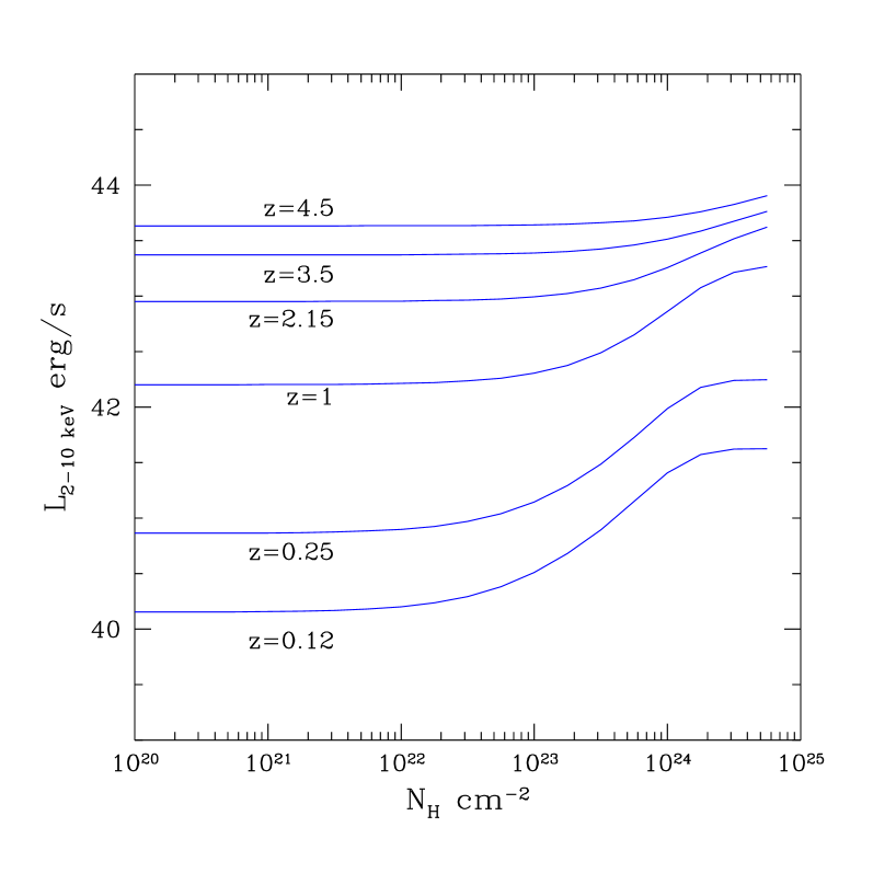
Figure 14: Intrinsic minimum rest–frame luminosity in the 2–10 keV band ($L_{cut}$) of a source that can be detected at the CDFS aimpoint as a function of intrinsic absorption for redshifts $z=0.12-0.25-1-2.15-3.5-4.5$ from the bottom to the top. The assumed model is a Compton thin power law with $\Gamma=1.8$ plus a reflection component equal to 6% of the hard intrinsic luminosity.

Here the luminosity $L_{cut}(N_{H},z)$ is the 2–10 keV intrinsic luminosity for which, at any given z and $N_{H}$, the net count rate is equal to the minimal count rates in the hard or in the soft band. The minimal count rates for detection in the aimpoint of the CDFS are $1.2\times 10^{-5}$ cts/s in the soft and $1.5\times 10^{-5}$ cts/s in the hard band. These values are defined with small uncertainties because of the rapid drop of the sky coverage as a function of the count rate in both bands. To compute $L_{cut}$, we assume that in average our sources can be described with a Compton–thin model with spectral slope fixed to $\Gamma=1.8$, plus a reflection component with the same slope and normalization. The reflection component (modeled with the pexrav XSPEC model) amounts to 6% of the hard intrinsic luminosity. Such a reflection component will dominate the emission of the Compton–thick sources with $N_{H}\geq 1.5\times 10^{24}$ cm^-2. The value of $L_{cut}$ as a function of $N_{H}$ is shown in Figure 14 for different redshifts. We note that for unabsorbed sources ($N_{H}<10^{22}$ cm^-2) the cut depends only on the intrinsic luminosity at any redshift. However, for larger column densities, the cut in luminosity is higher for larger $N_{H}$, but the effect is weaker at higher $z$ where the positive X–ray K–correction shifts the hard rest–frame emission in the soft band. In the Compton–thick regime, a roughly constant fraction of the intrinsic luminosity reflection by cold material dominates the emission, making $L_{cut}$ flat again. We do not attempt to include the effect of the presence of the scattered component, which is detected only in less than 3% of the sources in our sample.

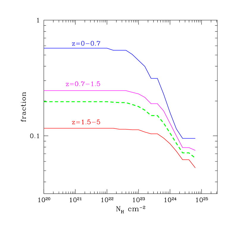
Figure 15: Total fraction of all the AGN detected in the CDFS survey as a function of the intrinsic $N_{H}$, according to the detection criteria in the CDFS and assuming the luminosity function of Ueda et al. (2003). The total fraction strongly depends on the minimum detectable luminosity and hence, given the flux limit in the CDFS, on the redshift range. Note that low fractions are implied by the conservatively low value $L_{min}$ ($10^{41}$ ergs s^-1) which defines the total population of AGN. The thick, dashed line is the correction for the whole sample. The three continuous lines refer to three intervals in redshifts: $z=0-0.7$, $z=0.7-1.5$, $z=1.5-5$ from top to bottom.

Since $F(N_{H})$ (computed with equation 1) is the directly observed $N_{H}$ distribution (after correcting for incompleteness), the probability function $f(N_{H})$ can be obtained after equation 3 (discretizing the integral over $N_{H}$). The resulting fraction of AGN visible in the CDFS as a function of $N_{H}$ is shown in Figure 15 for three different redshift intervals (solid lines), and for the whole explored redshift range (thick dashed line). This fraction is computed as the ratio of the detectable AGN over the total number of AGN predicted by the Ueda et al. luminosity function in the range $L_{max}=10^{45}$ ergs s^-1, $L_{min}=10^{41}$ ergs s^-1, and $z_{max}=5$. Note that the low values of this fraction does not imply that the majority of the AGN are not detected in the CDFS; in fact, such low values are mostly due to the conservatively low minimum luminosity adopted here ($L_{min}=10^{41}$ ergs s^-1) and depend on the faint end slope of the luminosity function. These aspects, in turn, weakly affects the dependence of the fraction on $N_{H}$, which is our main concern here. Here we do not discuss the effects of the shape of the underlying luminosity function, postponing this to a subsequent paper. Therefore, we estimate in a robust way the dependence of the total fraction of visible AGN on the redshift (given the flux limit in the CDFS) and on $N_{H}$. The fraction decreases towards higher values of $N_{H}$ due to the reduced emission in the soft band, but it flattens again in the Compton–thick regime, where the emitted luminosity is roughly a constant fraction of the intrinsic one.

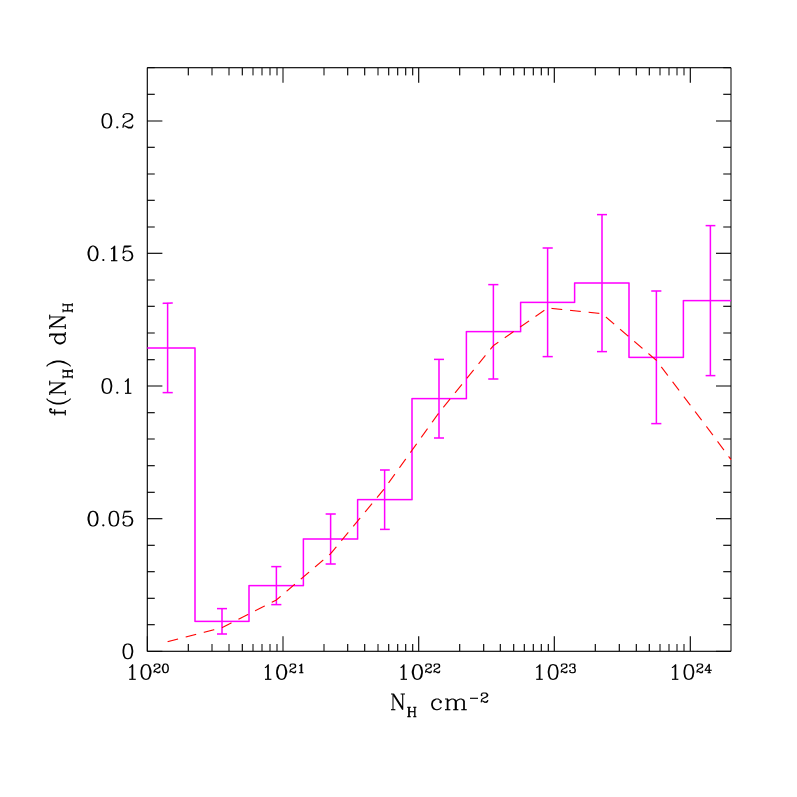
Figure 16: Intrinsic $N_{H}$ distribution representative of the whole AGN population in our sample (corrected for incompleteness and sampling–volume effect, and convolved with the statistical errors of each measurement). Errors are obtained from the poissonian uncertainties on the number of detected sources in each bin. The dashed curve is a lognormal distribution with $\langle log(N_{H})\rangle=23.1$ and $\sigma=1.1$. Compton–thick candidates are all in the bin at $N_{H}=10^{24}$.

The corrected, normalized distribution of the intrinsic absorption for the whole sample is shown in Figure 16. Errors are obtained from the poissonian uncertainties on the number of detected sources in each bin. The distribution that we measured is bimodal, in the sense that 10% of sources have $N_{H}<10^{20}$ cm^-2 and appear separated from the distribution of the bulk of the sources. However, we remark that the fraction of sources with negligible absorption in our sample may include normal galaxies with high star formation rate. The distribution of the bulk of the sources can be roughly approximated with a lognormal distribution centered on $\langle log(N_{H})\rangle\simeq 23.1$ and with a dispersion $\sigma=1.1$. We remark that in the Compton–thin regime, where our estimates are more robust, the number of obscured sources is steeply increasing with $N_{H}$ in agreement with Risaliti et al. (1999) and Dwelly et al. (2005).

This distribution accounts for the Compton–thin sources with intrinsic absorption up to $N_{H}\simeq 10^{24}$ cm^-2, and for Compton–thick sources at higher absorption, bridging the bulk of the AGN to the Compton–thick population. This is the main difference with the distribution presented in Treister et al. (2004), where the fraction of sources with $N_{H}>10^{23}$ cm^-2 is dropping. Indeed, strongly absorbed AGN are expected to be missed by surveys that rely on optical spectroscopy. Here we show that part of the population of Compton–thick sources can be detected in present deep X–ray Surveys via a careful spectral analysis of all the X–ray detected sources, avoiding selection based on optical spectroscopy. Our results are consistent with the preliminary results on the $N_{H}$ distribution found in the CDFN (Bauer et al. 2004a), which already shows a peak at larger $N_{H}$ values with respect to the results of Ueda et al. (2003). We remark that this result is not affected by small variations with respect to the luminosity function proposed by Ueda et al. (2003), which indeed is consistent with the present data on the AGN luminosity distribution. To summarize, we conclude that at least part of the expected population of strongly absorbed AGN (expected to be observed in the submillimiter with the Spitzer satellite) is already present in the deep X–ray Survey such as the CDFS.

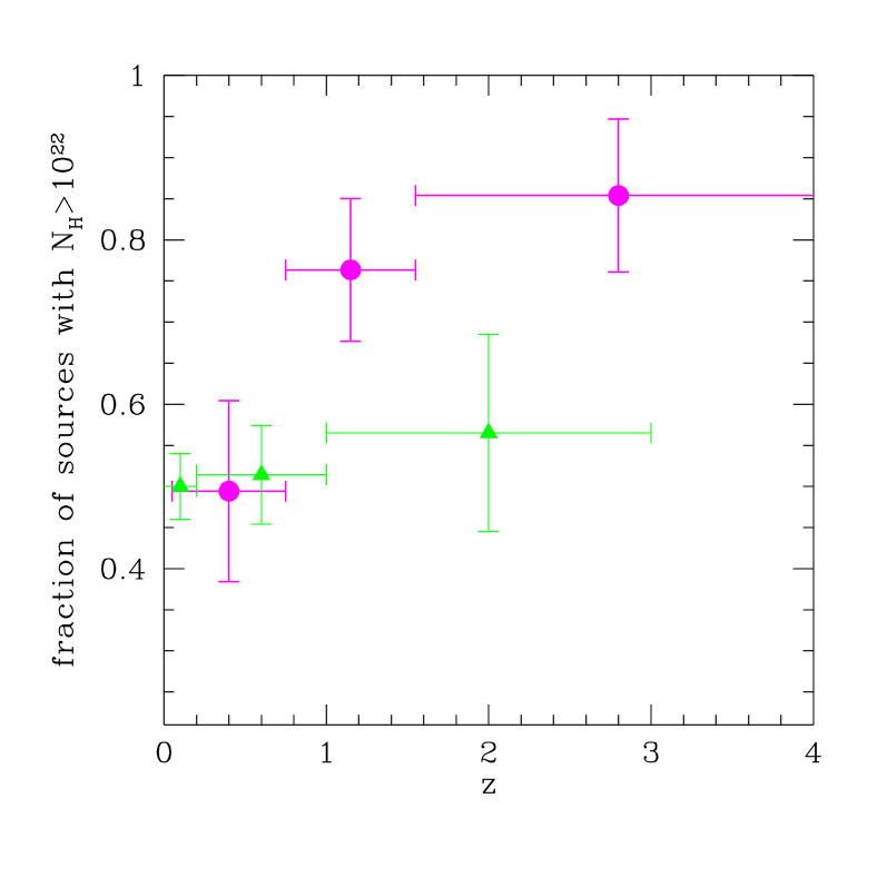
Figure 17: Fraction of absorbed AGNs with $N_{H}>10^{22}$ cm^-2 to all AGNs with $L_{X}>10^{41}$ erg s^-1 (2–10 keV band) as a function of redshift (solid circles). Triangles are the data points from Ueda et al. (2003) for $10^{43}<L_{X}<10^{44.5}$ erg s^-1 (2–10 keV band). Rest–frame luminosities are computed for a $\Lambda=0.7$ flat cosmology and $H_{0}=70$ km/s/Mpc.

The $N_{H}$ function is derived under the assumption of no strong intrinsic correlation between $L$ and $N_{H}$ or $z$ and $N_{H}$ in our sample, so that we can obtain $f(N_{H})$ without binning our sample as a function of $L_{X}$ or $z$. However, here we investigate for possible evolution with redshift of the absorbed fraction of sources. Due to the limited statistics, we focus on the cosmic evolution of the ratio of absorbed sources ($N_{H}>10^{22}$ cm^-2) to all the AGNs in three bins of redshift. The redshift bins are $z=0-0.7$, $0.7-1.5$, $1.5-5$, including 76, 125 and 109 sources with $L_{X}>10^{41}$ erg s^-1 respectively (the first two bins include the two most prominent spikes in the CDFS redshift distribution at $z=0.67$ and $z=0.73$, as shown in Gilli et a. 2003). The correction for the absorbed sources that are missed is larger at low redshift, as can be seen in Figure 15 (upper curve for the redshift range $z=0$–$0.7$), while at high z is almost flat up to log($N_{H}$)$=23.5$ (lower curve for the redshift range $z=1.5$–$5$). In Figure 17 we show that the absorbed fraction is consistent with a moderate increase, in agreement with the model of Gilli et al. (2001; see also Civano, Comastri & Brusa 2005). We remark that the absorbed fraction in the first bin at $z<0.8$, including the low luminosity sources, may be underestimated due to the presence of star forming galaxies in the luminosity range $10^{41}$–$10^{42}$ erg s^-1.

We note that the overall value of the fraction of absorbed sources is larger than that found by Ueda et al. (2003). However, the points of Ueda et al. (2003) include only sources with $L_{X}>10^{43}$ erg s^-1, and therefore are expected to be significantly higher when including lower luminosities. The global fraction of absorbed sources is in agreement with that estimated in the CDFN by Perola et al. (2004), and with a ratio of absorbed over unabsorbed sources in the sample of about 4, as observed in the local Universe (eg. Maiolino & Rieke 1995). This value is also consistent with the theoretical expectation of 3/4 of all the AGN being absorbed as in the standard unification scenario (Antonucci 1993). While in the CDFS and CDFN the fraction of obscured sources seems to be in agreement with the expectations of the standard unification scenario and popular synthesis models of the X–ray background, in shallower serendipitous surveys like those performed with XMM by Piconcelli et al. (2003) and Mateos et al. (2005) obscured sources seem to be a factor of $\simeq 2$ less abundant. At typical X–ray fluxes of a few $10^{-14}$ erg s^-1 cm^-2, XMM serendipitous sources have a median luminosity of a few $10^{44}$ erg s^-1. It is therefore possible that the intrinsic fraction of obscured sources is decreasing at luminosities higher than that observed in the Chandra Msec fields, which would point towards a paucity of obscured QSOs as found by Ueda et al. (2003; see also La Franca et al. 2005). Alternatively, one could argue about the large spectroscopic incompleteness of XMM samples (more than 60% of the sources are as yet unidentified) before drawing solid conclusions.

7 Comparison between X–ray and Optical properties

If we classify the whole sample of 321 sources with $L_{X}>10^{41}$ erg s^-1, according only to the optical spectra, we obtain the following:

• 34 Broad Line AGN (BLAGN);

• 20 High Excitation Line galaxies (HEX);

• 67 Low Excitation Line Galaxies (LEX);

• 22 Absorption spectrum typical of late–type galaxies;

• 178 non classified.

In this section we compare the optical classification with the X–ray classification, to investigate if a revision of the unification model is actually needed (see, e.g., Matt 2002). This was already done in Szokoly et al (2004); the main difference here is that we use unabsorbed luminosities and intrinsic absorption as opposed to absorbed luminosities and hardness ratio, providing therefore a more physical X–ray classification. We use the value $N_{H}=10^{22}$ cm^-2 as the threshold to divide X–ray unabsorbed sources from X–ray absorbed ones. We define normal X–ray galaxies the sources with $N_{H}<10^{22}$ cm^-2 and $L_{X}<10^{42}$ erg s^-1. Our results are shown in Table X–ray spectral properties of AGN in the Chandra Deep Field South, to be compared with Table 8 of Szokoly et al. (2004). We remark that the class “normal galaxies”, amounting to 42 sources, may include low luminosity AGN. Indeed, if we restrict our criterion to source with low intrinsic absorption (values $N_{H}<10^{21}$ cm^-2 can be due also to diffuse matter in the host galaxy, as opposed to the larger absorbing columns typical of circumnuclear matter), the normal galaxies class would include 23 sources only. Therefore, we can bracket the contamination of our sample by normal galaxies to be between 7% and 14% of the total sample.

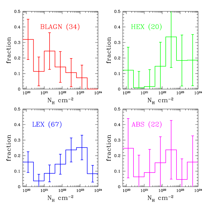
Figure 18: Normalized $N_{H}$ distribution for the four different optical classes (see text).

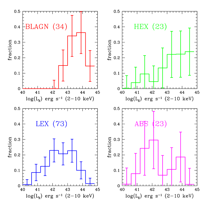
Figure 19: Normalized distribution of the intrinsic rest–frame luminosity in the hard band for the four different optical classes (see text).

We also plot the normalized distribution of the intrinsic absorption and hard luminosities for the four optical classes in Figures 18 and 19. Here we account for the statistical errors by resampling each value according to its error bars, but we do not introduce any correction for selection effects, since here we are dominated by optical selection criteria. We find that, as expected, the BLAGN class mostly includes AGN with low absorbing column densities: among the 34 BLAGN, only 7 sources have $N_{H}>10^{22}$ cm^-2; they give a fraction of 0.18 of BLAGN with $N_{H}>10^{22}$ cm^-2, after accounting for statistical errors. This fraction is somewhat larger than that found in shallower surveys by Perola et al. (2004) and in the ChaMP survey by Silverman et al. (2005). However, we notice that most of the absorbed BLAGN are at $z\geq 2$. Due to the large errors expected when measuring $N_{H}$ in high redshift sources, we do expect a scatter towards high values increasing with redshift. A spurious trend $N_{H}\propto(1+z)^{3}$ may be visible if we simply plot the best fit values for $N_{H}$. We carefully checked with simulations with XSPEC that the error bars keep track of this effect, being larger at higher z. In these simulations, described in Appendix C, we show that in the hypothesis of $N_{H}\simeq 0$ for all the BLAGN sources, we should expect none of them to have $N_{H}>0$ at 2 $\sigma$ c.l. Instead, we find five of them to have $N_{H}>10^{22}$ cm^-2 at 2 $\sigma$. Using the better count statistics and the larger energy range ($E>0.2$ keV) of XMM (see Streblyanska et al. 2004), the spectral analysis of 5 of these sources gives absorption in the range $10^{21}<N_{H}<10^{22}$ cm^-2, confirming that these BLAGN have a non–negligible absorption, but that the Chandra best–fit values are somewhat higher, possibly due to the limited energy range used which may hamper the measure of low column densities at high z. To summarize, we put a strict upper limit of 18% for absorbed sources ($N_{H}>10^{22}$ cm^-2) within BLAGN.

Absorbed AGNs with $N_{H}>10^{22}$ cm^-2 are found mostly in the HEX and LEX classes (80% and 60% respectively). They are also found in the ABS class, where, however few sources have $N_{H}>10^{22}$ cm^-2. We find less evidence for Narrow Line AGN (here classified as HEX) with low absorption. We observe only about $\sim 10$% of such sources, for which the most likely scenario is severe dilution of the AGN optical emission by the underlying galaxy. Therefore, the simple identification scheme of unabsorbed AGN with optical Type I (BLAGN) and absorbed AGN with optical Type II (HEX and LEX) is roughly correct, with uncertainties of less than 20%.

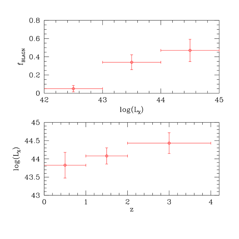
Figure 20: Upper panel: fraction of BLAGN among the sample of sources with optical redshift as a function of the 0.5-10 keV luminosity bin. Lower panel: average 0.5-10 keV luminosity of BLAGN as a function of the redshift bin. Only sources with $L_{X}>10^{43}$ erg s^-1 are considered in the lower panel.

As for the hard luminosities (Figures 19), we show that the BLAGN and HEX classes have X–ray luminosities in the range $10^{42}$–$10^{44}$ erg s^-1 typical of AGN, with very few sources below $10^{42}$ erg s^-1. The value $10^{42}$ erg s^-1 can be considered as an effective luminosity threshold dividing AGN and normal or star forming galaxies, except for few cases of galaxies with a strong starburst, which can reach $L_{X}\sim 10^{42}$ ergs s^-1 for a star formation rate of about 100 $M_{\odot}/yr$ (Ranalli et al. 2003). This luminosity range, where the presence of normal galaxies is expected to be significant, starts to be progressively populated in the LEX and ABS classes. However, also for the HEX class the majority of the sources have luminosities $L_{X}>10^{42}$ erg s^-1, and only the ABS class is consistent with being an equal mix of galaxies and AGN. The distribution of the intrinsic rest–frame luminosities in the hard bands shows that broad line AGN have larger intrinsic luminosities than narrow line AGN, as noted by Barger et al. (2005). In particular, the fraction of BLAGN in our sample among the sources with optical spectra, is strongly increasing with luminosity, while their average luminosity is increasing with redshift, in agreement with the findings of Steffen et al. (2003), as shown in Figure 20. However, due to our small sampling volume at low redshift, to the low optical spectral completeness of our sample ($\simeq 1/3$), and, finally, to the possible effect of the stellar dilution that may hinder the presence of broad lines (see, e.g., Moran et al. 2002) we do not draw strong conclusion on this aspect.

We note also that, given the intrinsic luminosities and the intrinsic absorption values found in the remaining subsample of 178 sources without a clear optical classifications, about 90% of them are expected to be secure AGN. Overall, we find that at least 80% of the AGN with spectral ID in our sample agrees with simple AGN unification models (Antonucci 1993), confirming findings of wider and shallower surveys (see, e.g., Silverman et al. 2005).

8 Conclusions

We presented the detailed spectral analysis of 321 sources in the CDFS, taking advantage of spectroscopic and photometric redshifts. We fitted the source X–ray spectra assuming a default model consisting in a single power law with intrinsic redshifted absorption (plus a local absorption frozen to the Galactic value in the direction of the CDFS) and a Gaussian line at the redshifted energy of the Fe K line complex. We look for sources with a spectrum dominated by a reflection component (Compton–thick candidates) and for sources showing an unabsorbed scattered component at soft energies. We are able to derive the spectral slope distribution for the 82 brightest sources in the sample and intrinsic absorbing column density for the whole sample. Then, from the observed $N_{H}$ distribution, we derive the intrinsic $N_{H}$ distribution for the whole AGN population, after correcting for incompleteness and for the differential sampling of the AGN population as a function of intrinsic luminosity and $N_{H}$ (modelling the luminosity function of AGN after Ueda et al. 2003). We accounted for statistical errors in our measures by convolving the distributions according to the error bars associated to each measurement. We also look for evolution in the fraction of absorbed sources as a function of the redshift. Our main results are summarized as follows:

• We investigate the spectral slope of the intrinsic spectrum for the 82 sources of the X–ray bright sample, excluding the two brightest that otherwise would dominate the statistics. We find that the average value for the slope of the power law is $\langle\Gamma\rangle\simeq 1.75\pm 0.02$, with an intrinsic dispersion of the order of $\sigma_{int}\simeq 0.30$.

• We find no correlation between the spectral index $\Gamma$ and the intrinsic absorption column density $N_{H}$ nor the intrinsic luminosity. We do not detect any evolution of the average $\Gamma$ with redshift.

• We select 14 Compton–thick candidates, for which we can only assess a lower limit to the intrinsic column density of $N_{H}>1.5\times 10^{24}$ cm^-2. Due to their low detectability, the surface density can be as high as $(200\pm 50)$ deg^-2.

• We find significant evidence (at more than 90% confidence level) of a Fe line in 20 sources, most of them (14) for the sources with spectroscopic redshifts. We also find unabsorbed soft emission, fit with a power law model with the same slope as the main power law, possibly associated with a scattered component, in only 8 sources.

• The intrinsic $N_{H}$ distribution is well approximated by a lognormal distribution centered on $\langle log(N_{H})\rangle\simeq 23.1$ and with a dispersion $\sigma=1.1$. This distribution differs from that found by Ueda et al. (2003), which shows a broader peak at lower values of $N_{H}$. Our distribution includes the contribution of many more absorbed AGN, since we explored the faint X–ray flux range, where strongly absorbed sources dominate in number. This shows that the population of Compton–thick AGN (expected to be observed with the Spitzer satellite) is at least partly accounted for in deep X–ray surveys when all the X–ray selected sources are included.

• We find hints that the fraction of absorbed sources is increasing with redshift, consistently with XRB synthesis models.

• We find that the simple unification model, i.e. the one–to–one correspondence of unabsorbed/absorbed X–ray sources to TypeI AGN–QSO/TypeII AGN–QSOII, is accurate for at least 80% of the sources with spectral identification ($\sim 1/3$ of the total X-ray sample).

We remark that once the ongoing or planned spectroscopic follow–up of the many Chandra and XMM surveys will be completed, the same kind of detailed spectral analysis will be performed on a much larger number of sources. This will allow one to firmly understand the distribution of spectral properties among AGN, and to suggest improvements to the unification model in view of the complex relation between X–ray and optical types.

[x]llllllllll Best fit parameters for the whole sample of sources in the CDFS with a measured spectroscopic or photometric redshift. Error bars correspond to 1 $\sigma$ c.l. Luminosities are computed for a flat $\Lambda=0.7$ cosmology and $H_{0}=70$ km/s/Mpc. ID are from Giacconi et al. (2002). Quality flags with $Q\geq 1$ indicate optical spectral quality: $Q=1$ corresponds to spectra with a single optical line identified; $Q=2$ indicates secure spectra but uncertain counterpart; $Q=3$ indicates secure redshift. Photometric redshifts are obtained from different methods described in Zheng et al. (2004): HyperZ ($Q=0.2$), BPZ ($Q=0.3$), COMBO–17 ($Q=0.4$ Wolf et al. 2001; 2003; 2004). When we have consistent redshift from more than one method, the corresponding quality flag is the sum of the single $Q$.
ID z Q $\Gamma$ $N_{H}/10^{22}$ cm^-2 $L_{soft}$ erg s^-1 $L_{hard}$ erg s^-1 $F_{0.5-2}$ cgs $F_{2-10}$ cgs X–type

1 0.347 1.6 $1.54_{-0.21}^{+0.17}$ $0.52_{-0.14}^{+0.16}$ $7.57\times 10^{41}$ $1.73\times 10^{42}$ $1.20\times 10^{-15}$ $4.78\times 10^{-15}$ C–thin
2 0.730 0.4 $3.04_{-0.23}^{+0.31}$ $1.43_{-0.18}^{+0.27}$ $4.37\times 10^{43}$ $9.54\times 10^{42}$ $2.72\times 10^{-15}$ $2.19\times 10^{-15}$ C–thin
3 0.220 0.4 $1.80$ $0.91_{-0.21}^{+0.22}$ $2.68\times 10^{41}$ $4.19\times 10^{41}$ $6.65\times 10^{-16}$ $2.91\times 10^{-15}$ C–thin
4 1.260 1.0 $1.68_{-0.08}^{+0.14}$ $0.00^{+0.29}$ $2.36\times 10^{43}$ $4.37\times 10^{43}$ $3.28\times 10^{-15}$ $6.12\times 10^{-15}$ C–thin
6 2.460 0.2 $1.91_{-0.12}^{+0.13}$ $1.80_{-0.95}^{+0.96}$ $2.09\times 10^{44}$ $2.73\times 10^{44}$ $3.79\times 10^{-15}$ $6.40\times 10^{-15}$ C–thin
7 1.840 0.6 $2.16_{-0.16}^{+0.21}$ $3.57_{-0.63}^{+0.91}$ $4.55\times 10^{44}$ $4.36\times 10^{44}$ $7.98\times 10^{-15}$ $1.55\times 10^{-14}$ C–thin
8 0.990 0.9 $1.80$ $3.77_{-0.49}^{+0.64}$ $2.45\times 10^{43}$ $3.74\times 10^{43}$ $1.61\times 10^{-15}$ $7.95\times 10^{-15}$ C–thin
9 1.990 0.4 $1.80$ $0.00^{+0.46}$ $1.45\times 10^{44}$ $2.25\times 10^{44}$ $6.33\times 10^{-15}$ $9.89\times 10^{-15}$ C–thin
10 0.424 3.0 $1.17_{-0.20}^{+0.22}$ $1.51_{-0.42}^{+0.48}$ $1.13\times 10^{42}$ $4.55\times 10^{42}$ $8.68\times 10^{-16}$ $8.96\times 10^{-15}$ C–thin
11 2.579 3.0 $1.79_{-0.09}^{+0.09}$ $0.51_{-0.50}^{+0.63}$ $2.92\times 10^{44}$ $4.52\times 10^{44}$ $6.56\times 10^{-15}$ $1.11\times 10^{-14}$ C–thin
12 0.251 3.0 $1.91_{-0.10}^{+0.10}$ $0.00^{+0.03}$ $5.38\times 10^{41}$ $7.24\times 10^{41}$ $2.86\times 10^{-15}$ $3.84\times 10^{-15}$ C–thin
13 0.733 3.0 $1.72_{-0.08}^{+0.09}$ $0.00^{+0.05}$ $1.11\times 10^{43}$ $1.91\times 10^{43}$ $5.16\times 10^{-15}$ $9.16\times 10^{-15}$ C–thin
15 1.227 1.0 $1.74_{-0.14}^{+0.14}$ $0.26_{-0.25}^{+0.33}$ $2.27\times 10^{43}$ $3.95\times 10^{43}$ $2.86\times 10^{-15}$ $5.58\times 10^{-15}$ C–thin
17 0.870 0.6 $1.56_{-0.09}^{+0.16}$ $0.00^{+0.20}$ $2.43\times 10^{42}$ $5.33\times 10^{42}$ $8.45\times 10^{-16}$ $1.88\times 10^{-15}$ C–thin
18 0.979 3.0 $1.74_{-0.08}^{+0.04}$ $1.91_{-0.22}^{+0.19}$ $6.69\times 10^{43}$ $1.13\times 10^{44}$ $7.30\times 10^{-15}$ $2.63\times 10^{-14}$ C–thin
19 0.740 3.0 $1.87_{-0.13}^{+0.15}$ $0.26_{-0.17}^{+0.16}$ $2.11\times 10^{43}$ $2.88\times 10^{43}$ $7.06\times 10^{-15}$ $1.24\times 10^{-14}$ C–thin
20 1.016 3.0 $1.78_{-0.27}^{+0.28}$ $5.64_{-1.26}^{+1.44}$ $1.16\times 10^{43}$ $1.86\times 10^{43}$ $5.43\times 10^{-16}$ $3.66\times 10^{-15}$ C–thin
21 3.476 3.0 $1.80$ $0.00^{+0.72}$ $4.56\times 10^{43}$ $6.85\times 10^{43}$ $5.53\times 10^{-16}$ $8.65\times 10^{-16}$ C–thin
22 1.920 3.0 $1.79_{-0.07}^{+0.12}$ $0.02_{-0.02}^{+0.54}$ $7.69\times 10^{43}$ $1.21\times 10^{44}$ $3.66\times 10^{-15}$ $5.87\times 10^{-15}$ C–thin
23 0.730 0.5 $1.98_{-0.21}^{+0.23}$ $0.15_{-0.09}^{+0.27}$ $4.80\times 10^{42}$ $5.64\times 10^{42}$ $1.65\times 10^{-15}$ $2.36\times 10^{-15}$ C–thin
24 3.610 3.0 $1.56_{-0.17}^{+0.17}$ $1.99_{-2.02}^{+3.20}$ $1.10\times 10^{44}$ $2.39\times 10^{44}$ $1.58\times 10^{-15}$ $4.01\times 10^{-15}$ C–thin
25 2.260 0.5 $0.29_{-0.20}^{+0.21}$ $3.17_{-3.17}^{4.05}$ $3.85\times 10^{42}$ $6.36\times 10^{43}$ $5.84\times 10^{-16}$ $1.19\times 10^{-14}$ C–thin
26 1.650 0.5 $1.80$ $3.77_{-0.95}^{+1.05}$ $2.44\times 10^{43}$ $3.98\times 10^{43}$ $7.69\times 10^{-16}$ $2.58\times 10^{-15}$ C–thin
27 3.064 3.0 $1.22_{-0.25}^{+0.26}$ $28.08_{-7.97}^{+9.18}$ $5.23\times 10^{43}$ $2.13\times 10^{44}$ $6.85\times 10^{-16}$ $6.95\times 10^{-15}$ C–thin
28 1.216 3.0 $1.80$ $2.21_{-0.55}^{+0.58}$ $1.11\times 10^{43}$ $1.75\times 10^{43}$ $7.44\times 10^{-16}$ $2.36\times 10^{-15}$ C–thin
29 0.300 0.9 $2.02_{-0.19}^{+0.14}$ $5.32_{-0.42}^{+0.53}$ $8.71\times 10^{42}$ $9.66\times 10^{42}$ $2.14\times 10^{-15}$ $2.63\times 10^{-14}$ Soft–C
30 0.837 3.0 $1.68_{-0.10}^{+0.17}$ $0.00^{+0.19}$ $3.80\times 10^{43}$ $6.99\times 10^{43}$ $1.33\times 10^{-14}$ $2.52\times 10^{-14}$ C–thin
31 1.603 3.0 $2.12_{-0.09}^{+0.09}$ $1.79_{-0.18}^{+0.36}$ $1.75\times 10^{44}$ $1.66\times 10^{44}$ $5.57\times 10^{-15}$ $8.76\times 10^{-15}$ C–thin
32 0.664 3.0 $1.87_{-0.14}^{+0.38}$ $0.13_{-0.15}^{+0.19}$ $4.57\times 10^{42}$ $6.52\times 10^{42}$ $2.16\times 10^{-15}$ $3.63\times 10^{-15}$ C–thin
33 0.665 3.0 $1.59_{-0.10}^{+0.11}$ $0.19_{-0.14}^{+0.14}$ $7.38\times 10^{42}$ $1.55\times 10^{43}$ $3.93\times 10^{-15}$ $9.86\times 10^{-15}$ C–thin
34 0.839 3.0 $1.58_{-0.18}^{+0.21}$ $0.64_{-0.32}^{+0.37}$ $5.20\times 10^{42}$ $1.10\times 10^{43}$ $1.33\times 10^{-15}$ $4.15\times 10^{-15}$ C–thin
35 1.512 3.0 $2.11_{-0.36}^{+0.16}$ $8.95_{-2.33}^{+1.56}$ $1.92\times 10^{44}$ $1.88\times 10^{44}$ $2.55\times 10^{-15}$ $1.08\times 10^{-14}$ C–thin
36 1.030 0.5 $2.10_{-0.24}^{+0.24}$ $1.73_{-0.57}^{+0.60}$ $1.36\times 10^{43}$ $1.40\times 10^{43}$ $1.03\times 10^{-15}$ $2.27\times 10^{-15}$ C–thin
37 0.960 1.5 $1.80$ $0.57_{-0.42}^{+0.47}$ $3.74\times 10^{42}$ $6.34\times 10^{42}$ $6.48\times 10^{-16}$ $1.50\times 10^{-15}$ C–thin
38 0.738 3.0 $1.91_{-0.06}^{+0.06}$ $0.00^{+0.04}$ $1.45\times 10^{43}$ $1.85\times 10^{43}$ $5.96\times 10^{-15}$ $7.88\times 10^{-15}$ C–thin
39 1.218 3.0 $1.74_{-0.05}^{+0.05}$ $0.00^{+0.05}$ $5.66\times 10^{43}$ $9.66\times 10^{43}$ $8.15\times 10^{-15}$ $1.40\times 10^{-14}$ C–thin
40 0.550 0.9 $1.35_{-0.14}^{+0.14}$ $0.00^{+0.08}$ $1.33\times 10^{42}$ $4.22\times 10^{42}$ $1.43\times 10^{-15}$ $4.55\times 10^{-15}$ C–thin
41 0.667 3.0 $1.45_{-0.32}^{+0.23}$ $5.56_{-1.20}^{+1.83}$ $5.30\times 10^{42}$ $1.43\times 10^{43}$ $5.41\times 10^{-16}$ $8.66\times 10^{-15}$ C–thin
42 0.734 3.0 $1.96_{-0.03}^{+0.03}$ $0.19_{-0.04}^{+0.04}$ $1.39\times 10^{44}$ $1.65\times 10^{44}$ $4.75\times 10^{-14}$ $6.90\times 10^{-14}$ C–thin
43 0.737 3.0 $1.43_{-0.20}^{+0.37}$ $1.75_{-0.56}^{+0.66}$ $2.62\times 10^{42}$ $7.37\times 10^{42}$ $6.23\times 10^{-16}$ $3.90\times 10^{-15}$ C–thin
44 1.031 3.0 $2.19_{-0.08}^{+0.09}$ $0.08_{-0.05}^{+0.14}$ $9.01\times 10^{43}$ $7.84\times 10^{43}$ $1.30\times 10^{-14}$ $1.23\times 10^{-14}$ C–thin
45 2.291 1.0 $1.46_{-0.20}^{+0.22}$ $8.19_{-2.66}^{+3.02}$ $4.03\times 10^{43}$ $1.10\times 10^{44}$ $1.02\times 10^{-15}$ $4.72\times 10^{-15}$ C–thin
46 1.617 3.0 $2.18_{-0.09}^{+0.20}$ $1.08_{-0.55}^{+0.32}$ $7.48\times 10^{43}$ $6.46\times 10^{43}$ $2.60\times 10^{-15}$ $3.18\times 10^{-15}$ C–thin
47 0.733 3.0 $1.80$ $7.99_{-1.30}^{+1.41}$ $6.71\times 10^{42}$ $1.04\times 10^{43}$ $2.74\times 10^{-16}$ $4.03\times 10^{-15}$ C–thin
48 1.260 0.5 $1.14_{-0.21}^{+0.19}$ $1.74_{-0.86}^{+1.02}$ $6.34\times 10^{42}$ $2.72\times 10^{43}$ $8.71\times 10^{-16}$ $5.77\times 10^{-15}$ C–thin
49 0.534 3.0 $1.72_{-0.18}^{+0.23}$ $0.13_{-0.12}^{+0.17}$ $2.20\times 10^{42}$ $3.79\times 10^{42}$ $1.85\times 10^{-15}$ $3.76\times 10^{-15}$ C–thin
50 0.670 1.0 $1.80$ $1.75_{-0.59}^{+0.72}$ $1.72\times 10^{42}$ $2.60\times 10^{42}$ $3.48\times 10^{-16}$ $1.41\times 10^{-15}$ C–thin
51 1.097 3.0 $1.72_{-0.23}^{+0.23}$ $22.42_{-2.44}^{+2.85}$ $5.88\times 10^{43}$ $1.02\times 10^{44}$ $5.22\times 10^{-16}$ $1.48\times 10^{-14}$ Soft–C
52 0.569 3.0 $1.91_{-0.09}^{+0.11}$ $0.04_{-0.04}^{+0.11}$ $6.46\times 10^{42}$ $8.22\times 10^{42}$ $4.67\times 10^{-15}$ $6.52\times 10^{-15}$ C–thin
53 0.675 3.0 $1.55_{-0.10}^{+0.19}$ $0.00^{+0.21}$ $2.63\times 10^{42}$ $5.70\times 10^{42}$ $1.59\times 10^{-15}$ $3.60\times 10^{-15}$ C–thin
54 2.561 3.0 $1.38_{-0.28}^{+0.34}$ $10.67_{-4.57}^{+5.40}$ $3.03\times 10^{43}$ $8.79\times 10^{43}$ $5.82\times 10^{-16}$ $3.54\times 10^{-15}$ C–thin
55 0.122 3.0 $1.42_{-0.23}^{+0.23}$ $1.44_{-0.30}^{+0.33}$ $1.14\times 10^{41}$ $3.07\times 10^{41}$ $6.81\times 10^{-16}$ $7.77\times 10^{-15}$ C–thin
56 0.605 3.0 $1.25_{-0.12}^{+0.14}$ $1.62_{-0.30}^{+0.31}$ $5.64\times 10^{42}$ $2.06\times 10^{43}$ $2.21\times 10^{-15}$ $1.83\times 10^{-14}$ C–thin
57 2.562 3.0 $1.69_{-0.24}^{+0.25}$ $19.28_{-5.20}^{+5.73}$ $8.98\times 10^{43}$ $1.59\times 10^{44}$ $7.33\times 10^{-16}$ $4.14\times 10^{-15}$ C–thin
58 0.920 0.5 $1.80$ $2.53_{-0.50}^{+0.54}$ $5.79\times 10^{42}$ $8.81\times 10^{42}$ $5.56\times 10^{-16}$ $2.26\times 10^{-15}$ C–thin
59 0.970 0.5 $1.72_{-0.16}^{+0.16}$ $2.05_{-0.46}^{+0.49}$ $1.47\times 10^{43}$ $2.49\times 10^{43}$ $1.56\times 10^{-15}$ $6.01\times 10^{-15}$ C–thin
60 1.615 3.0 $1.83_{-0.08}^{+0.09}$ $0.12_{-0.12}^{+0.33}$ $9.70\times 10^{43}$ $1.43\times 10^{44}$ $6.38\times 10^{-15}$ $9.91\times 10^{-15}$ C–thin
61 2.020 0.5 $1.87_{-0.09}^{+0.08}$ $1.95_{-0.54}^{+0.52}$ $1.85\times 10^{44}$ $2.57\times 10^{44}$ $5.00\times 10^{-15}$ $1.00\times 10^{-14}$ C–thin
62 2.810 3.0 $1.76_{-0.18}^{+0.17}$ $20.49_{-3.79}^{4.33}$ $1.57\times 10^{44}$ $2.54\times 10^{44}$ $1.01\times 10^{-15}$ $4.98\times 10^{-15}$ C–thin
63 0.544 3.0 $1.92_{-0.03}^{+0.03}$ $0.12_{-0.03}^{+0.03}$ $6.01\times 10^{43}$ $7.60\times 10^{43}$ $4.39\times 10^{-14}$ $6.65\times 10^{-14}$ C–thin
64 0.130 0.4 $1.69_{-0.15}^{+0.15}$ $0.23_{-0.09}^{+0.10}$ $1.34\times 10^{41}$ $2.48\times 10^{41}$ $2.00\times 10^{-15}$ $5.69\times 10^{-15}$ C–thin
65 1.100 0.5 $2.06_{-0.23}^{+0.44}$ $1.47_{-0.57}^{+0.59}$ $1.58\times 10^{43}$ $1.65\times 10^{43}$ $1.16\times 10^{-15}$ $2.36\times 10^{-15}$ C–thin
66 0.574 3.0 $1.46_{-0.25}^{+0.25}$ $6.63_{-1.10}^{+1.09}$ $6.00\times 10^{42}$ $1.57\times 10^{43}$ $5.49\times 10^{-16}$ $1.28\times 10^{-14}$ C–thin
67 1.616 3.0 $1.60_{-0.07}^{+0.10}$ $0.00^{+0.36}$ $5.15\times 10^{43}$ $1.10\times 10^{44}$ $4.40\times 10^{-15}$ $9.41\times 10^{-15}$ C–thin
68 2.726 3.0 $1.97_{-0.15}^{+0.14}$ $6.76_{-1.50}^{+1.64}$ $2.82\times 10^{44}$ $3.34\times 10^{44}$ $2.52\times 10^{-15}$ $5.64\times 10^{-15}$ C–thin
69 0.850 0.4 $1.80$ $3.20_{-0.61}^{+0.61}$ $1.64\times 10^{43}$ $2.49\times 10^{43}$ $1.50\times 10^{-15}$ $7.59\times 10^{-15}$ C–thin
70 1.070 0.4 $0.55_{-0.20}^{+0.20}$ $4.17_{-1.43}^{+1.64}$ $3.43\times 10^{42}$ $3.71\times 10^{43}$ $6.74\times 10^{-16}$ $1.62\times 10^{-14}$ C–thin
71 1.037 3.0 $1.63_{-0.10}^{+0.14}$ $0.05_{-0.05}^{+0.26}$ $1.78\times 10^{43}$ $3.60\times 10^{43}$ $3.90\times 10^{-15}$ $8.15\times 10^{-15}$ C–thin
72 1.990 0.5 $1.91_{-0.15}^{+0.15}$ $7.77_{-1.29}^{+1.01}$ $1.41\times 10^{44}$ $1.84\times 10^{44}$ $1.98\times 10^{-15}$ $6.85\times 10^{-15}$ C–thin
73 0.734 3.0 $1.77_{-0.09}^{+0.18}$ $0.78_{-0.27}^{+0.22}$ $6.18\times 10^{42}$ $9.74\times 10^{42}$ $1.65\times 10^{-15}$ $4.45\times 10^{-15}$ C–thin
74 0.650 0.9 $1.80$ $0.54_{-0.21}^{+0.31}$ $4.14\times 10^{42}$ $6.21\times 10^{42}$ $1.57\times 10^{-15}$ $3.73\times 10^{-15}$ C–thin
75 0.737 3.0 $1.21_{-0.28}^{+0.37}$ $3.74_{-1.12}^{+1.48}$ $6.96\times 10^{42}$ $2.72\times 10^{43}$ $1.18\times 10^{-15}$ $1.57\times 10^{-14}$ C–thin
76 2.394 1.0 $1.66_{-0.19}^{+0.13}$ $15.37_{-2.99}^{+3.27}$ $1.30\times 10^{44}$ $2.46\times 10^{44}$ $1.40\times 10^{-15}$ $7.79\times 10^{-15}$ C–thin
77 0.622 3.0 $2.01_{-0.36}^{+0.24}$ $0.44_{-0.31}^{+0.17}$ $2.95\times 10^{42}$ $3.39\times 10^{42}$ $1.13\times 10^{-15}$ $2.05\times 10^{-15}$ C–thin
78 0.960 3.0 $1.99_{-0.12}^{+0.19}$ $0.00^{+0.19}$ $9.29\times 10^{42}$ $1.14\times 10^{43}$ $1.95\times 10^{-15}$ $2.45\times 10^{-15}$ C–thin
79 1.820 0.5 $1.81_{-0.18}^{+0.21}$ $0.00^{+0.56}$ $1.75\times 10^{43}$ $2.91\times 10^{43}$ $9.15\times 10^{-16}$ $1.53\times 10^{-15}$ C–thin
80 1.700 0.5 $1.71_{-0.15}^{+0.23}$ $0.00^{+0.87}$ $1.24\times 10^{43}$ $2.19\times 10^{43}$ $8.45\times 10^{-16}$ $1.50\times 10^{-15}$ C–thin
81 2.590 0.5 $1.80$ $4.28_{-2.44}^{+2.97}$ $2.58\times 10^{43}$ $3.94\times 10^{43}$ $3.85\times 10^{-16}$ $9.32\times 10^{-16}$ C–thin
82 1.890 0.5 $1.80$ $11.64_{-3.22}^{+3.51}$ $1.89\times 10^{43}$ $2.98\times 10^{43}$ $2.38\times 10^{-16}$ $1.34\times 10^{-15}$ C–thin
83 1.760 0.5 $1.15_{-0.12}^{+0.14}$ $0.00^{+0.20}$ $8.32\times 10^{42}$ $3.61\times 10^{43}$ $9.34\times 10^{-16}$ $3.95\times 10^{-15}$ C–thin
84 0.103 3.0 $2.06_{-0.17}^{+0.22}$ $0.00^{+0.04}$ $3.23\times 10^{40}$ $3.42\times 10^{40}$ $1.19\times 10^{-15}$ $1.26\times 10^{-15}$ C–thin
85 2.593 1.0 $1.80$ $8.67_{-2.54}^{+2.85}$ $3.53\times 10^{43}$ $5.49\times 10^{43}$ $4.07\times 10^{-16}$ $1.25\times 10^{-15}$ C–thin
86 3.090 0.5 $1.80$ $50.19_{-20.24}^{+22.91}$ $3.77\times 10^{43}$ $5.78\times 10^{43}$ $9.39\times 10^{-17}$ $8.13\times 10^{-16}$ C–thin
87 2.801 3.0 $1.80$ $0.00^{+2.75}$ $1.69\times 10^{43}$ $2.60\times 10^{43}$ $3.48\times 10^{-16}$ $5.01\times 10^{-16}$ C–thin
89 2.470 3.0 $1.80$ $6.45_{-2.20}^{+3.73}$ $3.00\times 10^{43}$ $4.62\times 10^{43}$ $4.13\times 10^{-16}$ $1.19\times 10^{-15}$ C–thin
91 3.193 1.0 $1.80$ $9.00_{-3.10}^{+3.64}$ $6.93\times 10^{43}$ $1.06\times 10^{44}$ $5.70\times 10^{-16}$ $1.55\times 10^{-15}$ C–thin
93 1.300 0.5 $1.80$ $2.08_{-1.22}^{+1.24}$ $5.24\times 10^{42}$ $8.45\times 10^{42}$ $3.16\times 10^{-16}$ $9.67\times 10^{-16}$ C–thin
94 2.688 0.5 $1.80$ $1.11_{-1.31}^{+2.00}$ $2.56\times 10^{43}$ $3.97\times 10^{43}$ $4.96\times 10^{-16}$ $8.64\times 10^{-16}$ C–thin
95 0.076 3.0 $1.80$ $0.00^{+0.01}$ $8.66\times 10^{39}$ $1.35\times 10^{40}$ $6.19\times 10^{-16}$ $9.68\times 10^{-16}$ C–thin
96 0.270 0.6 $1.80$ $0.42_{-0.23}^{+0.26}$ $1.24\times 10^{41}$ $1.87\times 10^{41}$ $3.09\times 10^{-16}$ $8.47\times 10^{-16}$ C–thin
97 0.181 2.0 $1.30_{-0.10}^{+0.11}$ $0.00^{+0.04}$ $1.50\times 10^{41}$ $5.01\times 10^{41}$ $1.82\times 10^{-15}$ $6.08\times 10^{-15}$ C–thin
98 0.279 3.0 $1.80$ $0.00^{+0.02}$ $9.33\times 10^{40}$ $1.47\times 10^{41}$ $3.97\times 10^{-16}$ $6.31\times 10^{-16}$ C–thin
99 0.790 0.5 $1.54_{-0.16}^{+0.19}$ $0.71_{-0.32}^{+0.33}$ $5.98\times 10^{42}$ $1.36\times 10^{43}$ $1.68\times 10^{-15}$ $5.94\times 10^{-15}$ C–thin
100 1.309 1.0 $1.80$ $0.00^{+0.48}$ $1.71\times 10^{42}$ $2.61\times 10^{42}$ $1.94\times 10^{-16}$ $3.04\times 10^{-16}$ C–thin
101 1.625 3.0 $1.80$ $0.00^{+0.61}$ $9.91\times 10^{42}$ $1.68\times 10^{43}$ $6.86\times 10^{-16}$ $1.16\times 10^{-15}$ C–thin
103 0.215 3.0 $1.80$ $0.06_{-0.06}^{+0.10}$ $1.04\times 10^{41}$ $1.63\times 10^{41}$ $7.09\times 10^{-16}$ $1.25\times 10^{-15}$ C–thin
108 1.560 0.5 $1.80$ $0.61_{-0.75}^{+1.30}$ $5.45\times 10^{42}$ $8.72\times 10^{42}$ $3.46\times 10^{-16}$ $6.66\times 10^{-16}$ C–thin
110 0.622 3.0 $1.80$ $0.63_{-0.27}^{+0.35}$ $8.60\times 10^{41}$ $1.29\times 10^{42}$ $3.36\times 10^{-16}$ $8.56\times 10^{-16}$ C–thin
112 2.940 3.0 $1.80$ $28.99_{-4.86}^{+8.89}$ $7.52\times 10^{43}$ $1.16\times 10^{44}$ $3.33\times 10^{-16}$ $1.90\times 10^{-15}$ C–thin
114 1.720 0.5 $1.80$ $4.17_{-1.28}^{+1.58}$ $1.99\times 10^{43}$ $2.99\times 10^{43}$ $5.48\times 10^{-16}$ $1.78\times 10^{-15}$ C–thin
116 0.076 3.0 $1.80$ $0.00^{+0.05}$ $8.85\times 10^{39}$ $1.38\times 10^{40}$ $6.32\times 10^{-16}$ $9.89\times 10^{-16}$ C–thin
117 2.573 3.0 $1.80$ $3.12_{-1.67}^{+1.84}$ $3.85\times 10^{43}$ $5.87\times 10^{43}$ $6.43\times 10^{-16}$ $1.42\times 10^{-15}$ C–thin
121 0.674 3.0 $1.80$ $0.80_{-0.27}^{+0.39}$ $1.57\times 10^{42}$ $2.42\times 10^{42}$ $4.73\times 10^{-16}$ $1.33\times 10^{-15}$ C–thin
122 2.100 0.5 $1.80$ $2.58_{-1.74}^{+1.91}$ $1.82\times 10^{43}$ $2.93\times 10^{43}$ $4.58\times 10^{-16}$ $1.11\times 10^{-15}$ C–thin
124 0.610 0.5 $1.80$ $0.00^{+0.42}$ $2.23\times 10^{41}$ $3.34\times 10^{41}$ $1.51\times 10^{-16}$ $2.36\times 10^{-16}$ C–thin
132 0.908 1.0 $1.80$ $2.43_{-0.91}^{+1.13}$ $2.59\times 10^{42}$ $4.00\times 10^{42}$ $2.60\times 10^{-16}$ $1.06\times 10^{-15}$ C–thin
133 1.210 0.5 $1.80$ $5.58_{-1.05}^{+1.53}$ $8.19\times 10^{42}$ $1.26\times 10^{43}$ $3.07\times 10^{-16}$ $1.65\times 10^{-15}$ C–thin
138 0.972 3.0 $1.80$ $0.00^{+0.35}$ $4.62\times 10^{42}$ $7.07\times 10^{42}$ $1.06\times 10^{-15}$ $1.66\times 10^{-15}$ C–thin
145 1.500 0.5 $1.80$ $22.40_{-2.49}^{+2.68}$ $3.09\times 10^{43}$ $4.78\times 10^{43}$ $3.77\times 10^{-16}$ $3.38\times 10^{-15}$ Soft–C
146 2.670 0.5 $1.80$ $16.52_{-3.91}^{4.47}$ $5.61\times 10^{43}$ $8.58\times 10^{43}$ $4.16\times 10^{-16}$ $1.80\times 10^{-15}$ C–thin
147 0.990 0.5 $1.80$ $24.70_{-3.12}^{+3.71}$ $1.85\times 10^{43}$ $2.84\times 10^{43}$ $1.61\times 10^{-16}$ $4.61\times 10^{-15}$ Soft–C
148 1.740 0.5 $1.80$ $10.95_{-2.25}^{+2.57}$ $2.67\times 10^{43}$ $4.16\times 10^{43}$ $3.98\times 10^{-16}$ $2.29\times 10^{-15}$ C–thin
149 1.033 1.0 $1.80$ $3.76_{-1.79}^{+2.04}$ $2.50\times 10^{42}$ $3.85\times 10^{42}$ $1.56\times 10^{-16}$ $7.41\times 10^{-16}$ C–thin
150 1.090 3.0 $1.80$ $32.88_{-6.87}^{+8.55}$ $1.36\times 10^{43}$ $2.28\times 10^{43}$ $3.68\times 10^{-17}$ $2.72\times 10^{-15}$ C–thin
151 0.604 3.0 $1.80$ $23.16_{-3.11}^{+3.57}$ $8.38\times 10^{42}$ $1.18\times 10^{43}$ $1.10\times 10^{-16}$ $5.32\times 10^{-15}$ Soft–C
152 1.280 0.6 $1.81_{-0.31}^{+0.41}$ $19.41_{-3.95}^{4.88}$ $4.18\times 10^{43}$ $6.36\times 10^{43}$ $3.73\times 10^{-16}$ $6.30\times 10^{-15}$ C–thin
153 1.536 3.0 $1.80$ $150.00$ $1.99\times 10^{44}$ $2.93\times 10^{44}$ $2.57\times 10^{-16}$ $6.60\times 10^{-15}$ C–thick
155 0.545 3.0 $1.80$ $3.59_{-0.98}^{+1.22}$ $1.22\times 10^{42}$ $1.87\times 10^{42}$ $1.87\times 10^{-16}$ $1.55\times 10^{-15}$ C–thin
156 1.185 3.0 $1.80$ $95.32_{-12.84}^{+18.90}$ $6.52\times 10^{43}$ $1.08\times 10^{44}$ $3.15\times 10^{-18}$ $6.92\times 10^{-15}$ C–thin
159 3.300 0.5 $1.64_{-0.13}^{+0.14}$ $10.10_{-2.49}^{+2.64}$ $2.20\times 10^{44}$ $4.26\times 10^{44}$ $2.14\times 10^{-15}$ $7.27\times 10^{-15}$ C–thin
170 0.664 3.0 $1.80$ $1.39_{-0.96}^{+0.84}$ $8.33\times 10^{41}$ $1.26\times 10^{42}$ $1.97\times 10^{-16}$ $7.05\times 10^{-16}$ C–thin
171 1.640 0.5 $1.80$ $0.40_{-0.38}^{+2.06}$ $2.72\times 10^{42}$ $4.21\times 10^{42}$ $1.65\times 10^{-16}$ $2.89\times 10^{-16}$ C–thin
173 0.524 3.0 $1.80$ $1.21_{-0.82}^{+1.41}$ $2.41\times 10^{41}$ $4.11\times 10^{41}$ $9.49\times 10^{-17}$ $3.97\times 10^{-16}$ C–thin
174 1.550 0.5 $1.80$ $8.97_{-2.55}^{4.59}$ $9.28\times 10^{42}$ $1.54\times 10^{43}$ $1.82\times 10^{-16}$ $1.10\times 10^{-15}$ C–thin
175 0.522 3.0 $1.80$ $0.00^{+5.26}$ $1.23\times 10^{41}$ $2.59\times 10^{41}$ $1.21\times 10^{-16}$ $2.58\times 10^{-16}$ C–thin
176 0.786 3.0 $1.80$ $2.17_{-0.39}^{+0.48}$ $5.86\times 10^{42}$ $8.81\times 10^{42}$ $7.93\times 10^{-16}$ $3.28\times 10^{-15}$ C–thin
177 1.143 3.0 $1.80$ $0.00^{+0.31}$ $9.90\times 10^{41}$ $1.61\times 10^{42}$ $1.57\times 10^{-16}$ $2.57\times 10^{-16}$ C–thin
178 0.290 0.5 $1.80$ $0.47_{-0.44}^{+0.58}$ $4.08\times 10^{40}$ $5.95\times 10^{40}$ $8.04\times 10^{-17}$ $2.29\times 10^{-16}$ C–thin
179 2.730 0.5 $1.80$ $11.07_{-2.50}^{+5.15}$ $4.90\times 10^{43}$ $7.45\times 10^{43}$ $4.44\times 10^{-16}$ $1.53\times 10^{-15}$ C–thin
183 0.080 0.5 $1.80$ $1.01_{-0.30}^{+0.34}$ $1.40\times 10^{40}$ $2.34\times 10^{40}$ $2.24\times 10^{-16}$ $1.39\times 10^{-15}$ C–thin
184 0.667 3.0 $1.80$ $150.00$ $3.22\times 10^{43}$ $4.67\times 10^{43}$ $1.02\times 10^{-16}$ $3.72\times 10^{-15}$ C–thick
185 0.930 0.9 $1.80$ $7.04_{-2.02}^{+2.53}$ $2.66\times 10^{42}$ $4.13\times 10^{42}$ $1.06\times 10^{-16}$ $9.59\times 10^{-16}$ C–thin
186 1.110 0.4 $1.80$ $0.14_{-0.11}^{+7.65}$ $6.47\times 10^{41}$ $1.02\times 10^{42}$ $1.02\times 10^{-16}$ $1.75\times 10^{-16}$ C–thin
188 0.734 3.0 $1.80$ $4.40_{-1.54}^{+2.27}$ $9.75\times 10^{41}$ $1.43\times 10^{42}$ $7.97\times 10^{-17}$ $5.94\times 10^{-16}$ C–thin
189 0.755 3.0 $1.80$ $7.46_{-2.00}^{+3.12}$ $2.64\times 10^{42}$ $3.98\times 10^{42}$ $1.17\times 10^{-16}$ $1.46\times 10^{-15}$ C–thin
190 0.733 3.0 $1.80$ $12.55_{-2.79}^{+3.80}$ $6.35\times 10^{42}$ $1.01\times 10^{43}$ $1.22\times 10^{-16}$ $3.61\times 10^{-15}$ C–thin
200 0.850 0.4 $1.27_{-0.23}^{+0.30}$ $0.51_{-0.47}^{+0.58}$ $2.17\times 10^{42}$ $8.09\times 10^{42}$ $7.28\times 10^{-16}$ $3.46\times 10^{-15}$ C–thin
201 0.679 3.0 $1.80$ $2.63_{-0.55}^{+0.57}$ $2.58\times 10^{42}$ $3.90\times 10^{42}$ $3.73\times 10^{-16}$ $2.01\times 10^{-15}$ C–thin
202 3.700 3.0 $1.80$ $150.00$ $1.98\times 10^{44}$ $5.69\times 10^{44}$ $2.66\times 10^{-16}$ $3.14\times 10^{-15}$ C–thick
203 1.170 0.7 $1.58_{-0.15}^{+0.17}$ $1.28_{-0.51}^{+0.48}$ $2.10\times 10^{43}$ $4.56\times 10^{43}$ $2.38\times 10^{-15}$ $8.07\times 10^{-15}$ C–thin
204 1.223 3.0 $1.80$ $7.49_{-4.44}^{+6.03}$ $1.76\times 10^{42}$ $2.72\times 10^{42}$ $5.09\times 10^{-17}$ $3.40\times 10^{-16}$ C–thin
205 1.560 0.5 $1.80$ $13.91_{-3.41}^{4.29}$ $1.70\times 10^{43}$ $2.62\times 10^{43}$ $2.21\times 10^{-16}$ $1.80\times 10^{-15}$ C–thin
206 1.324 3.0 $1.93_{-0.08}^{+0.08}$ $0.13_{-0.12}^{+0.19}$ $1.31\times 10^{44}$ $1.67\times 10^{44}$ $1.25\times 10^{-14}$ $1.71\times 10^{-14}$ C–thin
207 0.400 0.4 $2.61_{-0.21}^{+0.25}$ $6.89_{-1.09}^{+1.03}$ $6.58\times 10^{43}$ $2.95\times 10^{43}$ $2.64\times 10^{-15}$ $3.12\times 10^{-14}$ C–thin
208 0.720 0.6 $1.96_{-0.27}^{+0.32}$ $0.85_{-0.40}^{+0.35}$ $4.44\times 10^{42}$ $5.22\times 10^{42}$ $1.02\times 10^{-15}$ $2.25\times 10^{-15}$ C–thin
209 1.320 0.5 $1.63_{-0.16}^{+0.12}$ $1.66_{-0.47}^{+0.32}$ $4.69\times 10^{43}$ $9.45\times 10^{43}$ $3.72\times 10^{-15}$ $1.22\times 10^{-14}$ C–thin
210 1.730 0.5 $1.80$ $2.10_{-1.36}^{+1.52}$ $8.68\times 10^{42}$ $1.44\times 10^{43}$ $3.28\times 10^{-16}$ $8.47\times 10^{-16}$ C–thin
211 0.679 3.0 $1.80$ $0.00^{+0.18}$ $8.07\times 10^{41}$ $1.36\times 10^{42}$ $4.15\times 10^{-16}$ $7.36\times 10^{-16}$ C–thin
213 0.600 0.5 $1.91_{-0.53}^{+0.27}$ $2.57_{-0.85}^{+0.38}$ $3.71\times 10^{42}$ $4.71\times 10^{42}$ $6.16\times 10^{-16}$ $3.07\times 10^{-15}$ C–thin
217 3.610 0.2 $1.80$ $11.44_{-7.38}^{+9.08}$ $2.52\times 10^{43}$ $3.78\times 10^{43}$ $1.55\times 10^{-16}$ $4.27\times 10^{-16}$ C–thin
218 0.500 1.4 $1.80$ $0.26_{-0.29}^{+0.37}$ $3.27\times 10^{41}$ $4.76\times 10^{41}$ $2.58\times 10^{-16}$ $5.32\times 10^{-16}$ C–thin
219 1.730 0.5 $1.48_{-0.11}^{+0.15}$ $1.51_{-0.85}^{+0.53}$ $3.04\times 10^{43}$ $7.69\times 10^{43}$ $1.84\times 10^{-15}$ $6.33\times 10^{-15}$ C–thin
220 1.400 0.5 $1.80$ $0.00^{+0.38}$ $2.96\times 10^{42}$ $5.41\times 10^{42}$ $2.91\times 10^{-16}$ $5.25\times 10^{-16}$ C–thin
221 2.510 0.5 $1.80$ $3.84_{-3.72}^{+6.12}$ $8.23\times 10^{42}$ $1.26\times 10^{43}$ $1.34\times 10^{-16}$ $3.20\times 10^{-16}$ C–thin
222 1.140 0.4 $1.63_{-0.22}^{+0.33}$ $0.11_{-0.13}^{+0.72}$ $4.22\times 10^{42}$ $8.48\times 10^{42}$ $7.28\times 10^{-16}$ $1.55\times 10^{-15}$ C–thin
224 0.738 3.0 $1.80$ $0.00^{+0.21}$ $6.20\times 10^{41}$ $9.37\times 10^{41}$ $2.71\times 10^{-16}$ $4.23\times 10^{-16}$ C–thin
225 2.300 0.6 $1.80$ $0.62_{-0.63}^{+1.20}$ $4.23\times 10^{43}$ $6.48\times 10^{43}$ $1.18\times 10^{-15}$ $2.04\times 10^{-15}$ C–thin
226 1.450 0.5 $1.80$ $1.47_{-0.71}^{+0.79}$ $8.79\times 10^{42}$ $1.37\times 10^{43}$ $5.17\times 10^{-16}$ $1.23\times 10^{-15}$ C–thin
227 2.180 0.5 $1.80$ $67.63_{-12.28}^{+14.53}$ $6.80\times 10^{43}$ $1.06\times 10^{44}$ $1.07\times 10^{-16}$ $2.71\times 10^{-15}$ C–thin
229 0.105 3.0 $1.80$ $0.00^{+0.20}$ $7.22\times 10^{39}$ $1.13\times 10^{40}$ $2.58\times 10^{-16}$ $4.08\times 10^{-16}$ C–thin
230 2.174 3.0 $1.80$ $5.92_{-1.60}^{+2.11}$ $1.97\times 10^{43}$ $3.03\times 10^{43}$ $3.34\times 10^{-16}$ $1.05\times 10^{-15}$ C–thin
232 0.940 0.6 $1.80$ $7.45_{-3.01}^{+3.35}$ $2.78\times 10^{42}$ $4.32\times 10^{42}$ $1.03\times 10^{-16}$ $9.73\times 10^{-16}$ C–thin
233 0.577 3.0 $1.80$ $4.75_{-3.21}^{+6.30}$ $2.72\times 10^{41}$ $4.93\times 10^{41}$ $2.79\times 10^{-17}$ $3.47\times 10^{-16}$ C–thin
236 0.760 0.6 $1.80$ $0.00^{+0.23}$ $6.02\times 10^{41}$ $9.85\times 10^{41}$ $2.37\times 10^{-16}$ $4.10\times 10^{-16}$ C–thin
238 1.065 3.0 $1.59_{-0.10}^{+0.12}$ $0.00^{+0.17}$ $1.16\times 10^{43}$ $2.47\times 10^{43}$ $2.54\times 10^{-15}$ $5.44\times 10^{-15}$ C–thin
239 1.470 0.5 $1.80$ $0.65_{-0.74}^{+1.35}$ $2.72\times 10^{42}$ $4.58\times 10^{42}$ $1.93\times 10^{-16}$ $3.99\times 10^{-16}$ C–thin
240 1.410 0.5 $1.80$ $2.66_{-0.99}^{+1.55}$ $5.31\times 10^{42}$ $8.20\times 10^{42}$ $2.56\times 10^{-16}$ $7.81\times 10^{-16}$ C–thin
241 0.700 0.5 $1.80$ $0.11_{-0.11}^{+0.51}$ $5.19\times 10^{41}$ $7.81\times 10^{41}$ $2.31\times 10^{-16}$ $3.98\times 10^{-16}$ C–thin
242 1.027 3.0 $1.80$ $0.72_{-0.67}^{+1.03}$ $2.02\times 10^{42}$ $3.11\times 10^{42}$ $2.87\times 10^{-16}$ $6.35\times 10^{-16}$ C–thin
243 2.500 0.2 $1.80$ $18.12_{-3.51}^{4.75}$ $4.93\times 10^{43}$ $7.98\times 10^{43}$ $4.35\times 10^{-16}$ $1.81\times 10^{-15}$ C–thin
244 0.970 0.5 $1.80$ $0.63_{-1.08}^{+2.33}$ $1.64\times 10^{42}$ $4.25\times 10^{42}$ $2.69\times 10^{-16}$ $9.44\times 10^{-16}$ C–thin
246 0.710 0.5 $1.80$ $0.00^{+0.27}$ $1.46\times 10^{42}$ $2.35\times 10^{42}$ $6.95\times 10^{-16}$ $1.15\times 10^{-15}$ C–thin
247 0.038 3.0 $1.80$ $1.92_{-0.41}^{+0.98}$ $2.93\times 10^{39}$ $4.69\times 10^{39}$ $9.80\times 10^{-17}$ $1.21\times 10^{-15}$ C–thin
248 0.685 3.0 $1.80$ $5.68_{-2.27}^{+2.45}$ $1.64\times 10^{42}$ $2.41\times 10^{42}$ $1.10\times 10^{-16}$ $1.14\times 10^{-15}$ C–thin
249 0.964 3.0 $1.80$ $1.50_{-0.92}^{+1.31}$ $1.78\times 10^{42}$ $2.72\times 10^{42}$ $2.11\times 10^{-16}$ $6.35\times 10^{-16}$ C–thin
251 2.130 0.5 $1.80$ $11.56_{-3.40}^{+6.29}$ $1.19\times 10^{43}$ $1.80\times 10^{43}$ $1.38\times 10^{-16}$ $6.32\times 10^{-16}$ C–thin
252 1.172 3.0 $1.80$ $15.80_{-3.27}^{4.05}$ $1.05\times 10^{43}$ $1.62\times 10^{43}$ $1.30\times 10^{-16}$ $2.02\times 10^{-15}$ C–thin
253 1.890 1.9 $1.80$ $73.51_{-12.50}^{+13.96}$ $6.89\times 10^{43}$ $1.04\times 10^{44}$ $6.87\times 10^{-17}$ $3.44\times 10^{-15}$ C–thin
254 0.100 0.7 $1.80$ $5.62_{-1.40}^{+2.19}$ $4.71\times 10^{40}$ $7.90\times 10^{40}$ $3.60\times 10^{-17}$ $2.31\times 10^{-15}$ C–thin
256 1.530 0.5 $1.80$ $35.64_{-6.92}^{+8.08}$ $2.26\times 10^{43}$ $3.48\times 10^{43}$ $7.78\times 10^{-17}$ $2.11\times 10^{-15}$ C–thin
257 0.549 1.0 $1.80$ $150.00$ $1.70\times 10^{43}$ $2.46\times 10^{43}$ $7.06\times 10^{-17}$ $2.70\times 10^{-15}$ C–thick
259 1.760 0.5 $1.80$ $54.80_{-7.06}^{+9.28}$ $5.35\times 10^{43}$ $8.24\times 10^{43}$ $1.42\times 10^{-16}$ $3.41\times 10^{-15}$ Soft–C
260 1.043 3.0 $1.80$ $36.74_{-10.67}^{+14.95}$ $6.74\times 10^{42}$ $1.03\times 10^{43}$ $1.04\times 10^{-16}$ $1.37\times 10^{-15}$ Soft–C
263 3.660 3.0 $1.80$ $150.00$ $8.67\times 10^{43}$ $2.91\times 10^{44}$ $1.16\times 10^{-16}$ $1.56\times 10^{-15}$ C–thick
264 1.316 1.0 $1.80$ $21.61_{-4.78}^{+5.63}$ $1.10\times 10^{43}$ $1.71\times 10^{43}$ $8.31\times 10^{-17}$ $1.58\times 10^{-15}$ C–thin
265 1.220 1.5 $1.80$ $15.88_{-2.49}^{+2.82}$ $1.95\times 10^{43}$ $3.05\times 10^{43}$ $2.37\times 10^{-16}$ $3.49\times 10^{-15}$ C–thin
266 0.735 3.0 $1.80$ $88.76_{-12.08}^{+23.31}$ $1.36\times 10^{43}$ $2.13\times 10^{43}$ $2.57\times 10^{-20}$ $3.27\times 10^{-15}$ C–thin
267 0.720 1.0 $1.80$ $14.18_{-2.13}^{+3.80}$ $9.92\times 10^{42}$ $1.49\times 10^{43}$ $1.47\times 10^{-16}$ $5.38\times 10^{-15}$ C–thin
268 1.222 3.0 $1.80$ $80.44_{-13.13}^{+33.31}$ $8.10\times 10^{43}$ $1.25\times 10^{44}$ $2.98\times 10^{-16}$ $8.84\times 10^{-15}$ Soft–C
501 0.810 0.6 $1.66_{-0.12}^{+0.14}$ $0.34_{-0.20}^{+0.20}$ $1.66\times 10^{43}$ $3.17\times 10^{43}$ $5.06\times 10^{-15}$ $1.23\times 10^{-14}$ C–thin
502 0.730 0.6 $1.80$ $150.00$ $6.30\times 10^{43}$ $9.15\times 10^{43}$ $1.76\times 10^{-16}$ $6.35\times 10^{-15}$ C–thick
503 0.540 0.4 $1.93_{-0.17}^{+0.20}$ $0.51_{-0.19}^{+0.19}$ $6.72\times 10^{42}$ $8.39\times 10^{42}$ $3.47\times 10^{-15}$ $7.35\times 10^{-15}$ C–thin
504 0.520 0.6 $1.80$ $2.10_{-0.65}^{+1.01}$ $1.15\times 10^{42}$ $1.73\times 10^{42}$ $3.13\times 10^{-16}$ $1.67\times 10^{-15}$ C–thin
505 2.260 0.5 $1.80$ $150.00$ $1.41\times 10^{44}$ $2.74\times 10^{44}$ $2.01\times 10^{-16}$ $3.37\times 10^{-15}$ C–thick
506 3.690 0.5 $1.80$ $6.78_{-4.16}^{4.05}$ $1.02\times 10^{44}$ $1.56\times 10^{44}$ $7.59\times 10^{-16}$ $1.67\times 10^{-15}$ C–thin
507 0.990 0.6 $1.80$ $150.00$ $3.83\times 10^{43}$ $5.65\times 10^{43}$ $7.56\times 10^{-17}$ $2.43\times 10^{-15}$ C–thick
508 2.500 0.5 $1.80$ $75.96_{-14.63}^{+17.76}$ $5.35\times 10^{43}$ $8.90\times 10^{43}$ $1.23\times 10^{-16}$ $1.58\times 10^{-15}$ C–thin
509 0.560 0.6 $1.80$ $0.14_{-0.08}^{+0.41}$ $7.49\times 10^{41}$ $1.12\times 10^{42}$ $5.38\times 10^{-16}$ $9.68\times 10^{-16}$ C–thin
510 2.510 0.5 $1.80$ $27.64_{-10.24}^{+13.85}$ $2.44\times 10^{43}$ $3.73\times 10^{43}$ $1.29\times 10^{-16}$ $8.51\times 10^{-16}$ C–thin
511 0.767 2.0 $1.80$ $0.36_{-1.19}^{+3.01}$ $3.69\times 10^{41}$ $6.54\times 10^{41}$ $1.12\times 10^{-16}$ $2.63\times 10^{-16}$ C–thin
512 0.665 3.0 $1.80$ $0.00^{+0.45}$ $3.63\times 10^{41}$ $6.40\times 10^{41}$ $2.04\times 10^{-16}$ $3.65\times 10^{-16}$ C–thin
513 3.520 0.5 $1.80$ $87.71_{-31.02}^{+56.34}$ $5.27\times 10^{43}$ $7.89\times 10^{43}$ $5.70\times 10^{-17}$ $8.04\times 10^{-16}$ C–thin
514 0.103 3.0 $1.80$ $0.18_{-0.20}^{+0.31}$ $7.78\times 10^{39}$ $1.22\times 10^{40}$ $1.99\times 10^{-16}$ $4.53\times 10^{-16}$ C–thin
515 2.190 0.5 $1.80$ $31.67_{-10.98}^{+14.96}$ $2.24\times 10^{43}$ $3.45\times 10^{43}$ $1.08\times 10^{-16}$ $1.03\times 10^{-15}$ C–thin
516 0.667 3.0 $1.80$ $2.82_{-1.22}^{+1.46}$ $9.05\times 10^{41}$ $1.38\times 10^{42}$ $1.32\times 10^{-16}$ $7.39\times 10^{-16}$ C–thin
517 2.330 0.6 $1.80$ $13.05_{-2.15}^{+3.82}$ $1.40\times 10^{44}$ $2.15\times 10^{44}$ $1.42\times 10^{-15}$ $6.12\times 10^{-15}$ C–thin
518 0.840 0.5 $1.80$ $0.80_{-0.76}^{+1.22}$ $6.80\times 10^{41}$ $1.03\times 10^{42}$ $1.36\times 10^{-16}$ $3.38\times 10^{-16}$ C–thin
519 1.034 3.0 $1.80$ $1.11_{-0.52}^{+1.18}$ $1.65\times 10^{42}$ $2.54\times 10^{42}$ $2.00\times 10^{-16}$ $5.08\times 10^{-16}$ C–thin
520 0.785 3.0 $1.80$ $2.34_{-0.61}^{+1.14}$ $2.82\times 10^{42}$ $4.47\times 10^{42}$ $3.63\times 10^{-16}$ $1.65\times 10^{-15}$ C–thin
521 0.131 3.0 $1.80$ $0.16_{-0.16}^{+0.19}$ $1.62\times 10^{40}$ $2.54\times 10^{40}$ $2.63\times 10^{-16}$ $5.66\times 10^{-16}$ C–thin
522 2.570 2.0 $1.80$ $4.98_{-1.68}^{+2.03}$ $2.86\times 10^{43}$ $4.37\times 10^{43}$ $4.09\times 10^{-16}$ $1.05\times 10^{-15}$ C–thin
523 1.320 0.5 $1.80$ $9.45_{-2.16}^{+3.41}$ $4.69\times 10^{42}$ $7.24\times 10^{42}$ $1.02\times 10^{-16}$ $7.48\times 10^{-16}$ C–thin
524 2.360 0.5 $1.80$ $24.28_{-7.49}^{+8.00}$ $2.75\times 10^{43}$ $4.21\times 10^{43}$ $1.68\times 10^{-16}$ $1.11\times 10^{-15}$ C–thin
525 0.229 3.0 $1.80$ $0.00_{-0.04}^{+0.17}$ $5.26\times 10^{40}$ $1.22\times 10^{41}$ $3.50\times 10^{-16}$ $8.06\times 10^{-16}$ C–thin
526 0.958 2.0 $1.80$ $4.16_{-2.58}^{4.05}$ $1.14\times 10^{42}$ $1.74\times 10^{42}$ $7.21\times 10^{-17}$ $3.95\times 10^{-16}$ C–thin
527 4.490 0.5 $1.80$ $38.27_{-20.79}^{+21.27}$ $6.58\times 10^{43}$ $1.13\times 10^{44}$ $1.77\times 10^{-16}$ $7.51\times 10^{-16}$ C–thin
528 1.430 0.5 $1.80$ $0.00^{+1.63}$ $1.32\times 10^{42}$ $2.02\times 10^{42}$ $1.22\times 10^{-16}$ $1.92\times 10^{-16}$ C–thin
529 0.730 0.6 $1.80$ $4.96_{-1.23}^{+1.43}$ $2.06\times 10^{42}$ $3.05\times 10^{42}$ $1.51\times 10^{-16}$ $1.27\times 10^{-15}$ C–thin
530 1.040 0.6 $1.80$ $7.15_{-1.11}^{+2.00}$ $1.73\times 10^{43}$ $2.66\times 10^{43}$ $6.13\times 10^{-16}$ $4.81\times 10^{-15}$ C–thin
531 1.544 3.0 $1.80$ $150.00$ $4.49\times 10^{43}$ $7.10\times 10^{43}$ $6.22\times 10^{-17}$ $1.57\times 10^{-15}$ C–thick
532 0.950 0.9 $1.80$ $1.17_{-0.62}^{+1.01}$ $1.52\times 10^{42}$ $2.32\times 10^{42}$ $2.09\times 10^{-16}$ $5.65\times 10^{-16}$ C–thin
533 0.540 0.5 $1.80$ $4.22_{-0.60}^{+1.06}$ $1.97\times 10^{42}$ $3.04\times 10^{42}$ $2.56\times 10^{-16}$ $2.53\times 10^{-15}$ C–thin
534 0.676 3.0 $1.80$ $6.59_{-1.65}^{+2.15}$ $1.23\times 10^{42}$ $1.85\times 10^{42}$ $7.05\times 10^{-17}$ $8.82\times 10^{-16}$ C–thin
535 0.575 3.0 $1.80$ $2.93_{-0.89}^{+1.03}$ $1.03\times 10^{42}$ $1.55\times 10^{42}$ $1.79\times 10^{-16}$ $1.16\times 10^{-15}$ C–thin
536 0.419 3.0 $1.80$ $0.00^{+0.34}$ $1.20\times 10^{41}$ $1.82\times 10^{41}$ $1.98\times 10^{-16}$ $3.10\times 10^{-16}$ C–thin
537 1.540 0.5 $1.80$ $4.14_{-2.50}^{+5.04}$ $3.08\times 10^{42}$ $4.61\times 10^{42}$ $9.96\times 10^{-17}$ $3.53\times 10^{-16}$ C–thin
538 0.310 3.0 $1.80$ $0.51_{-2.50}^{+3.03}$ $5.72\times 10^{40}$ $1.69\times 10^{41}$ $1.01\times 10^{-16}$ $5.48\times 10^{-16}$ C–thin
539 0.977 3.0 $1.80$ $0.72_{-0.74}^{+1.55}$ $7.63\times 10^{42}$ $1.30\times 10^{43}$ $1.19\times 10^{-15}$ $2.94\times 10^{-15}$ C–thin
540 1.250 0.5 $1.80$ $150.00$ $3.44\times 10^{43}$ $5.13\times 10^{43}$ $5.39\times 10^{-17}$ $1.56\times 10^{-15}$ C–thick
541 1.820 0.5 $1.80$ $4.55_{-2.26}^{+2.93}$ $7.15\times 10^{42}$ $1.15\times 10^{43}$ $1.78\times 10^{-16}$ $5.94\times 10^{-16}$ C–thin
542 1.700 0.5 $1.80$ $9.10_{-1.89}^{+3.04}$ $1.88\times 10^{43}$ $2.90\times 10^{43}$ $3.31\times 10^{-16}$ $1.71\times 10^{-15}$ C–thin
543 1.810 0.5 $1.80$ $2.85_{-1.47}^{+2.73}$ $7.56\times 10^{42}$ $1.26\times 10^{43}$ $2.35\times 10^{-16}$ $6.63\times 10^{-16}$ C–thin
544 2.360 0.5 $1.80$ $24.34_{-6.93}^{+7.52}$ $3.45\times 10^{43}$ $5.49\times 10^{43}$ $2.45\times 10^{-16}$ $1.39\times 10^{-15}$ C–thin
545 0.970 0.6 $1.80$ $150.00$ $1.67\times 10^{44}$ $2.45\times 10^{44}$ $3.36\times 10^{-16}$ $1.09\times 10^{-14}$ C–thick
546 2.310 0.5 $1.80$ $5.60_{-1.44}^{+1.97}$ $2.90\times 10^{43}$ $4.44\times 10^{43}$ $4.62\times 10^{-16}$ $1.35\times 10^{-15}$ C–thin
547 2.316 1.0 $1.80$ $56.90_{-10.38}^{+18.17}$ $6.82\times 10^{43}$ $1.06\times 10^{44}$ $1.72\times 10^{-16}$ $2.49\times 10^{-15}$ C–thin
548 1.440 0.5 $1.80$ $2.39_{-0.62}^{+1.05}$ $1.58\times 10^{43}$ $2.43\times 10^{43}$ $7.72\times 10^{-16}$ $2.21\times 10^{-15}$ C–thin
550 1.930 0.5 $1.80$ $2.63_{-1.34}^{+2.44}$ $9.29\times 10^{43}$ $1.44\times 10^{44}$ $2.70\times 10^{-15}$ $6.67\times 10^{-15}$ C–thin
551 2.680 0.6 $1.80$ $2.02_{-2.20}^{+3.55}$ $2.43\times 10^{43}$ $3.79\times 10^{43}$ $4.35\times 10^{-16}$ $8.21\times 10^{-16}$ C–thin
552 0.673 3.0 $1.80$ $0.00^{+0.21}$ $2.48\times 10^{41}$ $3.67\times 10^{41}$ $1.32\times 10^{-16}$ $2.06\times 10^{-16}$ C–thin
553 0.366 3.0 $1.80$ $0.00^{+0.17}$ $1.16\times 10^{41}$ $1.85\times 10^{41}$ $2.62\times 10^{-16}$ $4.27\times 10^{-16}$ C–thin
554 0.230 0.6 $1.80$ $1.51_{-0.27}^{+0.52}$ $2.22\times 10^{41}$ $3.46\times 10^{41}$ $3.39\times 10^{-16}$ $2.11\times 10^{-15}$ C–thin
555 2.280 0.5 $1.80$ $0.00^{4.82}$ $2.66\times 10^{42}$ $4.07\times 10^{42}$ $8.38\times 10^{-17}$ $1.31\times 10^{-16}$ C–thin
556 0.630 3.0 $1.80$ $0.21_{-0.03}^{+0.74}$ $2.73\times 10^{41}$ $5.50\times 10^{41}$ $1.41\times 10^{-16}$ $3.51\times 10^{-16}$ C–thin
557 1.810 0.5 $1.80$ $4.53_{-2.05}^{+5.44}$ $3.03\times 10^{42}$ $4.62\times 10^{42}$ $7.55\times 10^{-17}$ $2.45\times 10^{-16}$ C–thin
558 0.575 3.0 $1.80$ $0.00^{+0.31}$ $3.79\times 10^{41}$ $5.70\times 10^{41}$ $2.97\times 10^{-16}$ $4.64\times 10^{-16}$ C–thin
559 0.010 0.6 $1.80$ $0.21_{-0.11}^{+0.20}$ $8.20\times 10^{+37}$ $1.68\times 10^{38}$ $2.19\times 10^{-16}$ $7.41\times 10^{-16}$ C–thin
560 0.669 3.0 $1.80$ $0.00^{+0.24}$ $2.43\times 10^{41}$ $3.65\times 10^{41}$ $1.33\times 10^{-16}$ $2.08\times 10^{-16}$ C–thin
561 0.620 0.5 $1.80$ $0.00^{+0.24}$ $2.38\times 10^{41}$ $4.16\times 10^{41}$ $1.52\times 10^{-16}$ $2.79\times 10^{-16}$ C–thin
562 0.360 0.5 $1.80$ $0.00^{+0.15}$ $2.05\times 10^{41}$ $3.14\times 10^{41}$ $4.83\times 10^{-16}$ $7.54\times 10^{-16}$ C–thin
563 2.223 3.0 $1.80$ $1.93_{-1.70}^{+6.46}$ $2.97\times 10^{42}$ $4.57\times 10^{42}$ $7.38\times 10^{-17}$ $1.54\times 10^{-16}$ C–thin
564 0.430 0.5 $1.80$ $0.62_{-0.49}^{+0.73}$ $1.31\times 10^{41}$ $2.06\times 10^{41}$ $1.08\times 10^{-16}$ $3.21\times 10^{-16}$ C–thin
565 0.368 3.0 $1.80$ $0.17_{-0.17}^{+0.62}$ $4.41\times 10^{40}$ $6.55\times 10^{40}$ $7.55\times 10^{-17}$ $1.49\times 10^{-16}$ C–thin
566 0.734 3.0 $1.80$ $0.00^{+0.26}$ $4.39\times 10^{41}$ $6.61\times 10^{41}$ $1.93\times 10^{-16}$ $3.02\times 10^{-16}$ C–thin
567 0.460 3.0 $1.80$ $0.00^{+0.16}$ $7.34\times 10^{40}$ $1.11\times 10^{41}$ $9.69\times 10^{-17}$ $1.51\times 10^{-16}$ C–thin
568 3.150 0.5 $1.80$ $6.13_{-3.37}^{+106.01}$ $1.67\times 10^{43}$ $2.57\times 10^{43}$ $1.62\times 10^{-16}$ $3.92\times 10^{-16}$ C–thin
569 2.070 0.5 $1.80$ $1.51_{-0.80}^{+1.83}$ $1.77\times 10^{43}$ $2.79\times 10^{43}$ $5.31\times 10^{-16}$ $1.10\times 10^{-15}$ C–thin
570 1.280 0.5 $1.80$ $0.00^{+1.23}$ $1.43\times 10^{42}$ $2.19\times 10^{42}$ $1.72\times 10^{-16}$ $2.69\times 10^{-16}$ C–thin
571 1.440 0.5 $1.80$ $0.00^{+1.10}$ $2.47\times 10^{42}$ $3.81\times 10^{42}$ $2.27\times 10^{-16}$ $3.55\times 10^{-16}$ C–thin
572 2.730 0.5 $1.80$ $27.10_{-12.34}^{+21.06}$ $1.51\times 10^{43}$ $2.68\times 10^{43}$ $1.16\times 10^{-16}$ $4.44\times 10^{-16}$ C–thin
573 0.414 3.0 $1.80$ $0.00^{+0.39}$ $7.13\times 10^{40}$ $1.08\times 10^{41}$ $1.21\times 10^{-16}$ $1.89\times 10^{-16}$ C–thin
574 1.840 0.5 $1.80$ $0.90_{-0.88}^{+9.23}$ $2.57\times 10^{42}$ $4.11\times 10^{42}$ $1.09\times 10^{-16}$ $2.14\times 10^{-16}$ C–thin
575 0.340 3.0 $1.80$ $1.90_{-1.75}^{+1.47}$ $7.00\times 10^{40}$ $1.04\times 10^{41}$ $4.17\times 10^{-17}$ $2.64\times 10^{-16}$ C–thin
576 1.500 0.5 $1.80$ $8.99_{-2.07}^{4.69}$ $1.58\times 10^{43}$ $2.44\times 10^{43}$ $3.19\times 10^{-16}$ $1.90\times 10^{-15}$ C–thin
577 0.547 3.0 $1.80$ $0.00^{+0.14}$ $1.81\times 10^{41}$ $2.66\times 10^{41}$ $1.55\times 10^{-16}$ $2.43\times 10^{-16}$ C–thin
578 1.117 3.0 $1.80$ $0.39_{-0.51}^{+2.15}$ $5.82\times 10^{41}$ $9.00\times 10^{41}$ $8.06\times 10^{-17}$ $1.52\times 10^{-16}$ C–thin
579 0.820 0.9 $1.80$ $0.00^{+0.89}$ $3.40\times 10^{41}$ $4.99\times 10^{41}$ $1.12\times 10^{-16}$ $1.76\times 10^{-16}$ C–thin
580 0.664 3.0 $1.80$ $10.49_{-5.21}^{+6.00}$ $8.37\times 10^{41}$ $1.23\times 10^{42}$ $2.26\times 10^{-17}$ $5.65\times 10^{-16}$ C–thin
581 0.800 0.6 $1.80$ $2.34_{-1.22}^{+1.49}$ $7.79\times 10^{41}$ $1.19\times 10^{42}$ $9.71\times 10^{-17}$ $4.23\times 10^{-16}$ C–thin
582 0.242 3.0 $1.80$ $1.60_{-1.01}^{+1.36}$ $2.47\times 10^{40}$ $3.86\times 10^{40}$ $3.29\times 10^{-17}$ $2.10\times 10^{-16}$ C–thin
583 2.770 0.5 $1.80$ $21.13_{-8.39}^{+9.71}$ $2.33\times 10^{43}$ $3.50\times 10^{43}$ $1.37\times 10^{-16}$ $6.68\times 10^{-16}$ C–thin
585 1.212 1.0 $1.80$ $1.49_{-1.53}^{4.85}$ $1.94\times 10^{42}$ $3.65\times 10^{42}$ $1.57\times 10^{-16}$ $4.87\times 10^{-16}$ C–thin
586 0.580 3.0 $1.80$ $0.67_{-0.69}^{+0.99}$ $2.25\times 10^{41}$ $3.42\times 10^{41}$ $9.79\times 10^{-17}$ $2.66\times 10^{-16}$ C–thin
587 0.245 3.0 $1.80$ $0.73_{-0.42}^{+0.57}$ $3.63\times 10^{40}$ $5.64\times 10^{40}$ $8.05\times 10^{-17}$ $3.11\times 10^{-16}$ C–thin
589 1.330 0.5 $1.80$ $8.03_{-4.30}^{4.87}$ $2.52\times 10^{42}$ $3.88\times 10^{42}$ $6.29\times 10^{-17}$ $4.00\times 10^{-16}$ C–thin
590 0.350 0.5 $1.80$ $0.43_{-0.43}^{+0.53}$ $6.34\times 10^{40}$ $8.90\times 10^{40}$ $8.54\times 10^{-17}$ $2.24\times 10^{-16}$ C–thin
591 1.430 0.5 $1.80$ $0.00^{+1.14}$ $6.72\times 10^{42}$ $1.05\times 10^{43}$ $6.32\times 10^{-16}$ $9.90\times 10^{-16}$ C–thin
592 1.069 3.0 $1.80$ $2.60_{-1.61}^{+1.90}$ $1.29\times 10^{42}$ $1.99\times 10^{42}$ $9.74\times 10^{-17}$ $3.59\times 10^{-16}$ C–thin
593 2.070 0.5 $1.80$ $20.85_{-12.01}^{+19.86}$ $8.08\times 10^{42}$ $1.24\times 10^{43}$ $6.07\times 10^{-17}$ $4.42\times 10^{-16}$ C–thin
594 0.733 3.0 $1.80$ $0.00^{+0.12}$ $9.74\times 10^{41}$ $1.47\times 10^{42}$ $4.30\times 10^{-16}$ $6.73\times 10^{-16}$ C–thin
595 0.360 0.5 $1.80$ $0.34_{-0.18}^{+0.34}$ $3.00\times 10^{41}$ $4.58\times 10^{41}$ $4.57\times 10^{-16}$ $1.09\times 10^{-15}$ C–thin
596 1.940 0.5 $1.80$ $150.00$ $1.37\times 10^{44}$ $2.45\times 10^{44}$ $1.82\times 10^{-16}$ $3.87\times 10^{-15}$ C–thick
597 2.320 0.5 $1.80$ $3.00_{-2.79}^{+12.21}$ $8.72\times 10^{42}$ $1.34\times 10^{43}$ $1.76\times 10^{-16}$ $4.07\times 10^{-16}$ C–thin
598 0.617 3.0 $1.80$ $0.80_{-1.12}^{+2.70}$ $2.09\times 10^{41}$ $3.36\times 10^{41}$ $7.38\times 10^{-17}$ $2.25\times 10^{-16}$ C–thin
599 2.840 0.5 $1.80$ $112.13_{-28.28}^{+35.30}$ $3.65\times 10^{43}$ $6.19\times 10^{43}$ $3.95\times 10^{-17}$ $7.85\times 10^{-16}$ C–thin
600 1.327 3.0 $1.80$ $115.04_{-66.80}^{+61.25}$ $2.08\times 10^{43}$ $3.22\times 10^{43}$ $7.37\times 10^{-19}$ $1.62\times 10^{-15}$ C–thin
601 0.735 3.0 $1.80$ $298.34_{-84.86}^{+142.26}$ $7.48\times 10^{43}$ $1.13\times 10^{44}$ $3.68\times 10^{-29}$ $6.02\times 10^{-15}$ C–thin
602 0.668 3.0 $1.80$ $95.75_{-43.38}^{47.23}$ $7.62\times 10^{42}$ $1.24\times 10^{43}$ $2.57\times 10^{-21}$ $2.08\times 10^{-15}$ C–thin
603 2.040 0.5 $1.80$ $46.05_{-15.61}^{49.18}$ $1.30\times 10^{43}$ $2.00\times 10^{43}$ $3.69\times 10^{-17}$ $6.44\times 10^{-16}$ C–thin
604 2.150 0.5 $1.80$ $64.99_{-12.92}^{+23.87}$ $6.84\times 10^{43}$ $1.05\times 10^{44}$ $1.14\times 10^{-16}$ $2.81\times 10^{-15}$ C–thin
605 4.290 0.5 $1.80$ $506.66_{-200.91}^{+344.95}$ $1.26\times 10^{44}$ $2.02\times 10^{44}$ $1.05\times 10^{-18}$ $9.75\times 10^{-16}$ C–thin
606 1.037 1.0 $1.80$ $18.78_{-5.06}^{+6.61}$ $5.72\times 10^{42}$ $8.78\times 10^{42}$ $5.20\times 10^{-17}$ $1.37\times 10^{-15}$ C–thin
607 1.100 0.6 $1.80$ $73.68_{-26.41}^{+32.90}$ $1.86\times 10^{43}$ $2.86\times 10^{43}$ $2.41\times 10^{-18}$ $2.48\times 10^{-15}$ C–thin
608 0.890 3.0 $1.80$ $150.00$ $4.92\times 10^{43}$ $7.21\times 10^{43}$ $1.09\times 10^{-16}$ $3.67\times 10^{-15}$ C–thick
609 1.860 0.5 $1.80$ $248.91_{-69.27}^{+119.32}$ $7.65\times 10^{43}$ $1.69\times 10^{44}$ $3.95\times 10^{-19}$ $2.25\times 10^{-15}$ C–thin
610 2.040 0.5 $1.80$ $150.00$ $4.83\times 10^{43}$ $8.74\times 10^{43}$ $6.31\times 10^{-17}$ $1.27\times 10^{-15}$ C–thick
611 0.979 1.0 $1.80$ $62.33_{-24.07}^{+28.35}$ $9.80\times 10^{42}$ $1.58\times 10^{43}$ $1.70\times 10^{-18}$ $1.78\times 10^{-15}$ C–thin
612 0.736 3.0 $1.80$ $63.29_{-31.11}^{+27.95}$ $7.74\times 10^{42}$ $1.20\times 10^{43}$ $2.55\times 10^{-19}$ $2.29\times 10^{-15}$ C–thin
613 0.910 0.9 $1.80$ $37.62_{-4.10}^{+15.54}$ $1.46\times 10^{43}$ $2.24\times 10^{43}$ $1.77\times 10^{-17}$ $3.69\times 10^{-15}$ C–thin
614 1.130 0.5 $1.80$ $0.20_{-0.16}^{+0.66}$ $1.83\times 10^{42}$ $2.87\times 10^{42}$ $2.72\times 10^{-16}$ $4.72\times 10^{-16}$ C–thin
615 0.759 3.0 $1.80$ $7.37_{-2.46}^{4.42}$ $9.76\times 10^{41}$ $1.47\times 10^{42}$ $4.35\times 10^{-17}$ $5.34\times 10^{-16}$ C–thin
617 0.580 0.6 $1.80$ $3.38_{-0.99}^{+1.94}$ $1.35\times 10^{42}$ $2.02\times 10^{42}$ $2.02\times 10^{-16}$ $1.47\times 10^{-15}$ C–thin
618 4.759 3.0 $1.80$ $71.97_{-15.86}^{+52.61}$ $7.20\times 10^{43}$ $1.27\times 10^{44}$ $1.11\times 10^{-16}$ $7.24\times 10^{-16}$ C–thin
619 1.937 3.0 $1.80$ $0.00^{+1.90}$ $5.41\times 10^{42}$ $8.30\times 10^{42}$ $2.50\times 10^{-16}$ $3.88\times 10^{-16}$ C–thin
620 0.648 3.0 $1.80$ $1.09_{-0.80}^{+1.05}$ $3.57\times 10^{41}$ $5.38\times 10^{41}$ $1.01\times 10^{-16}$ $3.21\times 10^{-16}$ C–thin
621 0.330 0.5 $1.80$ $0.00^{+3.49}$ $2.79\times 10^{40}$ $5.91\times 10^{40}$ $7.75\times 10^{-17}$ $1.71\times 10^{-16}$ C–thin
622 1.750 0.6 $1.80$ $22.83^{+3.00}$ $4.81\times 10^{42}$ $7.41\times 10^{42}$ $3.45\times 10^{-17}$ $3.72\times 10^{-16}$ C–thin
623 1.740 0.5 $1.80$ $1.35_{-1.35}^{+3.36}$ $2.55\times 10^{42}$ $3.93\times 10^{42}$ $1.10\times 10^{-16}$ $2.33\times 10^{-16}$ C–thin
624 0.669 3.0 $1.80$ $0.98_{-1.22}^{+1.04}$ $2.44\times 10^{41}$ $3.65\times 10^{41}$ $6.81\times 10^{-17}$ $2.03\times 10^{-16}$ C–thin
625 1.140 0.6 $1.80$ $2.41_{-2.40}^{4.14}$ $9.94\times 10^{41}$ $1.95\times 10^{42}$ $7.10\times 10^{-17}$ $2.96\times 10^{-16}$ C–thin
626 1.900 0.2 $1.80$ $2.83_{-2.66}^{4.86}$ $3.42\times 10^{42}$ $5.26\times 10^{42}$ $9.85\times 10^{-17}$ $2.52\times 10^{-16}$ C–thin
627 0.248 3.0 $1.80$ $1.71_{-0.76}^{+0.89}$ $5.61\times 10^{40}$ $8.70\times 10^{40}$ $6.67\times 10^{-17}$ $4.45\times 10^{-16}$ C–thin
628 2.070 0.5 $1.80$ $85.29^{+3.07}$ $1.88\times 10^{43}$ $2.89\times 10^{43}$ $1.65\times 10^{-17}$ $7.68\times 10^{-16}$ C–thin
629 0.560 0.5 $1.80$ $0.00^{+2.34}$ $9.89\times 10^{40}$ $1.49\times 10^{41}$ $8.21\times 10^{-17}$ $1.28\times 10^{-16}$ C–thin
630 3.254 3.0 $1.80$ $0.00^{+8.15}$ $8.91\times 10^{42}$ $1.34\times 10^{43}$ $1.25\times 10^{-16}$ $1.95\times 10^{-16}$ C–thin
631 1.400 0.9 $1.80$ $5.09_{-1.49}^{4.04}$ $2.36\times 10^{42}$ $3.64\times 10^{42}$ $7.89\times 10^{-17}$ $3.44\times 10^{-16}$ C–thin
632 1.570 0.5 $1.80$ $82.40_{-34.78}^{45.57}$ $1.50\times 10^{43}$ $2.32\times 10^{43}$ $6.17\times 10^{-18}$ $1.02\times 10^{-15}$ C–thin
633 1.374 3.0 $1.80$ $86.76_{-15.16}^{+17.53}$ $3.16\times 10^{43}$ $5.24\times 10^{43}$ $5.85\times 10^{-18}$ $2.72\times 10^{-15}$ C–thin
634 1.400 0.5 $1.80$ $414.43_{-181.24}^{+344.02}$ $9.25\times 10^{43}$ $7.95\times 10^{44}$ $1.02\times 10^{-23}$ $3.03\times 10^{-15}$ C–thin
635 0.729 2.0 $1.80$ $1.70_{-1.27}^{+1.84}$ $4.52\times 10^{41}$ $6.48\times 10^{41}$ $7.70\times 10^{-17}$ $2.90\times 10^{-16}$ C–thin
636 0.800 0.4 $1.80$ $3.16_{-1.04}^{+2.09}$ $1.46\times 10^{42}$ $2.20\times 10^{42}$ $1.46\times 10^{-16}$ $7.69\times 10^{-16}$ C–thin
637 0.760 0.5 $1.80$ $66.06_{-30.59}^{40.90}$ $5.72\times 10^{42}$ $8.55\times 10^{42}$ $1.68\times 10^{-19}$ $1.51\times 10^{-15}$ C–thin
638 1.390 0.9 $1.80$ $26.29_{-11.11}^{+15.82}$ $4.29\times 10^{42}$ $6.58\times 10^{42}$ $2.39\times 10^{-17}$ $5.21\times 10^{-16}$ C–thin
639 0.990 0.6 $1.80$ $17.58_{-6.36}^{+21.06}$ $5.87\times 10^{42}$ $8.99\times 10^{42}$ $6.02\times 10^{-17}$ $1.58\times 10^{-15}$ C–thin
641 0.740 0.6 $1.80$ $5.88_{-1.19}^{+2.08}$ $5.51\times 10^{42}$ $8.26\times 10^{42}$ $3.33\times 10^{-16}$ $3.27\times 10^{-15}$ C–thin
642 2.402 3.0 $1.80$ $0.00^{+3.30}$ $5.06\times 10^{42}$ $7.75\times 10^{42}$ $1.42\times 10^{-16}$ $2.22\times 10^{-16}$ C–thin
643 1.930 0.5 $1.80$ $10.91_{-3.63}^{+5.56}$ $1.28\times 10^{43}$ $2.42\times 10^{43}$ $1.74\times 10^{-16}$ $1.01\times 10^{-15}$ C–thin
644 0.120 0.6 $1.80$ $0.00^{+0.14}$ $1.19\times 10^{40}$ $3.01\times 10^{40}$ $3.22\times 10^{-16}$ $8.13\times 10^{-16}$ C–thin
645 0.679 3.0 $1.80$ $0.00^{+0.13}$ $9.23\times 10^{41}$ $1.45\times 10^{42}$ $4.90\times 10^{-16}$ $7.92\times 10^{-16}$ C–thin
646 0.438 3.0 $1.80$ $0.00^{+0.19}$ $8.26\times 10^{40}$ $1.25\times 10^{41}$ $1.22\times 10^{-16}$ $1.91\times 10^{-16}$ C–thin
648 0.769 3.0 $1.80$ $0.00^{+0.36}$ $7.12\times 10^{41}$ $1.24\times 10^{42}$ $2.81\times 10^{-16}$ $4.99\times 10^{-16}$ C–thin
650 0.210 0.6 $1.80$ $0.45_{-0.19}^{+0.30}$ $9.37\times 10^{40}$ $1.46\times 10^{41}$ $3.88\times 10^{-16}$ $1.15\times 10^{-15}$ C–thin
651 0.170 0.6 $1.80$ $0.00^{+0.16}$ $2.89\times 10^{40}$ $4.49\times 10^{40}$ $3.72\times 10^{-16}$ $5.77\times 10^{-16}$ C–thin
652 0.077 3.0 $1.80$ $0.32_{-0.17}^{+0.32}$ $4.63\times 10^{39}$ $7.24\times 10^{39}$ $1.70\times 10^{-16}$ $4.91\times 10^{-16}$ C–thin
653 0.910 0.6 $1.80$ $0.35_{-0.59}^{+1.18}$ $1.41\times 10^{42}$ $2.13\times 10^{42}$ $3.01\times 10^{-16}$ $5.83\times 10^{-16}$ C–thin
901 2.578 3.0 $1.80$ $18.94_{-18.15}^{+17.86}$ $8.75\times 10^{42}$ $1.33\times 10^{43}$ $6.10\times 10^{-17}$ $2.98\times 10^{-16}$ C–thin

[x]llllll Comparison of the optical and X–ray classification
BLAGN HEX LEX ABS Undet
X-ray AGN–1 and QSO–1 27 2 13 3 40
X–ray AGN–2 and QSO–2 7 18 42 10 118
X–ray galaxy 0 0 12 9 21

Appendix A Fitted X–ray spectra

The background–subtracted, unfolded spectra of the sources analyzed in this Paper, along with the best fit models, are shown in Figures 21–42. Spectra are binned for display purpose only, with the simple criterion of having at least 20 counts or a signal–to–noise of 3 in each bin for sources with more than $100$ net detected counts. Weaker sources spectra are binned with at least 10 counts or a signal–to–noise of 2 in each bin. We recall that the binning is used only to plotting purpose, while the unbinned spectra are used when performing the fit, as described in the text. Each source is fitted with the best–fit model, which is the canonical Compton–thin plus gaussian line model for the large majority of the sources (Figures 21–42). For 14 Compton–thick candidates we show the reflection model plus the gaussian line (Figures 40), while in 8 cases we add a soft component (Figures 41). We remind that a reversed edge at $2.07$ keV is added to each spectrum to take into account a small increase in the efficiency of the ACIS detectors which is not yet included in the ACIS response functions in CALDB2.26. Such a feature, visible as a small step just above 2 keV, should not be considered intrinsic to the sources.

for this figure see http://adlibitum.oat.ts.astro.it/tozzi/spectral_CDFS/paper_1Mspec.ps

Figure 21: Unfolded spectra and best fit model for the 299 C–thin sources (fitted with a zwabs pow model with $\Gamma=1.8$ plus a narrow Gaussian line at 6.4 keV rest frame).

for this figure see http://adlibitum.oat.ts.astro.it/tozzi/spectral_CDFS/paper_1Mspec.ps

Figure 22: Figure 21, continued.

for this figure see http://adlibitum.oat.ts.astro.it/tozzi/spectral_CDFS/paper_1Mspec.ps

Figure 23: Figure 21, continued.

for this figure see http://adlibitum.oat.ts.astro.it/tozzi/spectral_CDFS/paper_1Mspec.ps

Figure 24: Figure 21, continued.

for this figure see http://adlibitum.oat.ts.astro.it/tozzi/spectral_CDFS/paper_1Mspec.ps

Figure 25: Figure 21, continued.

for this figure see http://adlibitum.oat.ts.astro.it/tozzi/spectral_CDFS/paper_1Mspec.ps

Figure 26: Figure 21, continued.

for this figure see http://adlibitum.oat.ts.astro.it/tozzi/spectral_CDFS/paper_1Mspec.ps

Figure 27: Figure 21, continued.

for this figure see http://adlibitum.oat.ts.astro.it/tozzi/spectral_CDFS/paper_1Mspec.ps

Figure 28: Figure 21, continued.

for this figure see http://adlibitum.oat.ts.astro.it/tozzi/spectral_CDFS/paper_1Mspec.ps

Figure 29: Figure 21, continued.

for this figure see http://adlibitum.oat.ts.astro.it/tozzi/spectral_CDFS/paper_1Mspec.ps

Figure 30: Figure 21, continued.

for this figure see http://adlibitum.oat.ts.astro.it/tozzi/spectral_CDFS/paper_1Mspec.ps

Figure 31: Figure 21, continued.

for this figure see http://adlibitum.oat.ts.astro.it/tozzi/spectral_CDFS/paper_1Mspec.ps

Figure 32: Figure 21, continued.

for this figure see http://adlibitum.oat.ts.astro.it/tozzi/spectral_CDFS/paper_1Mspec.ps

Figure 33: Figure 21, continued.

for this figure see http://adlibitum.oat.ts.astro.it/tozzi/spectral_CDFS/paper_1Mspec.ps

Figure 34: Figure 21, continued.

for this figure see http://adlibitum.oat.ts.astro.it/tozzi/spectral_CDFS/paper_1Mspec.ps

Figure 35: Figure 21, continued.

for this figure see http://adlibitum.oat.ts.astro.it/tozzi/spectral_CDFS/paper_1Mspec.ps

Figure 36: Figure 21, continued.

for this figure see http://adlibitum.oat.ts.astro.it/tozzi/spectral_CDFS/paper_1Mspec.ps

Figure 37: Figure 21, continued.

for this figure see http://adlibitum.oat.ts.astro.it/tozzi/spectral_CDFS/paper_1Mspec.ps

Figure 38: Figure 21, continued.

for this figure see http://adlibitum.oat.ts.astro.it/tozzi/spectral_CDFS/paper_1Mspec.ps

Figure 39: Figure 21, continued.

for this figure see http://adlibitum.oat.ts.astro.it/tozzi/spectral_CDFS/paper_1Mspec.ps

Figure 40: Figure 21, continued.

for this figure see http://adlibitum.oat.ts.astro.it/tozzi/spectral_CDFS/paper_1Mspec.ps

Figure 41: Unfolded spectra and best fit model for the 14 C–thick sources (fitted with a pexrav model).

for this figure see http://adlibitum.oat.ts.astro.it/tozzi/spectral_CDFS/paper_1Mspec.ps

Figure 42: Unfolded spectra and best fit model for the 8 Soft–C sources (fitted with a pow + zwabs pow model).

Appendix B Selection of Compton–thick candidates: spectral simulations

We describe here the strategy we adopted in order to select Compton–thick candidates on the basis of the X–ray spectrum. We also want to evaluate the efficiency of our method, and keep control on the fraction of spurious candidates. First, we select a subsample of 110 sources choosen among the 321 sources of the sample because of their flat spectrum, with best–fit slope $\Gamma\leq 1$ when fitted with a simple power law without absorption. This subsample is expected to include the most obscured component of the XRB (see Civano, Comastri & Brusa 2005). Therefore we assume that all the Compton thick sources are included in this subsample.

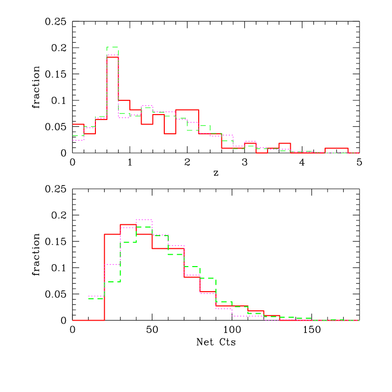
Figure 43: Normalized redshift distribution (upper panel) and net detected counts (lower panel) for the subsample of real sources with flat spectrum (continuous lines) and for sources simulated with a pexrav spectral model (dashed lines – Simulation 1) and with a zwabs pow spectral model (dotted lines – Simulation 2).

We also assume for simplicity, that all the sources can be described by two possible spectral shape: an absorbed power law for Compton thin sources, and a pure reflection for Compton thick sources. With the command fakeit within XSPEC, we simulated 1000 sources with a pure cold reflection spectrum, pexrav in XSPEC, with $\Gamma$ fixed to 1.8 and all the other parameters set to the default values (Simulation 1). Each simulated source is assigned a redshift and a normalization according to the distribution of the redshifts and the net detected counts of the subsample of real sources. Then, we simulated another 1000 sources with an absorbed power law (zwabs pow model), with a similar redshift and net detected counts distributions (Simulation 2). In Figure 43 we compare the redshift and net detected counts distributions of the simulated sources with that of the parent sample of real sources. The values of $N_{H}$ for the sources simulated with the model zwabs pow, are consistently extracted from the distribution we found in the paper (but only for $N_{H}<10^{24}$ cm^-2 to exclude Compton thick sources).

Then, we analyzed the two sets of simulation both with the pexrav (appropriate only for Simulation 1) and zwabs pow (appropriate only for Simulation 2) model. We verified that in the the first case we succesfully recover the input values for the normalization of the pexrav spectra, and in the second case the input values for $N_{H}$, within the errors. Finally, we compute the difference between the Cash-statistics obtained with the zwabs pow model and that obtained with the pexrav model: $\Delta C=C_{zwapow}-C_{pexrav}$. The normalized distributions of the values of $\Delta C$ are shown in Figure 44. We recall that we have two free parameters for the zwabs pow model and only one for the pexrav model; this explains why the distribution of Simulation 2 has a much larger tail at negative values of $\Delta C$. Our goal is to use these distributions to choose a fixed threshold $\tilde{\Delta}C$ that allows us to select Compton thick candidates among the parent sample. The optimal choice would minimize the number of Compton thin sources mistakenly included in the C–thick sample, at the same time recovering the largest fraction of the Compton thick population.

The distribution of $\Delta C$ for Simulation 1 is skewed towards large positive values, as expected since the pexrav model is the correct one. The tail at low values of $\Delta C$ is a measure of how many Compton thick sources may be missed when choosing a fixed threshold in $\Delta C$. The distribution of $\Delta C$ for Simulation 2 is centered around negative values, since here the pexrav model is not appropriate. Therefore, the tail at high values of $\Delta C$ is a measure of how many sources with an actual zwabs pow spectrum are mistakenly selected as C–thick candidates for a fixed threshold in $\Delta C$.

The simplifying assumption that our subsample of real sources includes only C–thin and C–thick sources, reads $N_{tot}=N_{C-thick}+N_{C-thin}$ where $N_{tot}$ is the total number of sources in the subsample (here 110). We collect $N_{C}$ sources as C–thick candidates by selecting the sources from the parent sample for which $\Delta C>\tilde{\Delta}C$. The expected value for $N_{C}$ is:

$$N_{C}=N_{C-thick}\,*\,F1+N_{C-thin}\,*\,F2\,,$$ (4)

where $F_{1}$ and $F_{2}$ are the probabilities that a C–thick source is correctly recovered, and that a C–thin source is mistakenly included among the C–thick candidates, respectively. We can estimate $F_{1}$ and $F_{2}$ by integrating the two distributions for $\Delta C>\tilde{\Delta}C$.

Therefore, the actual fraction of the C–thick sources in the parent sample $f_{CT}\equiv N_{C-thick}/N_{tot}$ can be estimated as:

$$f_{CT}=\Large(N_{C}/N_{tot}-F_{2}\Large)/(F_{1}-F_{2}).$$ (5)

Our estimated $f_{CT}$ should not depend on $\tilde{\Delta}C$ if our initial assumption $N_{tot}=N_{C-thick}+N_{C-thin}$ is correct. However, we know that the picture may be complicated by the presence of sources with soft component, or the lack of a proper treatment of the Compton scattering when $N_{H}$ approach the Compton thick value of $1.5\times 10^{24}$ cm^-2 (which would require the use of the model plcabs). However, a more detailed treatmend would go beyond the scope of this Paper. We find that for $\Delta C>1$ the expected values for $f_{CT}$ ranges between 0.10 and 0.20 (see Figure 45). Note here that this fraction is computed among the parent sample of 110 sources, therefore it corresponds to a number between only 10 and 20 C–thick sources in the whole CDFS sample.

Obviously, for higher values of $\Delta C$, the quality of the C–cthick condidates sample is increasing, while the fraction of true C–thick sources actually recovered drops. Assuming $f_{CT}\simeq 0.15$, we plot in figure 46 the following quantities as a function of $\Delta C$: the expected fraction of true C–thick sources among the candidates ($f_{good}$); the expected fraction of spurious sources among the candidates ($f_{sp}$); the fraction of the total C–thick source population actually recovered ($f_{rec}$). We notice that for $\Delta C\leq 2$ more than 50% of the total C–thick source population is recovered. Therefore we assume $\tilde{\Delta}C=2$.

The number of C–thick candidates we find for $\tilde{\Delta}C=2$ is 14 (see text). The number of spurious sources among the C–thick candidates turns out to be still significant, between 3 and 5. To summarize, we demonstrated here that a selection of C–thick sources on the basis of the X–ray spectrum is feasible. We also show that we can quantify the completeness and the contamination of our C–thick candidate sample. We also notice that the level of contamination is not negligible, pointing towards the need of a more sophisticated X–ray spectral analysis, including, for example, the systematic search for the Fe line expected more frequently in reflection–dominated spectra, or considering the presence of a soft component that can mimick a flat spectrum (see Weaver et al. 1996). Overall, we believe that a refined version of this approach can constitute a valuable tool to look for Compton thick sources on the basis of the X–ray data only.

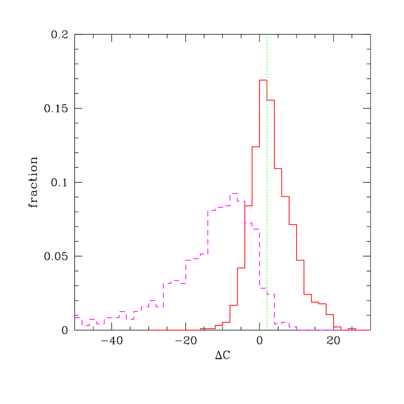
Figure 44: Normalized distribution of $\Delta C$ for Simulation 1 (continuous line) and for Simulation 2 (dashed line). The vertical dotted line correspond to the choosen threshold $\Delta C=2$.

Figure 45: Estimated value of the fraction of C–thick sources among the parent sample (110 sources) as a function of $\Delta C$ according to eq. 5.

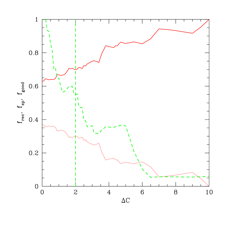
Figure 46: Upper solid line: expected fraction of true C–thick sources among the candidates ($f_{good}$) versus $\Delta C$; lower solid line: expected fraction of spurious sources among the candidates ($f_{sp}$); dashed line: fraction of the total C–thick source population actually recovered ($f_{rec}$).

Appendix C Measures of $N_{H}$ at high–z: simulations

The best fit values of $N_{H}$ may show a spurious trend with redshift, due to the increasing difficulty of measuring $N_{H}$ when the rest–frame soft band, which is most sensible to the intrinsic absorption, is shifted out of the Chandra energy range. What happens typically is that the error bars are so large that, while the upper limits to $N_{H}$ increase with redshift, the best fit values may fluctuate at large positive values also when the source has a negligible intrinsic absorption. We take into account part of this effect by resampling the value of $N_{H}$ according to the error bars, however since $N_{H}$ is always defined as positive, it is hard to avoid an average trend of increasing intrinsic absorption with redshift. In particular, we asked ourselves if the absorbed BLAGN found at $z>2$ may be spurious (see §7).

To investigate this effect, we performed three sets of simulations (100 spectra each) of sources with negligible absorption (equal to the galactic value $9\times 10^{19}$ cm^-2) with redshift distributed uniformly in the range $z=0-4$. The average number of net detected counts in each set of simulations is 490, 150 and 80. In Figure 47 we show the best fit values of $N_{H}$ (with 1 $\sigma$ error bars) plotted versus redshift. We also plot separately the cases in which $N_{H}>0$ at more than 1 $\sigma$. We notice that, while the upper limits increases following approximately the $(1+z)^{3}$ law, the number of false detections of a non–negligible intrinsic absorption ($N_{H}>0$ at more than 1 $\sigma$) is not increasing significantly with redshift. In addition, we find that at 2 $\sigma$ confidence level, all the values of $N_{H}$ are consistent with negligible absorption.

Therefore, the sample of BLAGN we discuss is consistent with no absorption in average (since $N_{H}=0$ for all the BLAGN at 2 $\sigma$ c.l.). However the number of sources with best fit value $N_{H}>10^{22}$ cm^-2 among the BLAGN is 7, and it is larger than that expected for negligible absorption on the basis of the simulations (which is about 3). We conclude that some of the high–z BLAGN do have absorption at the level of $N_{H}\sim 10^{21}$ cm^-2, still consistent with that found in Type I AGN. Values typical of Type II AGN, larger than $10^{22}$ cm^-2, would have been detected, while values around $10^{21}$ cm^-2 are compatible with what we found in the data (see Figure 48). This picture is confirmed by the analysis of the XMM data for these sources (see discussion in §7).

To summarize, we find that the effect of an artificially increasing measure of intrinsic absorption with redshift is under control in our sample. A complete removal of the spurious trend would need extensive simulations and several iterations, since the effect depends on the actual behaviour of $N_{H}$ with redshift. Such an approach goes beyond the scope of this Paper, but it should be adopted for larger AGN samples.

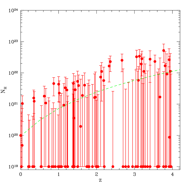
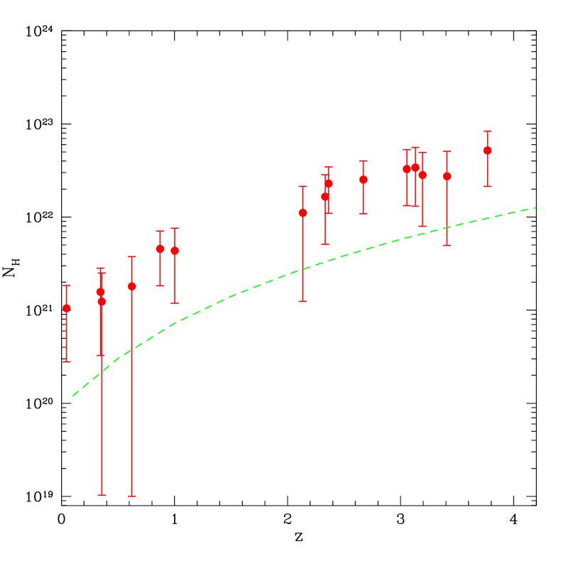
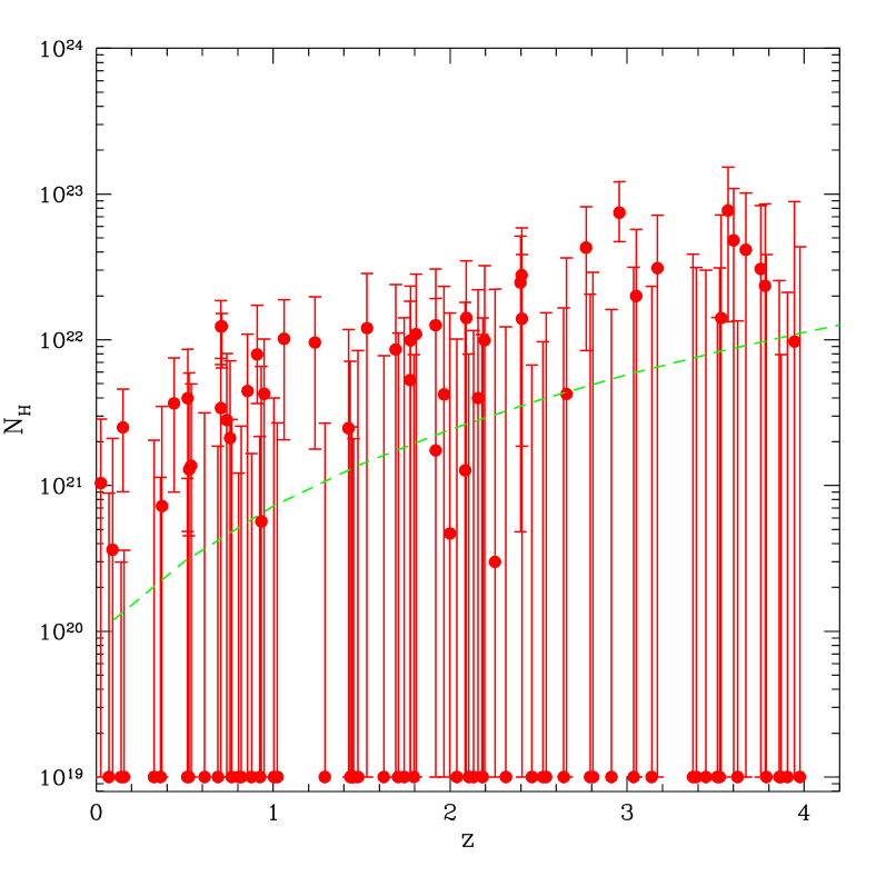
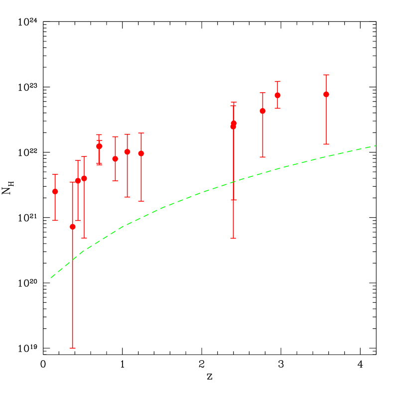
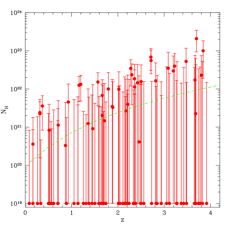
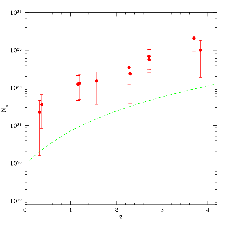
Figure 47: Lef panels: Best fit values of $N_{H}$ as a function of redshift for simulated sources with input values $N_{H}=9\times 10^{19}$ cm^-2. The dashed line is $9\times 10^{19}(1+z)^{3}$. Error bars correspond to 1 $\sigma$. The typical net detected counts are 480, 150 and 80 from top to bottom. Right panels: values of $N_{H}$ for which $N_{H}>0$ at 1 $\sigma$.

Figure 48: Best fit values of $N_{H}$ as a function of redshift for simulated sources with input values $N_{H}=5\times 10^{22}$ cm^-2 (left panel) and $N_{H}=10^{21}$ cm^-2 (right panel). Error bars correspond to 1 $\sigma$. The typical net detected counts are 280 (left panel) and 470 (right panel).