Zeeman tomography of magnetic white dwarfs

Abstract

Aims. We analyse the magnetic field geometry of the magnetic DA white dwarf PG 1015+014 with our Zeeman tomography method.

Methods. This study is based on rotation-phase resolved optical flux and circular polarization spectra of PG 1015+014 obtained with FORS1 at the ESO VLT. Our tomographic code makes use of an extensive database of pre-computed Zeeman spectra. The general approach has been described in Papers I and II of this series.

Results. The surface field strength distributions for all rotational phases of PG 1015+014 are characterised by a strong peak at 70 MG. A separate peak at 80 MG is seen for about one third of the rotation cycle. Significant contributions to the Zeeman features arise from regions with field strengths between 50 and 90 MG. We obtain equally good simultaneous fits to the observations, collected in five phase bins, for two different field parametrizations: (i) a superposition of individually tilted and off-centred zonal multipole components; and (ii) a truncated multipole expansion up to degree $l=4$ including all zonal and tesseral components. The magnetic fields generated by both parametrizations exhibit a similar global structure of the absolute surface field values, but differ considerably in the topology of the field lines. An effective photospheric temperature of $T_{\mathrm{eff}}$ = 10 000 $\pm$ 1000 K was found.

Conclusions. Remaining discrepancies between the observations and our best-fit models suggest that additional small-scale structure of the magnetic field exists which our field models are unable to cover due to the restricted number of free parameters.

1 Introduction

In about 170 of the 5448 white dwarfs (WDs) listed in the Web Version of the Villanova White Dwarf Catalog magnetic fields between 2 kG–1000 MG have been detected, corresponding to a fraction of $\simeq$ 3 % (McCook & Sion 1999; Wickramasinghe & Ferrario 2000; Vanlandingham et al. 2005). Most of the WDs have not been scrutinisingly examined for the presence of a magnetic field, however, and a statistical study suggests that the true fractional incidence could be as high as 20 % (Liebert et al. 2003; Schmidt et al. 2003). The magnetic white dwarfs (MWDs) are widely believed to be the successors of the chemically peculiar magnetic Ap stars, which are the only main sequence stars to show substantial globally organised magnetic fields. However, this scenario is challenged by the recent detections of kilogauss-size fields in several MWDs as well as in their direct progeny (central stars of planetary nebulae and hot subdwarfs, Aznar Cuadrado et al., 2004, Jordan et al., 2005, O’Toole et al., 2005). Undoubtedly, further theoretical and observational efforts are required in order to shed more light on the role magnetic fields play in the key stages of post-main sequence evolution. For the present purpose, we consider MWDs as stars displaying a field strength $B\ga 1$ MG.

Due to the intrinsic faintness of WDs, 8-m class telescopes are required in order to record high-quality spectropolarimetric data with sufficient time resolution as a basis for studies of the magnetic field geometry. In the course of our Zeeman tomography programme we have conducted observations for a number of isolated (non-accreting) and accreting MWDs at the ESO VLT with FORS1 in the spectropolarimetric mode.

Figure 1: Left panel: Flux spectra of PG 1015+014 from May 1999. The uppermost 11 spectra have been shifted upwards by 2 flux units, respectively. Right panel: Combined flux and circular polarization spectra of PG 1015+014 from the May 1999 observations. These spectra, which have been collected into five phase bins, will be used as input spectra for the Zeeman tomography procedure. For clarity, the uppermost four flux spectra have been shifted upwards by 1.5 flux units, respectively. The tick marks below the top axis indicate the wavelengths that were used to adjust the continuum flux level of the the model spectra to the observations.

In the present work – the third paper of our series on Zeeman tomography – we present an application of our code to observations of the non-accreting white dwarf PG 1015+014 and find a field geometry that deviates strongly from centred dipoles or quadrupoles. In the first paper of the series, we have demonstrated that Zeeman tomography is a suitable method to recover field geometries by analysing synthetically generated spectra (Euchner et al. 2002, hereafter Paper I). In a first application of this theory, we have derived a quadrupole-dominated field structure with a prevailing field of $\simeq$ 16 MG for HE 1045$-$0908 (Euchner et al. 2005, hereafter Paper II).

The magnetic DA white dwarf PG 1015+014, discovered in the Palomar Green survey (Green et al. 1987), was observed by Wickramasinghe & Cropper (1988, hereafter WC88) with the RGO spectrograph at the AAT in the wavelength range 4000–7000 Å. Their phase-resolved spectroscopy and low-resolution circular polarimetry revealed significant modulations in flux and circular polarization ($V/I$) over the rotation cycle. From nearly sinusoidal oscillations of the wavelength-averaged degree of circular polarization between $-$1.5 % and 1.5 % the authors derived a rotational period of $P_{\mathrm{rot}}$ = 98.7 min, which was later confirmed with higher accuracy by Schmidt & Norsworthy (1991) who used white-light circular polarimetry. In the individual polarization spectra of WC88, $|V/I|$ is $\simeq$ 5 % in the continuum and up to $\simeq$ 10 % in individual features. They fitted theoretical MWD model spectra to the observations and found an obliquely rotating magnetic dipole model with a polar field strength of $B^{\mathrm{d}}_{\mathrm{pol}}$ = 120 $\pm$ 10 MG and an almost equator-on view to be the best-fitting field geometry. Remaining discrepancies between observations and model spectra were attributed to higher-field regions superimposed on the dipolar field structure. Our analysis provides a substantially improved insight into the field structure of PG 1015+014.

2 Observations

We have obtained spin-phase resolved circular spectropolarimetry of PG 1015+014 with FORS1 at the ESO VLT on May 15, 1999. The spectrograph was operated in spectropolarimetric (PMOS) mode, with the GRIS_300V+10 grism and an order separation filter GG 375, yielding a usable wavelength range $\sim$ 3850–7900 Å. With a slit width of 1″  the FWHM spectral resolution was 13 Å at 5500 Å. The observational data have been reduced according to standard procedures (bias, flat field, night sky subtraction, wavelength calibration, atmospheric extinction, flux calibration) using the context MOS of the ESO MIDAS package. The instrumental setup and the data reduction are analogous to those employed for our analysis of HE 1045$-$0908 (Paper II).

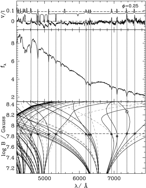
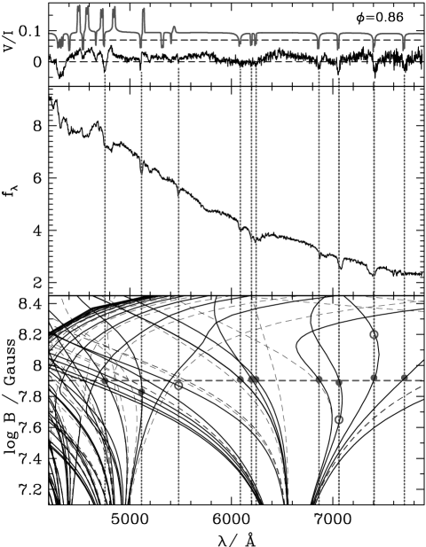
Figure 2: Zeeman maximum ($\phi=0.25$, left panel) and minimum ($\phi=0.86$, right panel) flux ($f_{\lambda}$) and circular polarization ($V/I$) spectra for PG 1015+014, plotted along with the theoretically predicted field-dependent transition wavelengths for Balmer absorption lines ($\lambda$–$B$ curves). Transitions corresponding formally to $|\Delta l|=0,2,4,\dots$ with the zero-field angular momentum quantum number $l$ have been plotted as dashed curves in the bottom parts of the figures. Filled circles denote unambiguous identifications of transitions, open circles less certain ones. In the top parts, theoretical circular polarization spectra are shown for comparison (shifted upwards for clarity, see the text for the adopted model parameters). $f_{\lambda}$ is given in units of $10^{-16}$ erg cm^-2 s^-1 $\AA^{-1}$.

We secured a sequence of 12 exposures with an exposure time of 8 min each, covering a full rotation cycle. We were able to reach a signal-to-noise ratio $S/N\simeq 100$ for the individual flux spectra (Fig. 1, left panel). The wavelength-dependent degree of circular polarization ($V/I$) was computed from two consecutive exposures – with the retarder plate positions differing by 90° – in order to eliminate Stokes parameter crosstalk, thus yielding six independent phase bins. The flux spectra do not show the typical absorption signature of low- and intermediate-field MWDs with the H$\alpha$ $\pi$ component at the zero-field wavelength surrounded by broader $\sigma^{-}$ and $\sigma^{+}$ troughs, but exhibit a variety of distinct sharp lines scattered over the whole optical range which vary in strength, position, and shape with the rotational phase. The continuum circular polarization differs significantly from zero for most phases. Both phenomena are characteristic of a high-field object with $B\ga 50$ MG (e.g. Wickramasinghe & Ferrario 2000).

We collect the observed flux and circular polarization spectra into five nearly-equidistant phase bins ($\phi=0.05$, 0.25, 0.45, 0.66, 0.86). The phases refer to the ephemeris of Schmidt & Norsworthy (1991) with $\phi=0$ denoting the change from positive to negative continuum polarization. These flux and polarization spectra (Fig. 1, right panel) form the basis of our tomographic analysis. We investigate two particular phases in greater detail: $\phi=0.25$, when the Zeeman features are strongest (“Zeeman maximum”); and $\phi=0.86$, when they are weakest (“Zeeman minimum”).

3 Qualitative analysis of the magnetic field geometry

As a first step of the analysis, we compare the positions and strengths of the most prominent features in the observed spectra with the expected field-dependent wavelengths of the hydrogen transitions $\lambda^{\textrm{H}}(B)$, henceforth referred to as $\lambda$–$B$ curves (Forster et al. 1984; Rösner et al. 1984; Wunner et al. 1985). In Fig. 2, we show the observed flux and circular polarization spectra along with the $\lambda$–$B$ curves for $\phi=0.25$ (left panel) and 0.86 (right panel). Transitions that could be unambiguously identified with specific spectral features have been marked with filled grey circles and are listed in Table 1. Possible or unlikely identifications are displayed as open circles. In the presence of an electric field additional transitions can occur which formally correspond to $|\Delta l|=0,2,4,\dots$, with $l$ being the angular momentum quantum number in the zero-field nomenclature. These components have been plotted as dashed curves in the bottom parts of Fig. 2.

Table 1: Positions of observed Zeeman features and corresponding Balmer transitions. A colon denotes a less certain identification.

$\lambda$ / Å	Transition	$\lambda$ / Å	Transition
($\phi=0.25$)		($\phi=0.86$)
4610	H$\beta$ (2s 0 $\rightarrow$ 4f 0)	4755	H$\beta$ (2p 0 $\rightarrow$ 4d$-$1)
	H$\beta$ (2p+1 $\rightarrow$ 4s 0)	5115	H$\beta$ (2s 0 $\rightarrow$ 4f$-$1)
4805	H$\beta$ (2p 0 $\rightarrow$ 4d$-$1)	5480	H$\alpha$ (2p 0 $\rightarrow$ 3s 0) :
5117	H$\beta$ (2s 0 $\rightarrow$ 4f$-$1)	6088	H$\alpha$ (2p$\pm$1 $\rightarrow$ 3d$\pm$1)
5326	H$\alpha$ (2p$-$1 $\rightarrow$ 3d 0)	6198	H$\alpha$ (2s 0 $\rightarrow$ 3p 0)
	H$\beta$ (2p+1 $\rightarrow$ 4d 0)	6243	H$\alpha$ (2p 0 $\rightarrow$ 3d 0)
5475	H$\alpha$ (2p 0 $\rightarrow$ 3s 0) :	6864	H$\alpha$ (2p+1 $\rightarrow$ 3s 0)
6193	H$\alpha$ (2p$\pm$1 $\rightarrow$ 3d$\pm$1)	7060	H$\alpha$ (2s 0 $\rightarrow$ 3p$-$1)
6268	H$\alpha$ (2s 0 $\rightarrow$ 3p 0)	7405	H$\alpha$ (2p$-$1 $\rightarrow$ 3d$-$2)
6326	H$\alpha$ (2p 0 $\rightarrow$ 3d 0)	7705	H$\alpha$ (2p 0 $\rightarrow$ 3d$-$1)
6927	H$\alpha$ (2p+1 $\rightarrow$ 3s 0)
7085	H$\alpha$ (2s 0 $\rightarrow$ 3p$-$1)
7369	H$\alpha$ (2p$-$1 $\rightarrow$ 3d$-$2)
7594	H$\alpha$ (2p 0 $\rightarrow$ 3d$-$1)

In the Zeeman maximum spectrum ($\phi=0.25$), three H$\alpha$ $\pi$ and four H$\alpha$ $\sigma^{+}$ transitions with $\lambda>6000$ Å are clearly visible as positive peaks superimposed on a negative polarization continuum. In particular, the narrow feature at 7085 Å which corresponds to a local extremum of the 2s 0 $\rightarrow$ 3p$-$1 $\lambda$–$B$ curve allows a reliable estimation of the prevailing field strength. For $\lambda<6000$ Å, we identify three strong features showing positive polarization (at 4610, 4805, and 5117 Å) with H$\beta$ $\sigma^{+}$ transitions. Our identifications of several line features differ from those suggested by WC88 for the same rotational phase. The feature at 5326 Å shows a noticeable negative polarization and is interpreted as a blend of a H$\alpha$ $\sigma^{-}$ and a H$\beta$ $\sigma^{+}$ component, with the 2p$-$1 $\rightarrow$ 3d 0 transition dominating. The strong line at 5475 Å with positive polarization probably arises from the H$\alpha$ $\pi$ transition 2p 0 $\rightarrow$ 3s 0. The feature at 5930 Å reported by WC88 is not present in our data. Furthermore, there is a distinct feature with a positive peak in polarization at 5200 Å which they attribute to the H$\alpha$ $\sigma^{-}$ transition 2p+1 $\rightarrow$ 3d+2. We question this identification because the H$\alpha$ $\sigma^{-}$ components produce lines with strong negative polarization. However, no obvious match with a specific $\lambda$–$B$ curve can be found in Fig. 2, so the origin of this feature remains unclear. We do not attempt to identify spectral features at wavelengths $\lambda<4600$ Å because the number of candidate transitions from the overlapping H$\beta$ and H$\gamma$ manifolds is too large. Taking into account all these identifications, we conclude that the distribution of the corresponding field strengths must be centred quite sharply at $\simeq$ 70 MG. To illustrate this, we show in the top part of Fig. 2 (left panel) a theoretical circular polarization spectrum for a single value $B=69$ MG with $\psi=51$°, and $T_{\mathrm{eff}}=10$ 000 K, where $\psi$ denotes the viewing angle between the magnetic field direction and the line of sight.

In the Zeeman minimum spectrum ($\phi=0.86$), the absorption signature for $\lambda>6000$ Å is similar to that at Zeeman maximum, although the H$\alpha$ $\pi$ line components are not visible as separate peaks in $V/I$, but rather produce a broad depression of the overall positive continuum polarization. The H$\alpha$ $\sigma^{+}$ components are wider than those at $\phi=0.25$. Both effects suggest a broader distribution of field strengths at Zeeman minimum. A theoretical circular polarization spectrum for a single value $B=82$ MG, $\psi=129$°, and $T_{\mathrm{eff}}=10$ 000 K provides a good indication for the prevailing field strength and direction. As can be seen from the change of polarity in the continuum circular polarization, the net magnetic field direction has changed sign along the line of sight. The fact that for both phases, which are separated by about half a rotation cycle ($\Delta\phi=0.39$), the field distributions seem to be clearly peaked at values differing by only $\simeq$ 20 % indicates a field geometry more complex than centred or off-centred dipoles or quadrupoles.

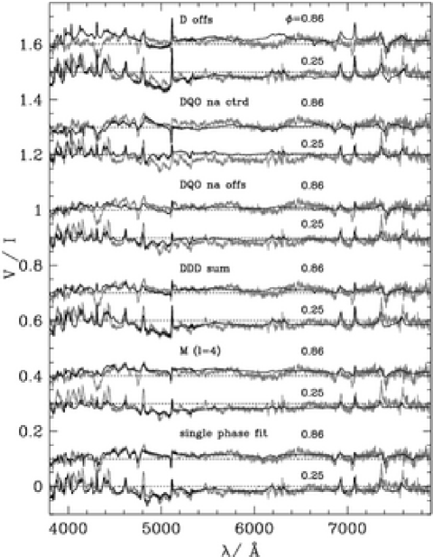
Figure 3: Observed circular polarization spectra for phases $\phi=0.25$ and 0.86 (grey curves) and best-fit synthetic spectra (black curves) for different parametrizations of the magnetic field geometry. From top to bottom: off-centred dipole (D offs); centred, non-aligned combination of dipole, quadrupole, and octupole (DQO na ctrd); off-centred, non-aligned combination of dipole, quadrupole, and octupole (DQO na offs); superposition of three individually off-centred, non-aligned dipoles (DDD sum); truncated multipole expansion up to degree $l=4$. The lowermost two curves show individual fits to single phases with a truncated multipole expansion up to $l=5$ ($\phi=0.25$) and $l=4$ ($\phi=0.86$). All curves except for the bottom one have been shifted vertically by suitable amounts in $V/I$, with the horizontal dashed lines indicating the respective levels of zero polarization.

Table 2: Best-fit magnetic parameters for the different parametrizations of the magnetic field shown in Fig. 3. The uncertainties in the last digit are denoted by the values in brackets. For each model, a short description is given in the first line. The best-fit inclinations are 24° $\pm$ 3 ° (model 1), 45° $\pm$ 3 ° (model 2), and 36° $\pm$ 4 ° (model 3). The superscripts ‘d’, ‘q’, and ‘o’ refer to dipole, quadrupole, and octupole, the subscript ‘pol’ to the polar field strength. The last three columns give the offsets in units of the white dwarf radius. Formulae for the field structure are given in Paper I.

$B^{\mathrm{d}}_{\mathrm{pol}}$	$\Theta^{\mathrm{d}}$	$\Phi^{\mathrm{d}}$	$B^{\mathrm{q}}_{\mathrm{pol}}$	$\Theta^{\mathrm{q}}$	$\Phi^{\mathrm{q}}$	$B^{\mathrm{o}}_{\mathrm{pol}}$	$\Theta^{\mathrm{o}}$	$\Phi^{\mathrm{o}}$	${x^{\prime}}_{\mathrm{off}}$	${y^{\prime}}_{\mathrm{off}}$	${z^{\prime}}_{\mathrm{off}}$
(MG)	(°)	(°)	(MG)	(°)	(°)	(MG)	(°)	(°)	($R_{\mathrm{WD}}$)	($R_{\mathrm{WD}}$)	($R_{\mathrm{WD}}$)
(1) D offs (off-centred dipole)
$-$97 (2)	85 (3)	77 (4)	–	–	–	–	–	–	$-$0.113 (5)	$-$0.0036 (2)	0.162 (4)
(2) DQO na ctrd (non-aligned, centred combination of dipole, quadrupole, and octupole)
$-$1.4 (1)	53 (13)	325 (6)	13.9 (6)	26 (2)	115 (5)	174 (1)	65 (3)	94 (5)	–	–	–
(3) DQO na offs (non-aligned, off-centred combination of dipole, quadrupole, and octupole)
$-$38 (2)	85 (3)	82 (5)	$-$15 (3)	85 (5)	21 (3)	171 (6)	75 (6)	102 (5)	0.060 (5)	0.011 (1)	0.081 (4)

Table 3: Best-fit magnetic parameters for a superposition of three individually off-centred, non-aligned dipoles (labelled DDD sum in Fig. 3). The individual dipole components are denoted by D1, D2, and D3. The uncertainties in the last digit are given by the values in brackets. The best-fit inclination is 23° $\pm$ 4 °.

	D1	D2	D3
$B^{\mathrm{d}}_{\mathrm{pol}}$ (MG)	$-$40 (2)	92 (5)	$-$38 (3)
$\Theta^{\mathrm{d}}$ (°)	44 (4)	63 (2)	63 (5)
$\Phi^{\mathrm{d}}$ (°)	339 (2)	276 (6)	134 (3)
${x^{\prime}}_{\mathrm{off}}$ ($R_{\mathrm{WD}}$)	0.04 (1)	$-$0.012 (2)	0.27 (1)
${y^{\prime}}_{\mathrm{off}}$ ($R_{\mathrm{WD}}$)	0.35 (3)	$-$0.136 (8)	0.080 (7)
${z^{\prime}}_{\mathrm{off}}$ ($R_{\mathrm{WD}}$)	0.33 (1)	$-$0.28 (3)	0.21 (2)

4 Zeeman tomography of the magnetic field

Our Zeeman tomography synthesises the observed spectra in a best-fit approach. It makes use of an extensive pre-computed database of theoretical flux and circular polarization spectra of magnetic white dwarf atmospheres, with $B$, $\psi$, $T_{\mathrm{eff}}$, $\log g$, and the direction cosine $\mu=\cos\vartheta$ as free parameters, where $\vartheta$ denotes the angle between the normal to the surface and the line of sight. The three-dimensional grid of 46 800 Stokes $I$ and $V$ profiles covers 400 $B$ values (1–400 MG, in 1 MG steps), nine $\psi$ values (equidistant in $\cos\psi$), and 13 temperatures (8000–50 000 K) for fixed $\log g$ = 8 and $\mu=1$. Limb darkening is accounted for in an approximate way by the linear interpolation law  $I_{\lambda}(\mu)/I_{\lambda,\mu=1}=a+b\mu$  with constant coefficients $a=0.53$ and $b=0.47$. The best fit to the absolute flux distribution of PG 1015+014 was obtained with an effective temperature of $T_{\mathrm{eff}}$ = 10 000 $\pm$ 1000 K. We adopt this value in the subsequent analysis.

Table 4: Best-fit magnetic parameters for a truncated multipole expansion up to degree $l=4$ (labelled M in Fig. 3). The coefficients $g_{l}^{m}$ and $h_{l}^{m}$ are in MG. The best-fit inclination is 47°. The tilt and the azimuth of the multipole axis relative to the rotational axis are 22° and 191°.

$m$		$l=1$	2	3	4
0	$g_{l}^{m}$	3.0	0.6	9.0	2.4
1	$g_{l}^{m}$	$-$12.5	19.0	$-$1.0	4.7
	$h_{l}^{m}$	$-$28.2	7.1	$-$15.6	11.0
2	$g_{l}^{m}$	–	$-$19.6	11.6	$-$10.2
	$h_{l}^{m}$	–	$-$15.6	$-$2.4	6.4
3	$g_{l}^{m}$	–	–	4.1	$-$1.7
	$h_{l}^{m}$	–	–	14.9	$-$6.9
4	$g_{l}^{m}$	–	–	–	$-$4.7
	$h_{l}^{m}$	–	–	–	$-$8.8

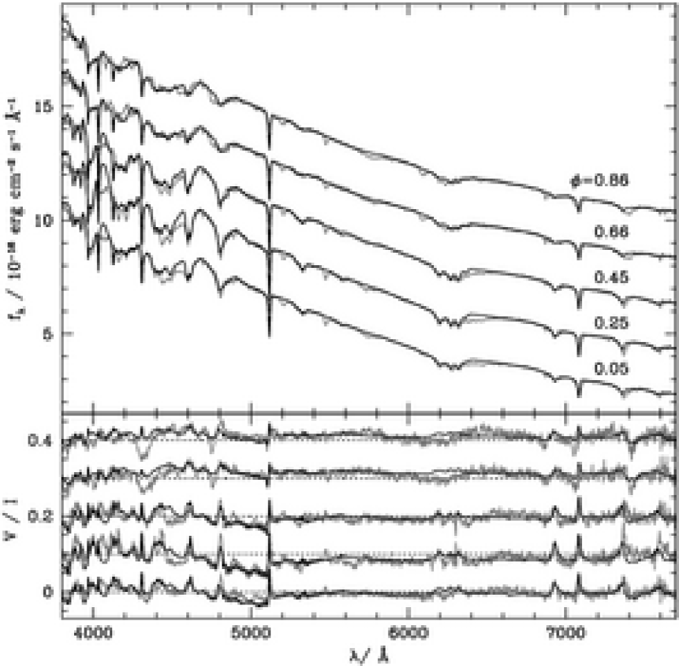
Figure 4: Observed spectra of PG 1015+014 (grey curves) and best-fit synthetic spectra (black curves) using a superposition of three individually off-centred, non-aligned dipoles. The upper four flux (circular polarization) spectra have been shifted for clarity by 2, 4, 6, and 8 (0.1, 0.2, 0.3, and 0.4) units in $f_{\lambda}$ ($V/I$).

In order to determine the misfit between the observations and the model spectra for a given set of magnetic parameters, we use the classical reduced $\chi^{2}$ as our penalty function. The optimisation problem of finding the best-fitting parameters is solved using an evolutionary strategy, implemented by the evoC library (Trint & Utecht 1994). We assign equal statistical weight to the flux and polarization spectra for all five rotational phases and to all wavelengths within the individual spectra. The statistical noise of the observations entering the $\chi^{2}$ function has been estimated by comparing the observed spectra after the application of a Savitzky-Golay filter of 20 Å width with the unprocessed versions. The flux level of the model spectra has been adjusted to the observations at the wavelengths marked with ticks at the top of Fig. 1 (right panel). This is an attempt to remove differences between observed and model flux spectra with wavelengths $\ga 100$ Å, as expected from the remaining uncertainties in the detector response function. We do not correct either for differences between the spectra on shorter wavelengths, nor do we apply any correction to the polarization spectra. The resulting $\chi^{2}_{\mathrm{red}}$ values are of the order of 80 indicating a gross underestimation of the errors which enter the $\chi^{2}$ computation. Larger observational errors and remaining systematic uncertainties in the model spectra probably both contribute to this result. We have experimented with different statistical weights assigned to different wavelength regions – as specific line features or subsections of the continuum – but found no convincing way to better define the goodness of fit. We compromise on using the formal $\chi^{2}_{\mathrm{red}}$, even if large, as a guide line and decide by an admittedly subjective ‘by eye’ process which individual of similarly good fits to accept.

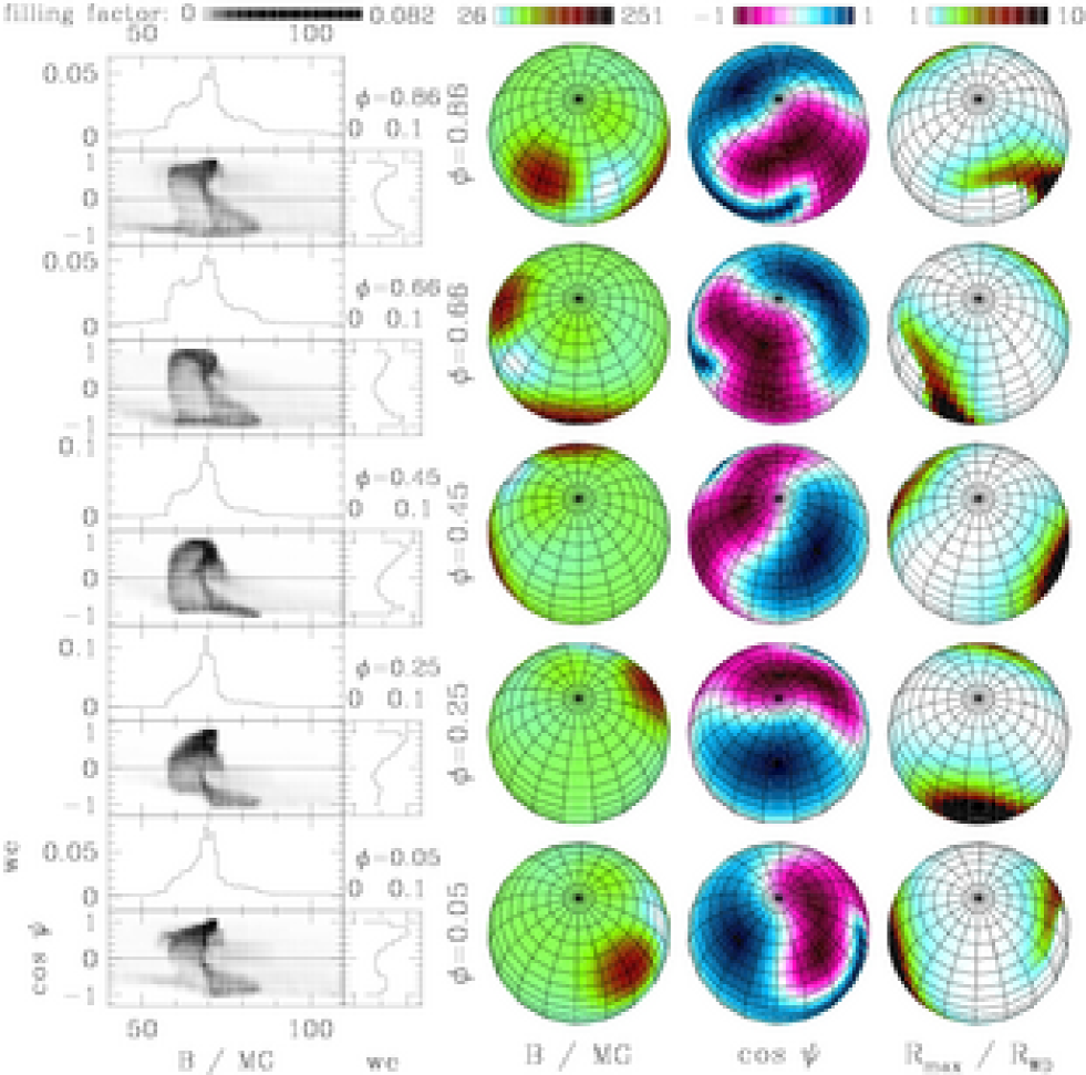
Figure 5: Zeeman tomographic analysis of the magnetic field configuration of PG 1015+014 using a superposition of three individually off-centred, non-aligned dipoles. Left panel: $B$–$\psi$ diagram, right panel: absolute value of the surface magnetic field, cosine of the angle $\psi$ between the magnetic field direction and the line of sight, and maximum radial distance reached by field lines in units of the white dwarf radius.

4.1 Field parametrization

We have embarked on two different strategies in order to find an adequate parametrization of the magnetic field geometry (see also Paper I). The classical approach is that of an expansion of the scalar magnetic potential into a series of spherical harmonics, characterised by degree $l$ and order $m$ with $m=0$ to $l$ for each $l$. Given $l$ and $m$, two free parameters $g_{l}^{m}$ and $h_{l}^{m}$ have to be specified, or one parameter $g_{l}^{0}$ only for the zonal components with $m=0$ (Langel 1987). The approach is powerful, but is limited to the description of rather simple structures if one truncates the expansion at low values of $l$. Such a truncation is necessary in order to avoid convergence problems of the fit, given the rapid growth in the number of fit parameters which increases as $l(l+2)$ for the full $l,m$-expansion. Conceptually simple structures, such as the sum of a quadrupole and octupole with their axes inclined relative to each other, cannot be realised if the series is truncated at low $l\geq 3$. As an alternative approach, we adopt a hybrid model consisting only of zonal ($m=0$) harmonics with independent tilt angles and off-centre shifts. All tesseral components ($m\neq 0$) are ignored in this case. Examples are, e.g., a combination of dipole, quadrupole and octupole, and also a combination of three dipoles independently inclined and offset from the centre. Further details on the field parametrizations are given in Papers I and II.

In the following Section, we proceed systematically from simple structures, as centred or off-centred single zonal components, over the sum of such components, individually tilted and/or offset, to a full multipole expansion truncated at $l=4$. The number of free parameters varies between 4 and 27. In the case of the hybrid model, the fit parameters for each component are the polar field strength $B_{\mathrm{pol}}$, the tilt $\Theta$ and azimuth $\Phi$ of the magnetic axis, and, if applicable, the offsets ${x^{\prime}}_{\mathrm{off}}$, ${y^{\prime}}_{\mathrm{off}}$, and ${z^{\prime}}_{\mathrm{off}}$ from the centre plus the inclination of the rotational axis relative to the line of sight. For the truncated multipole model, we fit the $l(l+2)$ parameters of the model, the two angles of the reference axis, and the inclination.

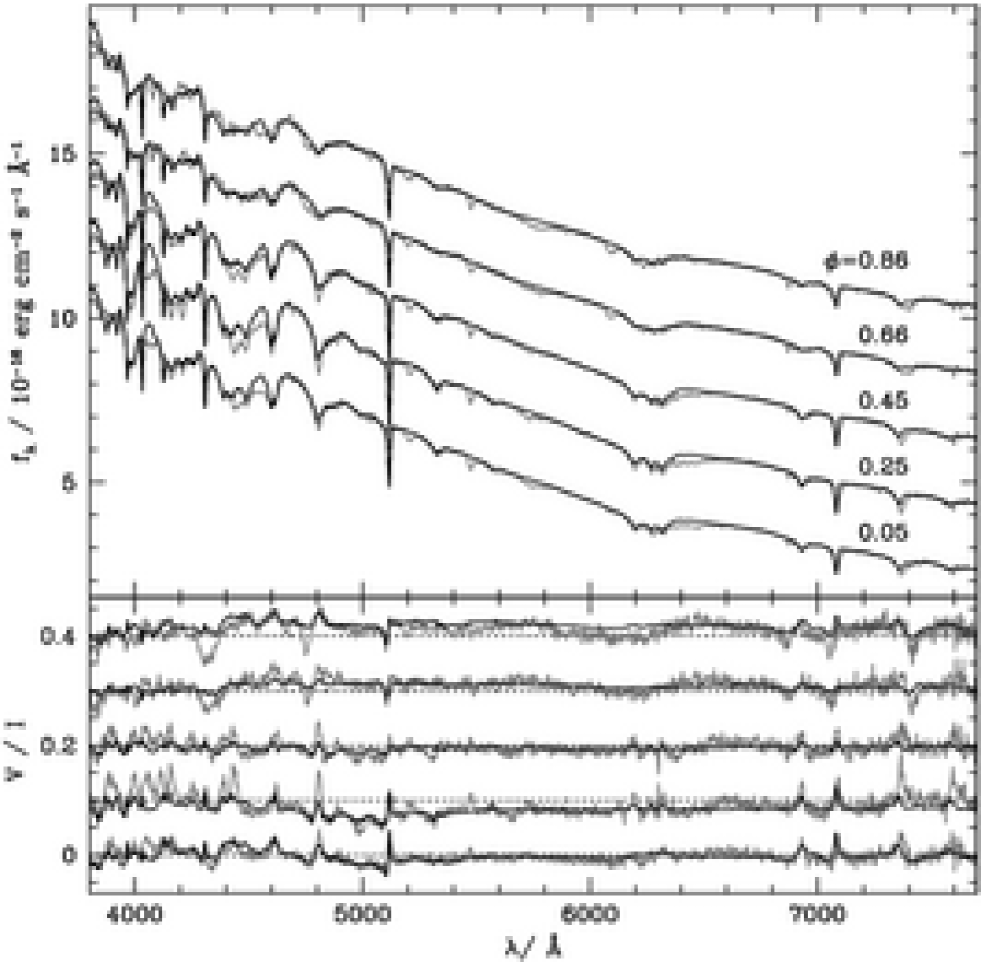
Figure 6: Observed spectra of PG 1015+014 (grey curves) and best-fit synthetic spectra (black curves) for a truncated multipole expansion up to degree $l=4$. For clarity, the upper four flux (polarization) spectra have been shifted upwards by 2, 4, 6, and 8 (0.1, 0.2, 0.3, and 0.4) units in $f_{\lambda}$ ($V/I$).

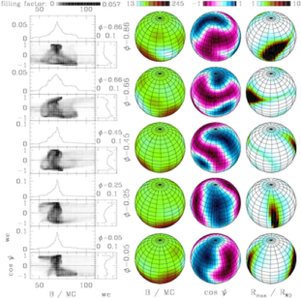
Figure 7: Zeeman tomographic analysis of the magnetic field configuration of PG 1015+014 using a truncated multipole expansion up to degree $l=4$. Left panel: $B$–$\psi$ diagram, right panel: absolute value of the surface magnetic field, cosine of the angle $\psi$ between the magnetic field direction and the line of sight, and maximum radial distance reached by field lines in units of the white dwarf radius.

4.2 Results

For single centred dipoles, quadrupoles, or octupoles no satisfactory fits could be obtained. Nevertheless, we note that the best fit with a centred dipole to the single phase $\phi=0.25$ yielded a value of $B^{\mathrm{d}}_{\mathrm{pol}}$ = 131 $\pm$ 1 MG and an angle of $\alpha=83$° between the magnetic dipole axis and the line of sight, which is compatible with the values quoted by Wickramasinghe & Cropper (1988). The model is far from optimal, however, in particular for the other phases.

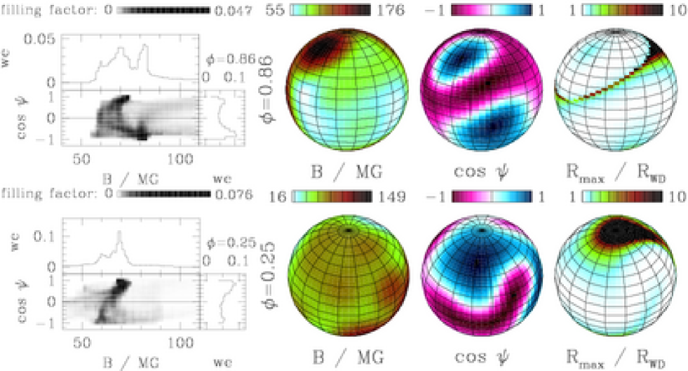
Figure 8: Best-fit results for individual single phase fits to the Zeeman maximum ($\phi=0.25$, bottom panels) and minimum ($\phi=0.86$, top panels) phases. The field has been parametrized by a truncated multipole expansion up to degree $l=5$ for $\phi=0.25$, and up to $l=4$ for $\phi=0.86$. Left panels: $B$–$\psi$ diagram, right panels: absolute value of the surface magnetic field, cosine of the angle $\psi$ between the magnetic field direction and the line of sight, and maximum radial distance reached by field lines in units of the white dwarf radius.

In Fig. 3 we show the observed and best-fitting model circular polarizations at $\phi=0.25$ and 0.86 for selected hybrid and multipole parametrizations with increasing complexity. The simplest configuration is that of an offset dipole (denoted by D offs in Fig. 3). The corresponding values of the magnetic parameters are listed in Table 2. The overall shape of the continuum polarization is reproduced fairly well for all phases, but the model fails seriously in the spectral lines, especially for $\phi=0.86$. For an offset quadrupole, the result was comparably poor. An offset octupole fared slightly better, but still was considered unsatisfactory. While acceptable fits could be obtained with offset dipoles and quadrupoles for HE 1045$-$0908  (Paper II), the magnetic field geometry of PG 1015+014 seems to be significantly more complex.

As a next step, we proceed to the same hybrid field models that yielded successful fits for HE 1045$-$0908. These are produced by the superposition of dipole, quadrupole, and octupole components and the introduction of a common off-centre shift. For the nonaligned centred dipole–quadrupole–octupole combination (DQO na ctrd in Fig. 3), the polarization spectrum at $\phi=0.86$ is reproduced remarkably well, in particular the broad negative dips in polarization at 4310 and 4740 Å, and the 2s 0 $\rightarrow$ 3p$-$1 transition at 7085 Å. The frequency distribution of magnetic field strengths and directions ($B$–$\psi$ diagram, not shown) is double-peaked at fields of 69 and 81 MG in accordance with the considerations of Sect. 3. The essence, however, is that the reproduction is poor for the other phases, including $\phi=0.25$, although $\phi=0.86$ fits well. Introducing a common offset to the model (DQO na offs in Fig. 3) improves the fit at $\phi=0.25$, but shows significant deviations at $\phi=0.86$. As can be seen from the best-fit magnetic parameters in lines (2) and (3) of Table 2, both the centred and the shifted hybrid model are dominated by the octupole component, again suggesting a rather complex geometry. We conclude that the models considered so far still do not suffice to achieve a fair reproduction at all phases.

In an attempt to improve the fits, we stayed with hybrid models and tried to model a star with several field concentrations by adding three dipoles which are individually tilted and off-centred. The model fares surprisingly well despite the absence of quadrupole and octupole components. We conclude that the ability to place and adjust three spots meets reality rather closely. The fit results for this ‘triple dipole’ model are displayed in Fig. 4, Fig. 5, and Table 3 and are discussed below.

Finally, we considered a truncated multipole expansion up to $l=4$ which includes all orders with indices $m=0$ to $l$. This ‘truncated multipole’ model achieves a $\chi^{2}_{\mathrm{red}}$ value similarly good as the triple dipole model and both provide substantially better fits than the parametrizations discussed above if all rotational phases are considered. In particular, the wavelength-dependent level of the continuum circular polarization is reproduced more accurately. The results for the truncated multipole model are shown in Figs. 6 and 7 and in Table 4.

Although both magnetic field topologies are generated by entirely different parametrizations (Tables 3 and 4), the overall appearance of their $B$–$\psi$ diagrams is similar. For both configurations, the visible part of the surface field is dominated by an extended area with a rather small variation of the field strength that leads to the pronounced peaks at $\simeq$ 70 MG in the $B$–$\psi$ diagrams. The phases $\phi=0.25$ and 0.45 are almost entirely dominated by this region of constant (although not homogenous) field. For the remaining phases, the low- and high-field tails of the field strength distribution become more prominent. In the triple dipole model, the regions with low and high fields become manifest as small spots, one of which reaches up to $\simeq$ 160 MG. A second high-field region appears at the stellar limb for phases $\phi=0.66$ and 0.86. For the truncated multipole model, a similarly prominent high-field spot is not seen, but a low-field spot appears close to the stellar limb for $\phi=0.66$ and 0.86 and finds its counterpart in the hybrid model. The high-field regions are divided into two small spots with field values up to $\simeq$ 90 MG and pronounced negative $\cos\psi$, leading to a distinctive signature in the $B$–$\psi$ diagram, and two narrow areas at the stellar limb with $B$ up to $\simeq$ 150 MG and 245 MG, which belong to high-field spots on the hidden part of the stellar surface. This comparison of the triple dipole model and the truncated multipole model emphasises the fact that the principal information on the field structure is contained in the $B$–$\psi$ diagrams. These diagrams indicate that the distributions of the magnetic field are similar, a conclusion which is impossible to draw from the numerical descriptions in Tables 3 and 4.

For both configurations substantial deviations from the observational data remain, e.g., at the broad dips in $V/I$ at 4310 and 4740 Å for phases $\phi=0.66$ and 0.86 which both models cannot reproduce correctly. While it is quite likely that a larger number of free parameters – and, hence, a still further increased complexity of the field – will improve the fits, our present optimisation procedure cannot handle more free parameters and prevents us to pursue this possibility further. As a consequence, it remains unclear what part of the remaining discrepancies, if any, may be due to systematic errors in the model spectra.

A possible way to answer the last question at least in part is to perform fits to the flux and polarization spectra for a single phase and abandon the requirement that the model should simultaneously fit the other phases. The resulting model may be wrong in a global sense, but will provide a more accurate description of the field distribution over the visible hemisphere at the selected phase. Figure 8 shows the resulting $B$–$\psi$ diagrams at $\phi=0.25$ and $\phi=0.86$ using the truncated multipole model with $l=5$ and $l=4$, respectively. The corresponding polarization spectra are shown at the bottom of Fig. 3. The $B$–$\psi$ diagrams differ, in fact, from the distributions for the same phases obtained from the simultaneous fits to all five phases in Figs. 5 and 7. The most obvious new feature is the appearance of a second field maximum at 82 MG for $\phi=0.86$. At $\phi=0.25$, the distributions of the field strengths look similar, but the $\psi$-distributions and, hence, the field geometries differ (see Figs. 5, 7, and 8). We conclude that a major fraction of the misfits still present in our two best global fits is due to the disability of the models to appropriately account for the complexity of the field. The parameter-free spectral synthesis of Donati et al. (1994) would allow to optimise the fit to a single phase still further and answer the quest for the best possible fit with the present database, at the expense of a global field solution, however (see also Section 5).

We conclude that the field models used by us are barely sufficient to describe a single phase of the observations of PG 1015+014, and are certainly not complex enough to describe the global field configuration by fits to all five phases.

Several potential sources of deviations between observations and synthetic model spectra have been proposed in Paper II and arise both from remaining uncertainties on the observational (flat-fielding, flux calibration) and on the theoretical side. Since PG 1015+014 is dominated by substantially higher magnetic field strengths than HE 1045$-$0908, additional error sources for the theoretical model spectra have to be considered. With growing magnetic field strength, for instance, the influence of electric fields on line positions and strengths becomes increasingly important. For the case of arbitrarily oriented electric and magnetic fields no discrete symmetry is left, leading to slightly different transition wavelengths and oscillator strengths than those computed for the diamagnetic case, and even to the occurrence of additional dipole transitions (Faßbinder & Schweizer 1996; Burleigh et al. 1999). Lines of such type have not been included in the atomic data tables used for the computation of our synthetic model spectra and, consequently, cannot be reproduced by our fits. They are possibly responsible for the sharp line features at 5200 Å and 5475 Å and the washed out feature at 5750 Å, which are not explained by our models (Figs. 4 and 6).

Another theoretical uncertainty arises from the simplified treatment of the field-dependent bound-free and free-free transitions as described in Jordan (1992). For the case of Grw $+70^∘8247$ with $B\simeq 320$ MG, Jordan & Merani (1995) have shown that a more consistent but numerically extremely expensive treatment of the continuum opacities can yield slightly different results for the polarization. We regard the uncertainties arising from both potential error sources as relatively small at fields of $\simeq$ 80 MG, but slight deviations from our synthetic spectra cannot be ruled out.

5 Discussion

In this work, we have analysed high-quality spectropolarimetric data of PG 1015+014 covering a whole rotational period with the Zeeman tomography code described in Papers I and II. We have achieved good fits to the observations, but require a magnetic field geometry that is significantly more complex than the popular assumption of centred or moderately offset dipoles and quadrupoles proposed by several authors in the past (Wickramasinghe & Ferrario 2000, and references therein). In fact, the magnetic field structure of PG 1015+014 is even more complex than that derived for HE 1045$-$0908 (Paper II) and can be successfully modelled by two different parametrizations: On the one hand, we used a hybrid model of off-centred, tilted zonal ($m=0$) components, and on the other hand, a truncated multipole expansion including all $m\neq 0$ components. Hence, our results further confirm the evidence that the magnetic field structures of MWDs are non-trivial and require higher multipole components for an accurate description. We have shown, in particular, that a simple oblique dipole model as devised by Wickramasinghe & Cropper (1988) does not suffice to describe the complex Zeeman absorption features.

Our findings for PG 1015+014 show the difficulties that are inherent to the description of a star’s complex magnetic field geometry with only a few numeric parameters. For this object, an appropriate description requires to quote at least the range of field strengths that contributes effectively to the spectral shape, 50 to 90 MG, and the phase-dependent maxima of the field strength distributions at 69 and 82 MG.

For both parametrization strategies the number of free parameters required for a good fit approaches the maximum number our tomography algorithm can currently handle, and we could reach equivalent quality levels for the best fits. The fits are sufficiently good to be certain that the best-fitting field geometry comes reasonably close to reality, but we could not reach the same high quality of the fits as for HE 1045$-$0908 (Paper II).

We propose two explanations for the remaining differences between the observations and our best-fitting models: (i) systematic uncertainties in the model spectra arising already in the field regime at $B\ga 50$ MG, as discussed at the end of Sect. 4.2; (ii) insufficient spatial resolution of the magnetic field distribution provided by our field geometry models. Given the limited number of free field parameters and the corresponding limitations regarding the attainable level of complexity in the $B$–$\psi$ diagrams, residuals caused by both effects cannot be disentangled. However, the fact that fits for a single phase were clearly superior to the simultaneous fits for all five phases suggests that there is room for improvement on the side of finer-grained field distributions. Hence, it would be necessary to examine the quality of fits to all phases with an increased number of free parameters before a reliable estimation of the effects of systematic errors in the synthetic model spectra becomes possible.

A different method to tackle this problem would be an approach like that of Donati et al. (1994), who optimised directly the frequency distribution of field strengths and directions. Such an approach has the advantage that a formal best fit to the observed spectra is found which shows the smallest residuals of all possible combinations of database spectra, but a few potential traps should be kept in mind: (i) there is no unique relation between the $B$–$\psi$ diagram and the field topology (see Paper I for an example of ambiguous field configurations); (ii) there is no guarantee that the derived $B$–$\psi$ diagram corresponds to a field which fits in a globally consistent picture if all rotational phases are regarded; (iii) and it cannot be guaranteed that a distribution of electric currents exists which produces the derived $B$–$\psi$ diagram. Remaining discrepancies between the observations and integrated synthetic spectra derived with the method of Donati et al. (1994) would be, nevertheless, a good measure for the magnitude of systematic errors in the model spectra.

Somewhat unfortunately, the two objects we have analysed so far with our Zeeman tomography code both have equal $T_{\mathrm{eff}}$ (Paper II and this work). It would be desirable to examine the magnetic field geometries of MWDs for a broader range of effective temperatures in order to search for potential effects of a secular field evolution as a function of cooling age.

The outcome of the first three data releases of the Sloan Digital Sky Survey (SDSS) has nearly tripled the number of known MWDs. The multitude of newly found objects covers a broad range of effective temperatures and surface dipole field strengths (Gänsicke et al. 2002; Schmidt et al. 2003; Vanlandingham et al. 2005). Several new objects with $B>200$ MG have been found, while the majority of objects is found in the low-field regime with $B<20$ MG. The SDSS objects provide a vast hunting ground for further systematic studies of the field geometry of MWDs. The SDSS has also nearly doubled the number of helium-rich MWDs and an interesting option is the extension of our Zeeman tomography technique to the synthesis of their spectra. Calculations of the atomic parameters for He are available now and first applications to helium-rich MWDs are available (Jordan et al. 2001; Wickramasinghe et al. 2002).

Another promising avenue of research is the study of accreting MWDs in close mass-transferring binaries. In the following papers of this series, we will investigate the magnetic field structures of the accreting MWDs in magnetic cataclysmic variables.