The formation of molecular clouds in spiral galaxies

Abstract

We present Smoothed Particle Hydrodynamics (SPH) simulations of molecular cloud formation in spiral galaxies. These simulations model the response of a non-self-gravitating gaseous disk to a galactic potential. The spiral shock induces high densities in the gas, and considerable structure in the spiral arms, which we identify as molecular clouds. We regard the formation of these structures as due to the dynamics of clumpy shocks, which perturb the flow of gas through the spiral arms. In addition, the spiral shocks induce a large velocity dispersion in the spiral arms, comparable with the magnitude of the velocity dispersion observed in molecular clouds. We estimate the formation of molecular hydrogen, by post-processing our results and assuming the gas is isothermal. Provided the gas is cold ($T\leq 100$ K), the gas is compressed sufficiently in the spiral shock for molecular hydrogen formation to occur in the dense spiral arm clumps. These molecular clouds are largely confined to the spiral arms, since most molecular gas is photodissociated to atomic hydrogen upon leaving the arms.

1 Introduction

Molecular clouds are the sites of star formation in spiral galaxies (Reddish, 1975; Shu et al., 1987; Blitz & Williams, 1999). As such, they play an important role in the governing the properties of galaxies and their evolution. The properties of molecular clouds have been extensively studied in terms of their emission, kinematics and internal structures (e.g. Dame et al. 1986; Solomon et al. 1987; Brunt 2003; Wilson et al. 2005). Unfortunately they are still poorly understood in terms of their formation and evolution. For example, it is unclear whether the molecular gas is formed in situ from atomic gas or whether molecular clouds are due to the coagulation of pre-existing molecular gas (Blitz & Rosolowsky, 2004; Pringle et al., 2001). Another important question is whether molecular clouds are long lived or just very inefficient at forming stars (Elmegreen, 2000; Hartmann et al., 2001). Inefficient star formation can be potentially explained if the clouds are not globally self-gravitating (Clark & Bonnell, 2004; Clark et al., 2005). In this case, locally bound regions can explain the star formation while the vast majority of the gas escapes the cloud as it is unbound.

Molecular clouds are found to be primarily located in spiral arms of galaxies with an arm to interarm ratio varying from a few in the inner regions of some galaxies (Vogel et al., 1988; Adler & Westpfahl, 1996; Reuter et al., 1996; Brouillet et al., 1998) to greater than 20 in the outer regions of the Milky Way (Heyer & Terebey, 1998; Digel et al., 1996). Since spiral arms are generally defined by the presence of star formation, this concentration of GMCs (giant molecular clouds) to the spiral arms in the Galaxy is not surprising. The total fraction of gas in molecular form also varies from 2 per cent in M33 (Engargiola et al., 2003) to 75 per cent or more in M51 (Scoville & Young, 1983; Garcia-Burillo et al., 1993). However, the detection of CO may be somewhat underestimated due to the uncertainty in the ratio of CO(1-0) luminosity to H₂ mass (the ’X factor’) (Kaufman et al., 1999). Interestingly, the mass spectra of GMCs in galaxies are very similar with $dN\propto m^{-\gamma}dm$, $\gamma$ in the range of 1.5 to 1.8 (Solomon et al., 1987; Heyer & Terebey, 1998). Typical molecular cloud masses in the Milky Way are 100-1000 M_⊙ (Heyer & Terebey, 1998), though GMCs up to 10⁷ M_⊙ have been observed in the Milky Way (Solomon et al., 1987) and M51 (Rand & Kulkarni, 1990).

There are several possibilities regarding the formation of giant molecular clouds (see Elmegreen 1990 and references therein). Where the content of molecular gas is high, e.g. M51 or the centres of galaxies, GMCs could form through the agglomeration of pre-existing molecular clouds (e.g. Scoville & Hersh 1979; Cowie 1980; Tomisaka 1984; Roberts & Stewart 1987). In this scenario, the ISM may be predominantly molecular, but GMCs are only observed where the gas has coalesced into larger structures heated by star formation. However this is unlikely to occur in the outskirts of galaxies or for example, M33, where little molecular gas is thought to exist aside from GMCs (Engargiola et al., 2003). Then other processes, most commonly gravitational/magnetic instabilities (Elmegreen, 1979, 1982; Balbus & Cowie, 1985; Balbus, 1988; Elmegreen, 1989, 1991, 1994) or compression from shocks (Shu et al., 1972; Aannestad, 1973; Hollenbach & McKee, 1979; Koyama & Inutsuka, 2000; Bergin et al., 2004) must be required to convert atomic to molecular gas. Recently, Blitz & Rosolowsky (2004) note that the fraction of molecular gas may depend on a specific factor, such as the gas pressure, whilst the formation mechanism for GMCs is the same regardless of the molecular gas content.

The concentration of GMCs to spiral arms can be explained in one way by the increased local density (Kennicutt, 1989). Alternatively spiral density waves may take a more important role and lead to the direct triggering of star formation (Roberts, 1969; Bonnell et al., 2006). Several models (Bergin et al., 2004; Hollenbach & McKee, 1979; Koyama & Inutsuka, 2000) propose formation of molecular hydrogen through shock compression of the ISM. Thus shocks from spiral density waves could account for the preference of molecular gas in the spiral arms and the significance of spiral arms as sites of star formation.

The properties of molecular clouds include significant structure on all observed scales and supersonic bulk motions that follow the relation $\sigma_{v}\propto R^{1/2}$ (Myers, 1983; Dame et al., 1986; Brunt, 2003; Elmegreen & Scalo, 2004). These kinematics are generally taken to be turbulence and thought to generate the internal structures. An alternative explanation is that structure in the interstellar medium generates the internal velocity dispersion as it passes through a clumpy spiral shock (Bonnell et al., 2006).

Wada et al. (2002) have investigated self-gravitating galactic disks, suggesting that self-gravity of the disk generates turbulence in the ISM. The effect of spiral shocks on the structure of non self-gravitating disks has also been described (Wada & Koda, 2004; Dobbs & Bonnell, 2006). Recent simulations of gravitational collapse in disk galaxies have investigated the dependence of the star formation rate on the Toomre instability parameter and a Schmidt law dependence on the local surface density (Li et al., 2005a). Molecular gas formation has generally been limited to smaller scale studies, e.g. cloud collapse (Monaghan & Lattanzio, 1991) and colliding or turbulent flows (Koyama & Inutsuka, 2000; Audit & Hennebelle, 2005).

In this paper, we look at the dynamics of a non-self-gravitating galactic disk subject to a spiral density wave. We show the formation of clumpy molecular cloud structures in the spiral arms. From Bergin et al. (2004) we take a simple equation for the conversion of atomic to molecular gas which is applied to our galactic simulations. We identify the location of molecular hydrogen in the galactic disk and show the densities required for molecular gas formation.

2 Calculations

We use the 3D smoothed particle hydrodynamics (SPH) code based on the version by Benz (Benz, 1990). The smoothing length is allowed to vary with space and time, with the constraint that the typical number of neighbours for each particle is kept near $N_{neigh}\thicksim 50$. Artificial viscosity is included with the standard parameters $\alpha=1$ and $\beta=2$ (Monaghan & Lattanzio, 1985; Monaghan, 1992).

2.1 Flow through galactic potential

The galactic potential includes components for the disk, dark matter halo and the spiral density pattern. The spiral potential is provided solely by the stellar background, which contains considerably more mass than present in the gas. Thus we ignore the gravitational feedback from the gas to the stellar disk. However, as the background potential is time dependent, the transfer of angular momentum between the potential and the gas is possible (Section 3.6).

We represent the disk by a logarithmic potential

$$\psi_{disk}(r,z)=\frac{1}{2}v_{o}^{2}\log\bigg{(}r^{2}+R_{c}^{2}+\Big{(}\frac{z}{q}\Big{)}^{2}\bigg{)}$$ (1)

e.g. Binney & Tremaine (1987) that provides a flat rotation curve with $v_{0}=220$ km s^-1. The core halo radius is $R_{c}=1$ kpc and $q=0.7$ is a measure of the disk scale height. A further component is the potential for the outer dark matter halo, solved from the density distribution

$$\rho_{halo}(r)=\frac{\rho_{h}}{1+(r/r_{h})^{2}}$$ (2)

where $\rho_{h}=1.37\times 10^{-2}$ M_⊙ pc^-3 is the halo density and $r_{h}=7.8$ kpc the halo radius (Caldwell & Ostriker, 1981). For the spiral density pattern, we use a potential from Cox & Gómez (2002)

$$\begin{split}\psi_{sp}(r,\theta,t)&=-4\pi GH\rho_{0}\exp(-\frac{r-r_{0}}{R_{s}})\sum_{n=1}^{3}\frac{C_{n}}{K_{n}D_{n}}\cos(n\gamma)\\ \text{where}\quad\gamma&=N\bigg{[}\theta-\Omega_{p}t-\frac{\ln(r/r_{0})}{\tan(\alpha)}\bigg{]},\\ K_{n}&=\frac{nN}{r\sin(\alpha)},\\ D_{n}&=\frac{1+K_{n}H+0.3(K_{n}H)^{2}}{1+0.3K_{n}H},\\ C(1)&=8/3\pi,\quad C(2)=1/2,\quad C(3)=8/15\pi\end{split}$$ (3)

The number of arms is given by N and $r_{0}=8$ kpc, $R_{s}=7$ kpc and $H=0.18$ kpc are radial parameters. The pitch angle is $\alpha$, the amplitude of the perturbation $\rho_{0}$ and the pattern speed $\Omega_{p}$. We take N = 4 for a 4 armed potential, and a pitch angle of $\alpha=15^{o}$, comparable with the Milky Way (Vallée, 2005). The 4 armed potential also allows for more frequent passages of the gas through the spiral arms. The pattern speed, $2\times 10^{-8}$ rad yr^-1 leads to a co-rotation radius of 11 kpc. The amplitude of the potential is $\approx 200$ km² s^-2, with $\rho_{0}=1$ atom cm^-3. This corresponds to a perturbation of 3 per cent to the disk potential, and an increase of 20 km s^-1 as gas falls from the top to the bottom of the potential well. Overall the disk is in equilibrium, as the rotational velocities of gas in the disk balances the centrifugal force from the potential. The disk is in vertical equilibrium supported by an initial velocity dispersion. The resulting scale height of the disk is maintained throughout the simulation.

This paper only considers how hydrodynamic forces and galactic potential influence the flow. In particular we do not include the effect of self -gravity, magnetic fields and feedback from star formation. The processes of heating and cooling of the gas are simplified by taking an isothermal equation of state. This approach is taken as our main objective is to assess the dynamics of spiral shocks rather than comprehensively model the ISM.

2.2 Initial conditions

We initially place gas particles within a region of radius 5 kpc$<r<$10 kpc. The disk also has a scale height $z\approx 100$ pc. We allocate positions and velocities determined from a 2D test particle run. The particles in the test particle run are initially distributed uniformly with circular velocities. They evolve for a couple of orbits subject to the galactic potential, to give a spiral density pattern with particles settled into their perturbed orbits.

In the SPH initial conditions, we give the particles velocities in the $z$ direction from a random Gaussian distribution of 2.5% of the orbital speed. We add the same magnitude velocity dispersion in the plane of the disk. The total mass of the disk is nominally $5\times 10^{8}$ M_⊙, but as self-gravity is not included, the total gas mass can be scaled to higher or lower masses. The gas is distributed uniformly on large scales with an average surface density of $\Sigma\approx 2$ M_⊙ pc^-2 and average density of $10^{-2}$ M_⊙ pc^-3. For the higher resolution run, most gas in the interarm regions has densities ranging from $10^{-3}$ M_⊙ pc^-3 to $10^{-2}$ M_⊙ pc^-3 whilst the initial peak density in a spiral arm is $\approx 0.5$ M_⊙ pc^-3 (Figure 1). The nominal surface density ($\approx 2$ M_⊙ pc^-2) is lower than the gas surface density of 5 M_⊙ pc^-2 suggested by (Wolfire et al., 2003) for a radius of 8.5 kpc, although we mainly focus on modelling just the cold phase of the atomic gas. In Section 3.4 we consider the formation of molecular gas with different disk masses and therefore surface densities.

The number of particles is either $10^{6}$ or $4\times 10^{6}$. The higher resolution work was carried out on UKAFF (UK Astrophysical Fluids Facility) whilst the $10^{6}$ particle simulations were run on local computing facilities. We ran simulations for between 200 and 300 Myr, where the orbital periods at 5 and 10 kpc are 150 Myr and 300 Myr respectively. The gas passes through multiple spiral shocks in this time and reaches a steady state. No boundary conditions are applied to our calculations. With $4\times 10^{6}$ particles, the disk is fairly well resolved in the spiral arms, where the ratio of the smoothing length ($h$) to the disk scale height ($H$) is approximately 0.4 (the disk scale height calculated as the height of the disk which contains 2/3 of the local disk mass). However the ratio $h/H$ increases up to $\approx 1$ in the interarm regions.

All calculations are isothermal with temperatures of 10, 50, $10^{2}$, $10^{3}$, or $10^{4}$ K. Most previous simulations and analysis of spiral galaxies (e.g. Wada & Koda 2004; Kim & Ostriker 2002; Dwarkadas & Balbus 1996) assume a sound speed of approximately 10 km s^-1 corresponding to the hotter ($10^{4}$ K) component of the ISM. However, for GMCs to form, gas entering the spiral arms must be cold atomic clouds (Elmegreen, 2002) or pre-existing molecular gas (Pringle et al., 2001). Since our aim of this work is to investigate molecular cloud formation in shocks, lower ISM temperatures are adopted for most of these calculations. We do not include self gravity, but estimate the Toomre parameter for the disk to be $Q\thicksim 2.7$, and so the disk is stable against gravitational collapse. In any case, the gas will reach a spiral arm before gravitational collapse can occur e.g. (Bonnell et al., 2006). We refer to Li et al. (2005b) for a discussion of the stability of disks for different $Q$.

3 Disc dynamics and cloud formation

Figure 1: The distribution of mass as a function of gas density at the beginning (diamonds), after 100 Myr (crosses) and at the end (280 Myr) (squares) of the 50 K simulation. The nominal density for molecular clouds is 2.5 M_⊙ pc^-3.

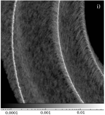
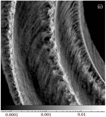
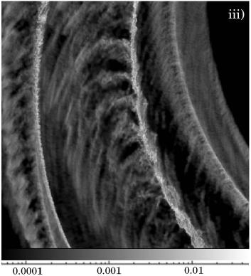
Figure 2: Column density plots (g cm^-2) showing a 5 kpc by 5 kpc section of the disk (with Cartesian coordinates -9 kpc $<x<$ -4 kpc and -5 kpc $<y<$ 0 kpc. The xy-coordinate grid is centred on the midpoint of the disk and remains fixed with time. Gas is flowing clockwise across the disk, i.e. from bottom to top. The time corresponding to each plot is i) 50 Myr, ii) 100 Myr and iii) 150 Myr. This simulation used 4 million particles with a temperature of 50 K.

We first describe briefly the overall structure for the different simulations performed. Section 3.1 then examines the formation of structure in the spiral arms, before we discuss the velocity dispersion across the disk and the distribution of molecular gas.

Initially, the disk is approximately uniform with a smooth spiral perturbation. The widths of the spiral arms are even along the length of each arm, and the densities across the arms are fairly uniform. As the shock develops, the density increases in the spiral arms. In the simulations with cold gas, substructure develops along the spiral arms (Figure 2). The gas in the arms becomes clumpy, and the arm width fluctuates. Densities of gas in the arms varies over approximately two orders of magnitude. The spiral arms become more ragged, and their width increases. Meanwhile dense clumps leaving the arms are sheared, leading to the formation of spurs perpendicular to the arms (Dobbs & Bonnell, 2006). The distribution of gas densities reaches an approximate equilibrium after $\approx 100$ Myr (Figure 1) with gas densities in the spiral arms reaching $>10$ M_⊙ pc^-3. In contrast, the higher temperature simulations show broader, less dense spiral arms (see Dobbs & Bonnell (2006)). The spiral shocks are much weaker for the higher temperature gas, since the change in velocity induced by the spiral potential is more comparable with the sound speed of the gas. For the $10^{4}$ K case, the sound speed is $\approx 10$ kms^-1 whilst the change in velocity across the spiral potential is $\approx 20$ kms^-1 (Section 2.1). The 1000 K simulation shows regular spaced more diffuse clumps along the spiral arms, but the $10^{4}$ K run is relatively featureless, with no obvious structure in the spiral arms. The difference in structure is due to the different strength of the shock and the spacing of the clumps is determined by the spiral arm dynamics (Section 3.1 and Dobbs & Bonnell (2006)).

3.1 Structure formation in the spiral arms

We associate the densest regions of our simulation (Figure 2) with molecular clouds, as they attain the required densities and, as we shall see in Section 4, have appropriate physical conditions and lifetimes that they should be primarily molecular gas. The formation of dense molecular cloud structures can be understood as being caused by the dynamics as interstellar gas passes through a spiral shock. Initially, the pre-shock gas contains small-scale structure due to the particle nature of SPH. The spiral shocks amplify any pre-existing structures such that the clumpiness of the gas increases with each passage through a spiral arm. This amplification of clumpiness corresponds to changes in the angular momentum phase space density of the gas. The pre-shock phase space density is relatively smooth whilst the shocked gas displays much more structure (Figure 3). We provide an explanation of the generation of clumpy structure in terms of this change in the angular momentum of the gas each time it passes through a spiral shock.

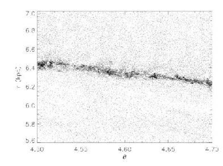
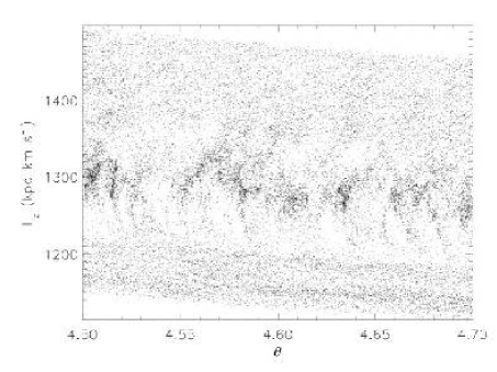
Figure 3: The top figure shows particles in a section of the disk in coordinates ($r,\theta$). $\theta$ is measured in radians clockwise round the disk, and thus the section is taken from the top of the disk. The bottom figure shows the corresponding $z$ component of the angular momentum plotted against $\theta$. The evolution of the structure in the angular momentum phase space is evident in the bottom plot. The clumpy region shows the particles in the spiral shock. Gas below this has yet to pass through the shock and has a relatively smooth distribution. The post-shock gas lies above the clumpy region. The simulation has evolved for 50 Myr.

As the arms are regions of strongly enhanced density, it is evident that gas from a range of radii must interact and shock at any particular point in a spiral arm. These shocks disturb the initially smooth phase-space density of the gas particles by modifying the particles’ angular momenta. In Figure 4 we illustrate this by plotting the evolution of $L_{z}$, the $z$-component of the angular momentum, for a select number of particles as a function of time. Initially the particles are at the same azimuth, but are at a range of radii, with of course larger radii corresponding to larger $L_{z}$. We see that particles with higher initial values of $L_{z}$, and therefore at larger radii, enter the shock earlier. This is because the spiral arms are trailing and the particles are inside the co-rotation radius. As a particle enters such a shock it is typically at the outer radial range of its epicyclic motion within the spiral potential (see, for example, Figures 3 and 9 in Roberts (1969)), and so has lower angular momentum than the average for that radius. Thus when it enters the shock, it mixes immediately with material which has higher angular momentum. In Figure 4 the particles entry into the shock is marked by a sudden jump in the value of $L_{z}$. In Figure 5, we show that the magnitude of the jump is correlated with the post-shock density the particle encounters. Thus the stronger the mixing, the bigger the jump. Each particle then travels along nearly parallel to the shock for some distance, before it leaves the shock (Roberts, 1969). As it moves along the shock, it stays roughly in phase with the rotating spiral potential, and is subject to a torque from that potential. Because these particles are inside co-rotation, the phasing of the arm relative to the potential ensures that the torque is a retarding one, and thus leads to a decrease in the value of $L_{z}$. Once the particle leaves one spiral arm it then proceeds at more or less constant $L_{z}$ until it meets the next one. As we would expect for particles inside co-rotation, we can see from Figure 4 that the decrease in $L_{z}$, which occurs as the particle slowly leaves the spiral arm, exceeds the increase it acquires on entry to the arm. Thus the net effect of the spiral potential, coupled with dissipation in the arms, is to produce a steady transfer of angular momentum from the particles to the potential. This steady trend of reducing the angular momentum of the particles is illustrated in Figure 6.

We note that in the simulations with higher values for the temperature of the ISM, the shocks are weaker, and the distribution in $L_{z}$ stays much more uniform. This is because, after a weaker shock the particles velocity is less affected and so the particle stays in phase with the rotating potential, and so subject to a retarding torque, for a smaller amount of time.

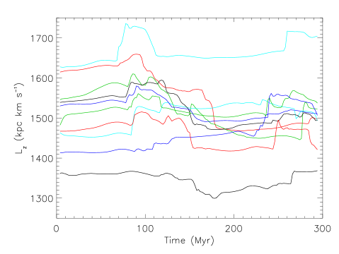
Figure 4: The angular momentum ($z$-component) with time of 10 selected particles with 6.8 kpc $<r<$ 7.8 kpc. The particles are initially all at the same azimuth, but at different radii.

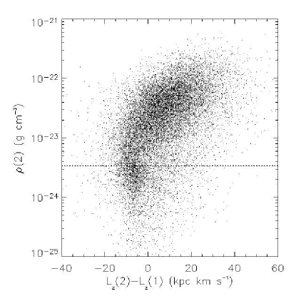
Figure 5: The jump is $z$-component of angular momentum ($L_{z}(2)-L_{z}(1)$) is plotted as a function of post-shock density ($\rho(2)$) for a number of particles. The pre-shock densities of the particles (not shown) all fall below the dotted line. There is a strong correlation between density enhancement in the shock and the magnitude of the jump in $L_{z}$.

Figure 6: The number of particles (N(L_z)) which have the value of the $z$ component of the angular momentum L_z. The total number of particles for the whole disk is included at the beginning of the simulation (solid line), after 140 Myr (dashed line) and after 280 Myr (dotted line).

Although the pre-shock ISM is inhomogeneous, we find that this clumpiness is amplified within the spiral arms. It is this amplification which gives rise to the structures within the arm (Figure 2), particularly in the molecular gas, as will be shown in Section 4.2. To see this in more detail, Figure 3 (upper) shows the distribution of particles in a small sector of our simulation. Since $\theta$ is measured clockwise round the disk, particles are located in the top part of the disk, and are selected to cover a spiral arm. Approaching the spiral arm from below can be seen apparent waves of material. These are in fact the remnants of clumps formed in the previous arm, by now strongly elongated by the differential shear in the inter-arm region (See Figure 2). These inhomogeneities, which are transmitted from the previous arm, provide input for new inhomogeneities in the next arm. In Figure 3 (lower) we plot the value of $L_{z}$ for each of the particles in Figure 3 (upper) as a function of the $\theta$-coordinate. The region below the arm in the upper Figure 3 now spans a relatively small range in $L_{z}$, and the phase-space density here is relatively smooth. Just above this is a region where the phase-space density drops. This corresponds to the rapid jump in $L_{z}$, discussed above, which occurs as particles enter the spiral shock. Above this we see a patchy structure of phase-space density enhancements. It is clear that the inhomogeneity which occurs here, within the arm, is much greater than that seen in the pre-shock gas.

The physical picture we have of what is happening here is as follows. We have seen that the gas, on entering the arm and being shocked, moves along the arm for a while (Roberts, 1969). It eventually leaves it to enter the inter-arm region, when its angular momentum is too high to follow the spiral arm to smaller radii. Imagine, then, as a simple model for the gas flowing along the arm, a set of masses flowing in a line along a smooth inclined tube under gravity. If the gas were all homogeneous, we would model this by adding masses to the tube at equal velocities, at a rate which is uniform in time and space. To mimic material leaving the arm, we remove masses from the tube at positions which depend on their velocity (for example, we could remove particles when their velocities exceed some particular value $V_{\max}$). In this case, at any one time the density of masses along the tube would remain smooth and independent of time. However, to model an inhomogeneous pre-shock ISM, we would add masses to the tube in a non-uniform manner in space, and with a range of velocities. In this case, as the masses move along the tube they would tend (assuming the encounters are dissipative) to bunch up, like traffic along a single lane highway. This bunching in velocity space can be seen in Figure 3 (lower). Since as before, we would remove masses from the tube at positions which depend on their velocities, it is clear that in this case, masses would not only tend to form clumps within the tube, but would also tend to be removed from the tube in clumps. As these clumps leave the spiral arms, they are sheared out to form the spurs and feathering seen in Figure 2.

Using these ideas we can obtain a rough estimate of the linear scale of the inhomogeneities we expect to find in the spiral arms. The typical time a particle spends within a spiral arm can be estimated from Figure 4 as being approximately $t_{arm}\sim 6\times 10^{7}$ years. The typical velocity spread of particles within a spiral arm can be seen from Figure 7 to be approximately $v_{\perp}\sim 10$ km s^-1. Then the average scale-length of density structure generated by the piling up process would be $L\sim t_{\rm arm}v_{\perp}\sim 600$ pc. This agrees roughly with the mean distance between the high-density peaks, most easily viewed from the molecular gas density (yellow) along the arm in Figure 9(iv).

Figure 7: The velocity dispersion plotted against azimuth ($\theta$, radians) for a ring whereby r=7.5 kpc and $\triangle$r=200 pc. The figure shows the dispersion of the $v_{\perp}=\sqrt{(v_{x}^{2}+v_{y}^{2})}$ (solid) and the dispersion of $v_{z}$ (dotted). ($\theta$ is measured clockwise round the disk, i.e. in the direction of gas flow). Insufficient resolution is likely to produce damping in the interarm regions. The figure corresponds to a time of 100 Myr in the simulation.

3.2 Velocity dispersion

In addition to introducing structure in the phase space density of the gas, spiral shocks can also induce large velocity dispersions in the gas (Bonnell et al., 2006). We determine the 2D velocity dispersion in the plane of the disk as a function of azimuthal angle. This is calculated by taking a 200 pc width ring centred at $r=7.5$ kpc. We divide this ring into 100 segments, each of length $r\triangle\theta=50$ pc and area $9\times 10^{4}$ pc² and calculate the velocity dispersion of the gas in each segment. Figure 7 shows the variation of the velocity dispersion for the 50 K simulation. The velocity dispersion is calculated after 100 Myr, for the velocity component in the plane of the galaxy, $v_{\perp}=\sqrt{(v_{x}^{2}+v_{y}^{2})}$, and the $z$ component of the velocity. There is a large increase of 10 km s^-1 in the dispersion of $v_{\perp}$ where the spiral arms occur. In comparison a velocity dispersion of 7-10 km s^-1 is observed for molecular clouds of sizes 20-50 pc (Solomon et al., 1987; Dame et al., 1986). Bonnell et al. (2006) find a velocity dispersion up to 10 km s^-1 in simulations of gas passing through a spiral shock. This velocity dispersion is due to random chaotic internal motions induced in clumpy gas subject to a shock. The velocity dispersion quickly decreases upon leaving the arms. A further decrease in the velocity dispersion occurs in the interarm regions. The ratio in the smoothing length compared to the disk scale height ($h/H$) approaches 1 in the interarm regions. This potentially leads to damping of velocities due to insufficient resolution, particularly in the $v_{z}$ velocity component.

4 Molecular gas

We have seen above that spiral shocks produce highly structured and dense gas that can be associated with molecular clouds in spiral arms. In addition, we would like to know whether such a formation mechanism is able to account for the formation of molecular gas from initially atomic gas or if such gas would need to be primarily molecular before entering the shock. In order to do this, we perform a rough estimate of the formation (and destruction) of molecular gas as the gas enters and leaves the spiral arms. We post-process the simulation by using the local gas properties determined by the isothermal simulations and calculate the time dependent formation rate of H₂ on dust grains as well as the dissociation rates by UV radiation and cosmic rays. At each time step from the simulation, the formation and destruction rate is calculated for each gas parcel (particle) and added to its previous molecular fraction. In this way, we can estimate the spatial and temporal evolution of the molecular gas throughout the simulation.

Since the gas in our models is isothermal, the formation of molecular hydrogen is not treated self-consistently. In particular there is no heating or cooling, as described in previous smaller scale analysis (Bergin et al., 2004; Audit & Hennebelle, 2005; Koyama & Inutsuka, 2000). As a first attempt to analyze the overall distribution of molecular hydrogen, and the densities required for H₂ formation, we post-process our results to find the time-dependent molecular density of gas in the disk. This is a simplistic approach but identifies the most dense gas in our simulations where molecular hydrogen forms. The reader should bear in mind however that heating from feedback and supernovae explosions will have some effect on these results.

We use a simple algorithm for the evolution of molecular hydrogen (Bergin et al., 2004) determined for molecular cloud formation behind shock waves. The rate of change of H₂ density is given by

$$\frac{dn(H_{2})}{dt}=R_{gr}(T)n_{p}n(H)-[\zeta_{cr}+\zeta_{diss}(N(H_{2}),A_{V})]n(H_{2})$$ (4)

where $n$ is the number density (of atomic or molecular hydrogen), $N$ is the column density (of atomic or molecular hydrogen) and T the temperature. The total number density is $n_{p}$, where $n_{p}=n(H)+2n(H_{2})$. Molecular hydrogen is produced through condensation onto grains, determined by the first term on the right of eqn(4). $R_{gr}$ is the formation rate on grains, which is proportional to T^0.5. The efficiency for the formation rate on grains is $S=0.3$ , although recent results suggest the efficiency is higher than this for temperatures of less than 90 K (Cazaux & Tielens, 2004). Destruction of H₂ occurs through cosmic ray ionization and photo-dissociation, represented by the second term on the right of eqn(4). The cosmic ionization rate, $\zeta_{cr}$ is assumed constant ($\zeta_{cr}=6\times 10^{-18}$ s^-1).

Following Bergin et al. (2004), we adopt the approximation of Draine & Bertoldi (1996) for the H₂ dissociation rate:

$$\begin{split}\zeta_{diss}(N(H_{2}))&=\zeta_{diss}f_{shield}(N(H_{2}))e^{-\tau_{d,1000}}\zeta_{diss}(0)\\ f_{shield}(N(H_{2}))&=\frac{0.965}{(1+x/3)^{2}}+\frac{0.035}{(1+x)^{0.5}}\\ &\times\exp[-8.5\times 10^{-4}(1+x)^{0.5}]\\ \text{where}\quad x&=N(H_{2})/5\times 10^{14}\text{cm}^{-2}\end{split}$$ (5)

The function $f_{shield}$ approximates the rate of photodissociation summed over all energy levels. Self shielding is included through the dependence on column density and $\tau_{d,1000}$ is the dust extinction at 1000 Å. The constant $\zeta_{diss}(0)=4.17\times 10^{-11}$ s^-1 is a measure of the strength of the UV field. This formulation assumes that the background UV spectrum is the same as that of a B0 star, and that the radiation flux is constant everywhere. The strength of the flux is measured by the magnitude of $\zeta_{diss}(0)$. We note that this is a very approximate measure of the the photodissociation rate, which should ideally vary depending on the local level of star formation. Furthermore, we only produce an estimate of the column density $N(H_{2})$ in our calculations by multiplying the local density by the scale height of the disk.

We divide Eqn(4) by $n_{p}$ and calculate the change in the molecular gas fraction, $d(n(H_{2})/n_{p})$, for each particle after each timestep (2 Myr). Assuming $n(H_{2})=0$ everywhere initially, we add the change in the molecular gas fraction to the ratio $n(H_{2})/n_{p}$ determined for the previous timestep. At each time frame, this ratio in the number densities can be converted to a volume density of molecular hydrogen. As shown in Figure 8, Eqn(4) mainly selects the most dense particles, although the molecular gas fraction is also time dependent. Since the formation of H₂ is not instantaneous, the molecular gas fraction increases with the time gas spends in the denser spiral arms.

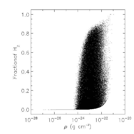
Figure 8: The distribution of the molecular fraction of particles is shown versus their density for the 50 K simulation, after 100 Myr. 1/10th of particles are plotted, i.e. $4\times 10^{5}$. There is a clear cut off at $n_{p}\thicksim 10^{-24}$ g cm^-3, below which the gas is totally atomic. The large spread in the H₂ fraction for a given density represents the time evolution of the H₂ fraction from when low density gas first enters the spiral shock.

4.1 Molecular gas formation at different temperatures

We find that H₂ formation in our simulations requires that the (isothermal) gas be cold, with temperatures of order 100 K or less. Of order 10% of the gas becomes molecular with these temperatures whereas when the gas is 1000 K the molecular fraction drops to around 1% and is virtually zero at $10^{4}$ K. We can thus conclude that the spiral shock formation of H₂ is likely when the ISM is cold. The fraction of molecular gas was found to decrease with lower resolution. For the 50 K highest resolution simulation, the total molecular gas in the disk reaches a maximum of $\sim 13\%$. The fraction of molecular gas was found to decrease with lower resolution. For 1 million particles, the amount of molecular hydrogen formed was very similar in the 10, 50 and 100 K cases, reaching a maximum of $\sim 8\%$ of the total mass.

The fact that the gas is assumed to be isothermal precludes a detailed study of the temperature dependency on H₂ formation as in reality this would depend on the details of the equation of state. For example, the efficiency of grain formation, assumed here to be a constant S=0.3, can be as high as S=1 for $T<20$ and as low as $S\sim 0.1$ for $T>100$ K (Cazaux & Tielens, 2004). What we can tell is that hot gas ($T\geq 1000$ K) does not form significant H₂ due to the shock dynamics.

When the gas is hot, the shock produced by the spiral potential is weaker, so the density of gas in the spiral arms is reduced. The density in the $10^{4}$ K simulation does not increase above $10^{-24}$ g cm^-3 which is too low for molecular hydrogen to form (Figure 8). The density of gas in the spiral arms is insufficient for self-shielding to occur and molecular gas is readily photodissociated. Similar conclusions were reached by Bergin et al. (2004), who require pressures a few times higher than the average interstellar values to allow effective self shielding. We do not include cooling, although for strong shocks performed at $10^{4}$ K (Koyama & Inutsuka, 2000) only a thin layer of molecular hydrogen forms. Therefore at higher temperatures, it is unlikely that spiral shocks could produce densities sufficient for significant molecular hydrogen formation.

4.2 High resolution simulation

In the remainder of the paper, we focus on the 50 K highest resolution simulation. We show the location of H₂ when the ISM temperature is 50 K in Figure 9. There are $4\times 10^{6}$ particles giving a mass resolution of 125 M_⊙ per particle. This figure is taken after 100 Myr, and shows the global distribution of molecular gas, and the small scale structure of molecular clouds.

Molecular hydrogen starts to form immediately in the spiral arms, the most dense parts of the disk. H₂ is first situated in a narrow strip, where the shock from the spiral density wave occurs. The density of gas leaving the arms is insufficient to prevent molecular gas quickly becoming photodissociated, hence the molecular gas is solely confined to the shock in the spiral arm. This strip of molecular hydrogen is smooth and continuous along the spiral arm. However, as the density of the shock increases, denser structures become apparent in the arms. These break up into separate clumps of molecular gas, which we identify as ’molecular clouds’. These molecular clouds are produced simply by the kinematics of the gas flowing in the spiral potential as described in Section 3.1, as self gravity is not included. As the simulation progresses, dense structures leaving the spiral arms become sheared. Some regions of molecular gas leaving the spiral arms are then dense enough for self shielding to reduce the rate of photodissociation. These molecular clouds survive further into the interarm regions.

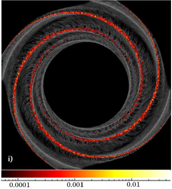
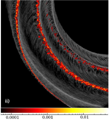
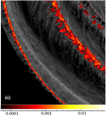
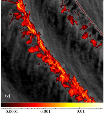
Figure 9: Column density plots (g cm^-2) showing density of molecular hydrogen (red) against overall density (black and white). Length-scales of plots are i) 20 kpc $\times$ 20 kpc, ii) 10 kpc $\times$ 10 kpc, iii) 5 kpc $\times$ 5 kpc (-8.5 kpc $<x<$ -3.5 kpc, -8.5 kpc $<y<$ -3.5 kpc), iv) 3 kpc $\times$ 3 kpc (-6.5 kpc $<x<$ -3.5 kpc, -6.5 kpc $<y<$ -3.5 kpc). The xy-coordinates assume a Cartesian grid centred on the midpoint of the disk which remains fixed with time. Gas is flowing clockwise across the disk.

4.3 Molecular gas and spiral structure

Figure 9 shows that molecular gas is largely confined to the denser spiral arms. We plot the average molecular and total (molecular and atomic) gas densities with azimuth in Figure 10, at 2 different times. As in Section 3.2, the densities are calculated from a ring centred at $r=7.5$ kpc divided into 100 segments. This plot only displays the mean molecular and atomic densities - the peak densities are 10-20 times higher. The interarm densities of H₂ are $10^{4}$ times smaller than in the spiral arms after 100 Myr, whilst the total densities are $\approx$ 50 times smaller. After 100 Myr, 10% of the gas in the ring is molecular. Approximately 70% of the total amount of gas is situated in the spiral arms, of which 20% is molecular. Figure 10 suggests that the existence of interarm molecular gas is unlikely, although we examine the effect of changing the disk mass and photodissociation rate next.

Figure 10: Density of molecular gas (solid) and total density (dotted) are plotted against azimuth ($\theta$), where $\theta$ (in radians) is the angle measured in the direction of flow. The density plotted is the average over an annulus centred at r=7.5 kpc with $\delta r$=200 pc. The time of the simulation is 100 Myr (top) and 290 Myr (bottom).

4.3.1 Dependence of H₂ formation on disk mass and photodissociation rate

The mass of H₂ in eqn (1) is determined by the density, photodissociation rate and temperature. The cosmic ray ionization rate, $\zeta_{cr}=6\times 10^{-18}$ s^-1, is found to have a minimal effect on the fraction of molecular to atomic gas. Since the H₂ mass is determined post process, calculations can be repeated with a different disk mass (as there is no self gravity) and/or different photodissociation rate. As expected, increasing the mass or decreasing the photodissociation rate considerably increase the formation of H₂. The mass of H₂ increases considerably to $1.4\times 10^{9}$ M_⊙, 28% of the total gas, when the disk mass increases by a factor of 10. In comparing with the photodissociation rate, the same approximation (eqn(4)) was applied, but increased or decreased by a constant factor. When the photodissociation rate decreases by a factor of 10, the molecular mass increases to $1.25\times 10^{8}$ M_⊙, 25% of the total gas mass.

The disk mass has a substantial effect on the arm-interarm fractional abundance of H₂. When the mass of the disk increases to $5\times 10^{9}$ M_⊙, nearly all the gas in the spiral arms is molecular at the end of the simulation (Figure 11). Whilst the interarm ratio of the total density to H₂ density also increases, only about 1/10th of the interarm gas is molecular. The increase in both the arm and interarm regions is due to higher densities increasing the formation of H₂.

The photodissociation rate has a more pronounced effect on the interarm ratios. When the photodissociation rate is a tenth of that taken from Draine & Bertoldi (1996), approximately a quarter of the interarm gas is molecular at the end of the simulation (Figure 11). By contrast the amount of H₂ in the spiral arms changes much less. This difference at a lower photodissociation rate arises when the gas is not fully dissociated between the spiral arms. Molecular gas can survive for longer into the interarm regions leading to some molecular structures between the arms. This is illustrated in Figure 12, which displays part of the 50 K simulation where the molecular gas density is calculated with the lower photodissociation rate. Clumps of molecular gas are shearing away from the spiral arm. In addition, molecular material is arriving at the spiral arm which has not fully dissociated from the previous spiral arm passage.

A more complete treatment of H₂ formation will give a more accurate idea of the quantitative analysis of molecular hydrogen (Glover & Mac Low, 2006a, b). Including heating may reduce the amount of molecular gas, but we defer commenting on the effects of feedback, and varying the photodissociation rate to depend on star formation to future studies. These results indicate nevertheless that the molecular gas is strongly confined to the spiral arms. The possibility that molecular hydrogen is transmitted between spiral arms cannot be ruled out though, e.g. if the photodissociation rate is sufficiently low. The effects of increasing the disk mass or decreasing the level of photodissociation are likely to hold when including heating and cooling of the gas.

Figure 11: Fractional abundance of H₂ in the arm (solid) and interarm regions (dashed) compared to the total disk mass (top) and photodissociation rate (bottom). These figures are taken from the end of the simulation.

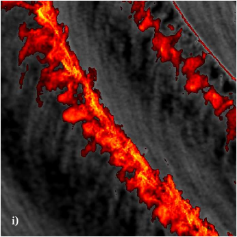
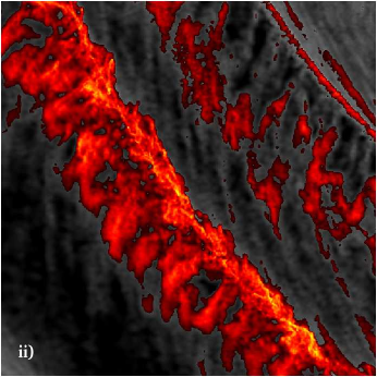
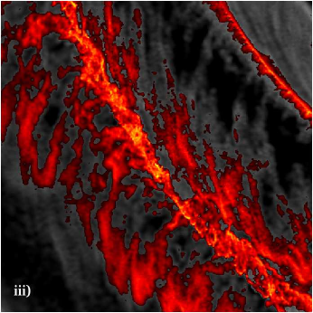
Figure 12: A 3 kpc by 3 kpc region of the disk showing the transfer of molecular hydrogen between spiral arms. The photodissociation rate is 1/10 that of Draine & Bertoldi (1996) and as a consequence, there is more molecular hydrogen surviving between the spiral arms. The column density of molecular hydrogen (red) and total density (black and white) are displayed (same scale as Figure 4). The times of each plot are i)100 Myr, ii)120 Myr and iii)140 Myr. Plot i) is the same time, region and scale as Figure 4(iv), but using a lower photodissociation rate. The increased density of H₂ along the arms leads to molecular structures within the interarm regions which are absent from the simulation in Figure 4.

5 Observational comparison of molecular cloud properties

One of the objectives of these simulations is to see how well the spiral shocks reproduce the observations of molecular clouds. We can directly compare our results with molecular clouds in the Milky Way. We consider the distribution of clouds from a local standard of rest comparable to the Sun, and a further LSR at the edge of the disk. Several surveys of molecular clouds in the Milky Way have been undertaken (e.g. Dame et al. 1986; Dame et al. 2001; Lee et al. 2001). We compare our data with 2 sets of results: i) the FCRAO CO survey of the outer galaxy (Heyer et al., 2001). This survey detected molecular clouds between the Galactic longitudes 102^o.49 and 141^o.54 which are located predominantly in the local and Perseus arms; ii) a CO molecular line survey (Yang et al., 2002), which detected cold infrared sources over the northern plane of the Galaxy (longitudes between 0^o and 260^o).

Our calculations give the fraction of molecular gas for each particle in the galactic disk. We use a simple algorithm to determine where molecular clouds are located. We select a section of 1/8 of the disk as a sample, and divide this region into a 5 pc resolution grid. We calculate the total fraction of molecular gas in each cell and retain cells which contain over 10 M_⊙ of H₂. We classify all groups of adjacent cells satisfying this threshold as a molecular cloud. The properties of each ’cloud’, including mass, position and velocity are tabulated. We determine the V_LSR of each molecular cloud - the locations of each LSR we have chosen are shown on Figure 13 compared to the overall distribution of molecular clouds.

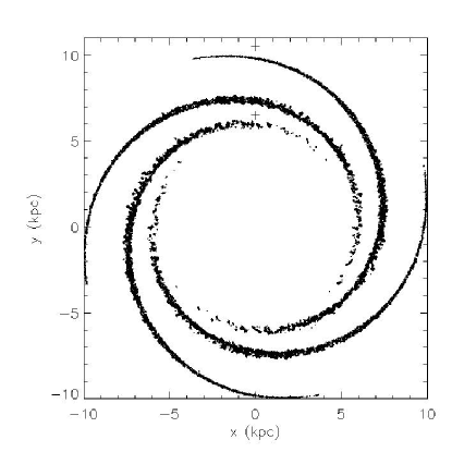
Figure 13: The position of each local standard of rest (crosses) is compared to the overall distribution of molecular clouds. The LSR situated at (0,6.5)kpc is comparable with the position of the Sun, in an interarm region in the mid-part of the disk. The second LSR (0,10.5)kpc produces a distribution of clouds as viewed from the edge of the disk.

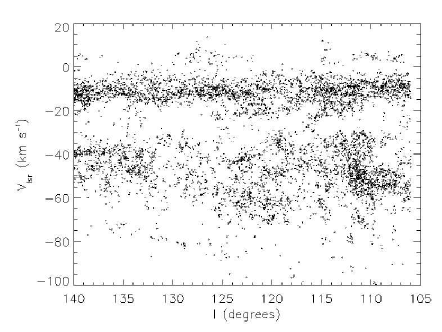
Figure 14: V_lsr plotted against galactic longitude for molecular clouds from these simulations and the FRCAO CO survey. The top plot shows the simulated data, with a LSR at coordinates (0,6.5)kpc. The lower plot uses data from the FCRAO CO survey (Heyer et al., 1998).

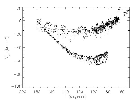
Figure 15: V_lsr plotted against galactic longitude for molecular clouds from these simulations and the CO molecular line survey. The top plot shows the simulated data, with a LSR at coordinates (0,6.5)kpc. The lower plot uses data from Yang et al. (2002).

In Figures 14 & 15, typical results from our calculations are compared with the FCRAO CO survey and the CO molecular line survey (where the LSR is situated at Cartesian coordinates (0,6.5)kpc). Our grid based method gave a total of 5044 objects within the sample criterion. Below these results corresponding data from the FCRAO CO survey are shown, where there are 7724 objects and the molecular line survey, where there are 1331 objects. The data from our model and the 2 surveys show clear bands, where the molecular clouds have preferential radial velocities due to the spiral arm structure. The molecular clouds in our model are more confined to the spiral arms than in the observational data, particular for the outer arm. We have assumed a corotation radius of 11 kpc, which may reduce the spiral arm shock at larger radii.

Figure 16 displays the molecular clouds as viewed from outside the disk, at coordinates (0,10.5)kpc. This is more comparable with Stark & Lee (2005), who observe clouds in the inner regions of the Milky Way. However their survey incorporates 5 spiral arms, whereas only 2 are clear in Figure 16.

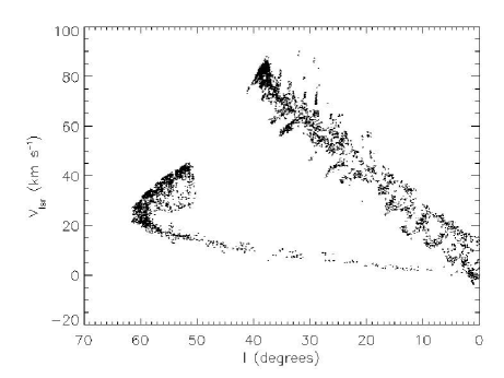
Figure 16: V_rms plotted against galactic longitude from simulated data. The LSR was chosen at coordinates (0,10.5)kpc

6 Conclusions

The simulations in this paper demonstrate the formation of molecular clouds in spiral galaxies, and specifically the role of spiral shocks. The compression as the gas passes through a spiral shock produces high density regions that are appropriate for the formation of molecular hydrogen. A necessary condition for this to occur is that the gas is cold ($T\lesssim 100$ K). Warm gas ($T\geq 1000$ K) produces little molecular hydrogen.

The spiral shock also produces significant structure in the gas along the arms. Cold gas is unstable to clumping in the shocks due to the semi-random encounters with lower and higher angular momentum gas. These denser structures are predominantly molecular and therefore identifiable as molecular clouds. An increased velocity dispersion is apparent in the spiral arms and thus molecular clouds, of similar magnitude to observations. We associate this increase in velocity dispersion with the generation of chaotic motions in the ISM as gas passes through clumpy shocks (Bonnell et al., 2006). We find only a small increase though in velocity dispersion in the vertical direction. Our simulations are not well resolved in the $z$ direction, and we would probably not expect to find high velocities in this direction without stellar energy injection (de Avillez & Breitschwerdt, 2005).

The total percentage of molecular hydrogen is typically $\sim 10\%$ for gas less than 100 K and a total disk gas mass of $5~{}\times 10^{8}$ M_⊙, (corresponding to a surface density of $\approx~{}2$ M_⊙ pc^-2), but this figure roughly doubles with a surface density of 20 M_⊙ pc^-2 or lower photodissociation rate. We note that these figures are potentially lower limits on the amount of molecular hydrogen formed in these models, since we find that the total percentage of molecular hydrogen increases with resolution. A caveat is that these results do not include realistic heating and cooling, which are likely to have some effect.

Since molecular gas formation is determined by density, and the time spent in dense regions, molecular gas is largely confined to the spiral arms. Typically we find the ratio of arm to interarm molecular hydrogen is 2 or 3 orders of magnitude. However a reduced photodissociation rate allows the survival of molecular gas into the interarm regions, and a ratio of arm to interarm molecular hydrogen less than 10. This leads to the possibility of molecular gas passing from one arm to the other and potentially determining subsequent molecular cloud formation.

The distribution of molecular clouds in our simulations is consistent with observational surveys of molecular clouds in the Milky Way. The confinement of molecular clouds to the spiral arms is more comparable to the outer Milky Way, where the ratio of arm to interarm clouds is high. The resolution is insufficient to gain accurate information about these clouds. Higher resolution simulations will determine whether the properties of individual molecular clouds (e.g. mass or internal velocity dispersion) can also be reproduced.

References

- Aannestad (1973) Aannestad P. A., 1973, ApJS, 25, 223
- Adler & Westpfahl (1996) Adler D. S., Westpfahl D. J., 1996, AJ, 111, 735
- Audit & Hennebelle (2005) Audit E., Hennebelle P., 2005, A&A, 433, 1
- Balbus (1988) Balbus S. A., 1988, ApJ, 324, 60
- Balbus & Cowie (1985) Balbus S. A., Cowie L. L., 1985, ApJ, 297, 61
- Benz (1990) Benz W., 1990, in in Buchler J.R., ed., Numerical Modelling of Nonlinear Stellar Pulsations Problems and Prospects, p269. Smooth Particle Hydrodynamics - a Review, Kluwer, Dordrecht
- Bergin et al. (2004) Bergin E. A., Hartmann L. W., Raymond J. C., Ballesteros-Paredes J., 2004, ApJ, 612, 921
- Binney & Tremaine (1987) Binney J., Tremaine S., 1987, Galactic dynamics. Princeton, NJ, Princeton University Press, 1987, 747 p.
- Blitz & Rosolowsky (2004) Blitz L., Rosolowsky E., 2004, ApJL, 612, L29
- Blitz & Williams (1999) Blitz L., Williams J. P., 1999, in Lada, C. J., Kylafis, N. D., eds, NATO ASIC Proc. 540: The Origin of Stars and Planetary Systems. Kluwer, Dordrecht, p3. Molecular Clouds
- Bonnell et al. (2006) Bonnell I. A., Dobbs C. L., Robitaille T. P., Pringle J. E., 2006, MNRAS, 365, 37
- Brouillet et al. (1998) Brouillet N., Kaufman M., Combes F., Baudry A., Bash F., 1998, A&A, 333, 92
- Brunt (2003) Brunt C. M., 2003, ApJ, 583, 280
- Caldwell & Ostriker (1981) Caldwell J. A. R., Ostriker J. P., 1981, ApJ, 251, 61
- Cazaux & Tielens (2004) Cazaux S., Tielens A. G. G. M., 2004, ApJ, 604, 222
- Clark & Bonnell (2004) Clark P. C., Bonnell I. A., 2004, MNRAS, 347, L36
- Clark et al. (2005) Clark P. C., Bonnell I. A., Zinnecker H., Bate M. R., 2005, MNRAS, 359, 809
- Cowie (1980) Cowie L. L., 1980, ApJ, 236, 868
- Cox & Gómez (2002) Cox D. P., Gómez G. C., 2002, ApJS, 142, 261
- Dame et al. (1986) Dame T. M., Elmegreen B. G., Cohen R. S., Thaddeus P., 1986, ApJ, 305, 892
- Dame et al. (2001) Dame T. M., Hartmann D., Thaddeus P., 2001, ApJ, 547, 792
- de Avillez & Breitschwerdt (2005) de Avillez M. A., Breitschwerdt D., 2005, A&A, 436, 585
- Digel et al. (1996) Digel S. W., Lyder D. A., Philbrick A. J., Puche D., Thaddeus P., 1996, ApJ, 458, 561
- Dobbs & Bonnell (2006) Dobbs C. L., Bonnell I. A., 2006, MNRAS, 367, 873
- Draine & Bertoldi (1996) Draine B. T., Bertoldi F., 1996, ApJ, 468, 269
- Dwarkadas & Balbus (1996) Dwarkadas V. V., Balbus S. A., 1996, ApJ, 467, 87
- Elmegreen (1979) Elmegreen B. G., 1979, ApJ, 231, 372
- Elmegreen (1982) Elmegreen B. G., 1982, ApJ, 253, 655
- Elmegreen (1989) Elmegreen B. G., 1989, ApJ, 344, 306
- Elmegreen (1990) Elmegreen B. G., 1990, in Blitz, L., ed., ASP Conf. Ser. 12: The Evolution of the Interstellar Medium. San Fracisco, p247.
- Elmegreen (1991) Elmegreen B. G., 1991, ApJ, 378, 139
- Elmegreen (1994) Elmegreen B. G., 1994, ApJ, 433, 39
- Elmegreen (2000) Elmegreen B. G., 2000, ApJ, 530, 277
- Elmegreen (2002) Elmegreen B. G., 2002, ApJ, 577, 206
- Elmegreen & Scalo (2004) Elmegreen B. G., Scalo J., 2004, ARA&A, 42, 211
- Engargiola et al. (2003) Engargiola G., Plambeck R. L., Rosolowsky E., Blitz L., 2003, ApJS, 149, 343
- Garcia-Burillo et al. (1993) Garcia-Burillo S., Guelin M., Cernicharo J., 1993, A&A, 274, 123
- Glover & Mac Low (2006a) Glover S. C. O., Mac Low M. ., 2006a, ArXiv Astrophysics e-prints
- Glover & Mac Low (2006b) Glover S. C. O., Mac Low M. ., 2006b, ArXiv Astrophysics e-prints
- Hartmann et al. (2001) Hartmann L., Ballesteros-Paredes J., Bergin E. A., 2001, ApJ, 562, 852
- Heyer et al. (1998) Heyer M. H., Brunt C., Snell R. L., Howe J. E., Schloerb F. P., Carpenter J. M., 1998, ApJS, 115, 241
- Heyer et al. (2001) Heyer M. H., Carpenter J. M., Snell R. L., 2001, ApJ, 551, 852
- Heyer & Terebey (1998) Heyer M. H., Terebey S., 1998, ApJ, 502, 265
- Hollenbach & McKee (1979) Hollenbach D., McKee C. F., 1979, ApJS, 41, 555
- Kaufman et al. (1999) Kaufman M. J., Wolfire M. G., Hollenbach D. J., Luhman M. L., 1999, ApJ, 527, 795
- Kennicutt (1989) Kennicutt R. C., 1989, ApJ, 344, 685
- Kim & Ostriker (2002) Kim W., Ostriker E. C., 2002, ApJ, 570, 132
- Koyama & Inutsuka (2000) Koyama H., Inutsuka S., 2000, ApJ, 532, 980
- Lee et al. (2001) Lee Y., Stark A. A., Kim H.-G., Moon D.-S., 2001, ApJS, 136, 137
- Li et al. (2005a) Li Y., Mac Low M., Klessen R. S., 2005a, ApJL, 620, L19
- Li et al. (2005b) Li Y., Mac Low M.-M., Klessen R. S., 2005b, ApJ, 626, 823
- Monaghan (1992) Monaghan J. J., 1992, ARA&A, 30, 543
- Monaghan & Lattanzio (1985) Monaghan J. J., Lattanzio J. C., 1985, A&A, 149, 135
- Monaghan & Lattanzio (1991) Monaghan J. J., Lattanzio J. C., 1991, ApJ, 375, 177
- Myers (1983) Myers P. C., 1983, ApJ, 270, 105
- Pringle et al. (2001) Pringle J. E., Allen R. J., Lubow S. H., 2001, MNRAS, 327, 663
- Rand & Kulkarni (1990) Rand R. J., Kulkarni S. R., 1990, ApJL, 349, L43
- Reddish (1975) Reddish V. C., 1975, MNRAS, 170, 261
- Reuter et al. (1996) Reuter H.-P., Sievers A. W., Pohl M., Lesch H., Wielebinski R., 1996, A&A, 306, 721
- Roberts (1969) Roberts W. W., 1969, ApJ, 158, 123
- Roberts & Stewart (1987) Roberts W. W., Stewart G. R., 1987, ApJ, 314, 10
- Scoville & Young (1983) Scoville N., Young J. S., 1983, ApJ, 265, 148
- Scoville & Hersh (1979) Scoville N. Z., Hersh K., 1979, ApJ, 229, 578
- Shu et al. (1987) Shu F. H., Adams F. C., Lizano S., 1987, ARA&A, 25, 23
- Shu et al. (1972) Shu F. H., Milione V., Gebel W., Yuan C., Goldsmith D. W., Roberts W. W., 1972, ApJ, 173, 557
- Solomon et al. (1987) Solomon P. M., Rivolo A. R., Barrett J., Yahil A., 1987, ApJ, 319, 730
- Tomisaka (1984) Tomisaka K., 1984, PASJ, 36, 457
- Vallée (2005) Vallée J. P., 2005, AJ, 130, 569
- Vogel et al. (1988) Vogel S. N., Kulkarni S. R., Scoville N. Z., 1988, Nature, 334, 402
- Wada & Koda (2004) Wada K., Koda J., 2004, MNRAS, 349, 270
- Wada et al. (2002) Wada K., Meurer G., Norman C. A., 2002, ApJ, 577, 197
- Wilson et al. (2005) Wilson B. A., Dame T. M., Masheder M. R. W., Thaddeus P., 2005, A&A, 430, 523
- Wolfire et al. (2003) Wolfire M. G., McKee C. F., Hollenbach D., Tielens A. G. G. M., 2003, ApJ, 587, 278
- Yang et al. (2002) Yang J., Jiang Z., Wang M., Ju B., Wang H., 2002, ApJS, 141, 157