Angular Trispectrum of CMB Temperature Anisotropy from Primordial Non-Gaussianity with the Full Radiation Transfer Function

Abstract

We calculate the cosmic microwave background (CMB) angular trispectrum, spherical harmonic transform of the four-point correlation function, from primordial non-Gaussianity in primordial curvature perturbations characterized by a constant non-linear coupling parameter, $f_{\rm NL}$. We fully take into account the effect of the radiation transfer function, and thus provide the most accurate estimate of the signal-to-noise ratio of the angular trispectrum of CMB temperature anisotropy. We find that the predicted signal-to-noise ratio of the trispectrum summed up to a given $l$ is approximately a power-law, $(S/N)(<l)\sim 2.2\times 10^{-9}f^{2}_{\rm NL}l^{2}$, up to the maximum multipole that we have reached in our numerical calculation, $l=1200$, assuming that the error is dominated by cosmic variance. Our results indicate that the signal-to-noise ratio of the temperature trispectrum exceeds that of the bispectrum at the critical multipole, $l_{c}\sim 1500~{}(50/|f_{\rm NL}|)$. Therefore, the trispectrum of the Planck data is more sensitive to primordial non-Gaussianity than the bispectrum for $|f_{\rm NL}|\gtrsim 50$. We also report the predicted constraints on the amplitude of trispectrum, which may be useful for other non-Gaussian models such as curvaton models.

Inflation has been the standard paradigm for the origin of cosmological fluctuations. While simple inflationary models based on a slowly-rolling scalar field are unable to generate the detectable level of primordial non-Gaussianity, a large class of models predict much stronger signals (see BKMR04 for a review). Non-Gaussianity of the primordial fluctuations thus plays an important role in testing and constraining inflationary models. As different statistical methods are sensitive to different aspects of non-Gaussianity, one should explore a variety of methods in order to maximize our sensitivity to primordial non-Gaussianity. Of which, the higher-order correlation functions such as the three- and four-point correlation functions, or their harmonic counterparts, the bispectrum KS01 ; K02 ; KSW05 ; BCZ04 ; BZ04 ; B05 ; L05 ; C05 and trispectrum KTHESIS ; KBCFG01 ; H01 ; OH02 , have been actively investigated in the literature as a powerful probe of primordial non-Gaussianity.

Compared with progress in theoretical calculations of the angular bispectrum of CMB temperature KS01 ; L05 and polarization BZ04 anisotropy, that for the angular trispectrum has been a little bit behind. The first calculation done by OH02 did not include the full effect of radiation transfer function caused by acoustic physics at the surface of last scatter. In this paper, we calculate the angular trispectrum of CMB temperature anisotropy, fully taking into account the radiation transfer function. Our estimate of the signal-to-noise ratio of the trispectrum should thus improve accuracy of the previous estimate based on an approximate method. We then compare the signal-to-noise ratios of primordial non-Gaussianity from the trispectrum and bispectrum.

Let us briefly review the formalism of the CMB angular trispectrum, following H01 ; OH02 . We decompose temperature anisotropy on the sky, $\delta T/T$, into spherical harmonic coefficients, $a_{lm}$, as

$$\frac{\delta T}{T}(\hat{\bm{n}})=\sum_{lm}a_{lm}Y_{lm}(\hat{\bm{n}}).$$ (1)

Statistical isotropy of the universe requires an $n$-point correlation function be rotationally invariant; thus, for $n=4$ one obtains

$$\langle a_{l_{1}m_{1}}a_{l_{2}m_{2}}a_{l_{3}m_{3}}a_{l_{4}m_{4}}\rangle=\sum_{LM}(-1)^{M}\left(\begin{array}[]{ccc}l_{1}&l_{2}&L\\ m_{1}&m_{2}&-M\end{array}\right)\left(\begin{array}[]{ccc}l_{3}&l_{4}&L\\ m_{3}&m_{4}&M\end{array}\right)T^{l_{1}l_{2}}_{l_{3}l_{4}}(L),$$ (6)

where $T^{l_{1}l_{2}}_{l_{3}l_{4}}(L)$ is the angular averaged trispectrum, $L$ is the length of a diagonal that forms triangles with $l_{1}$ and $l_{2}$ and with $l_{3}$ and $l_{4}$, and the matrix is the Wigner 3-$j$ symbol, which guarantees that two sides and the diagonal form a triangle, $|l_{1}-l_{2}|\leq L\leq l_{1}+l_{2}$ and $|l_{3}-l_{4}|\leq L\leq l_{3}+l_{4}$. Parity invariance also requires $l_{1}+l_{2}+L={\rm even}$, $l_{3}+l_{4}+L={\rm even}$, $m_{1}+m_{2}-M=0$, and $m_{3}+m_{4}+M=0$. These conditions determine the number of possible configurations.

The trispectrum generically consists of the connected, $T_{c}$, and unconnected, $T_{G}$, part:

$$T^{l_{1}l_{2}}_{l_{3}l_{4}}(L)=T_{c}{}^{l_{1}l_{2}}_{l_{3}l_{4}}(L)+T_{G}{}^{l_{1}l_{2}}_{l_{3}l_{4}}(L).$$ (7)

The former contains non-Gaussian signatures, while the latter contains only the angular power spectrum, $C_{l}\equiv\langle|a_{lm}|^{2}\rangle$,

$$T_{G}{}^{l_{1}l_{2}}_{l_{3}l_{4}}(L) = (-1)^{l_{1}+l_{3}}\sqrt{(2l_{1}+1)(2l_{3}+1)}C_{l_{1}}C_{l_{3}}\delta_{l_{1}l_{2}}\delta_{l_{3}l_{4}}\delta_{L0}$$ (8)

$$+(2L+1)C_{l_{1}}C_{l_{2}}\left[(-1)^{l_{1}+l_{2}+L}\delta_{l_{1}l_{3}}\delta_{l_{2}l_{4}}+\delta_{l_{1}l_{4}}\delta_{l_{2}l_{3}}\right].$$

Using permutation symmetry, one may write the connected part of the trispectrum as

$$T_{c}{}^{l_{1}l_{2}}_{l_{3}l_{4}}(L)=P^{l_{1}l_{2}}_{l_{3}l_{4}}(L)+(2L+1)\sum_{L^{\prime}}\left[(-1)^{l_{2}+l_{3}}\left\{\begin{array}[]{ccc}l_{1}&l_{2}&L\\ l_{4}&l_{3}&L^{\prime}\end{array}\right\}P^{l_{1}l_{3}}_{l_{2}l_{4}}(L^{\prime})+(-1)^{L+L^{\prime}}\left\{\begin{array}[]{ccc}l_{1}&l_{2}&L\\ l_{3}&l_{4}&L^{\prime}\end{array}\right\}P^{l_{1}l_{4}}_{l_{3}l_{2}}(L^{\prime})\right],$$ (13)

where

$$P^{l_{1}l_{2}}_{l_{3}l_{4}}(L)=t^{l_{1}l_{2}}_{l_{3}l_{4}}(L)+(-1)^{2L+l_{1}+l_{2}+l_{3}+l_{4}}t^{l_{2}l_{1}}_{l_{4}l_{3}}(L)+(-1)^{L+l_{3}+l_{4}}t^{l_{1}l_{2}}_{l_{4}l_{3}}(L)+(-1)^{L+l_{1}+l_{2}}t^{l_{2}l_{1}}_{l_{3}l_{4}}(L).$$ (14)

Here, the matrix is the Wigner 6-$j$ symbol, and $t^{l_{1}l_{2}}_{l_{3}l_{4}}(L)$ is called the reduced trispectrum, which contains all the physical information about non-Gaussian sources.

We parameterize primordial Bardeen’s curvature perturbation, $\Phi$, during the matter-dominated era in the usual form as KS01 ; OH02

$$\Phi(\bm{x})=\Phi_{\rm L}(\bm{x})+f_{\rm NL}\left[\Phi_{\rm L}^{2}(\bm{x})-\langle\Phi_{\rm L}^{2}(\bm{x})\rangle\right]+f_{2}\Phi_{\rm L}^{3}(\bm{x}),$$ (15)

where $\Phi_{\rm L}$ is the linear Gaussian part and $f_{\rm NL}$ and $f_{2}$ are the non-linear coupling parameters. (Note that $\Phi$ is a perturbation in the $(i,i)$-component of the metric.) The current observational constraint on $f_{\rm NL}$ is $-58<f_{\rm NL}<134$, which is from the analysis of the angular bispectrum of the WMAP data WMAPGAUSS1 ; WMAPGAUSS2 . No constraint on $f_{\rm NL}$ from the angular trispectrum is currently available. It is therefore important to obtain an accurate estimate of the signal-to-noise ratio of the angular trispectrum of primordial non-Gaussianity expected from the WMAP as well as Planck experiments PLANCK . While we take $f_{\rm NL}$ to be a constant independent of coordinates or wavenumbers, in general $f_{\rm NL}$ depends on scales, and different inflationary models predict different dependence of $f_{\rm NL}$ on wavenumbers BKMR04 . The post-inflationary evolution of $\Phi$ due to second-order metric perturbations, which must exist in any models of the standard cosmology, also generates wavenumber-dependent $f_{\rm NL}$ L05 . Nevertheless, a constant $f_{\rm NL}$ model is still useful for estimating sensitivity of CMB experiments to the amplitude of non-Gaussianity. Measurements of non-Gaussian fluctuations are usually quite challenging as non-Gaussianity is very small, which makes detection of wavenumber-dependent features even more challenging. Since currently there is no prediction for sensitivity of CMB experiments to $f_{\rm NL}$ from the angular trispectrum of CMB temperature anisotropy with the full radiation transfer function taken into account, we shall adopt a constant $f_{\rm NL}$ to explore the signal-to-noise ratio of the trispectrum as a function of the maximum multipoles measured by observations. In the future one may extend our approach to include scale-dependent $f_{\rm NL}$, following the method given in L05 , for instance.

The primordial fluctuations yield temperature anisotropy as

$$a_{lm}=4\pi(-i)^{l}\int\frac{d^{3}\bm{k}}{(2\pi)^{3}}\Phi(\bm{k})g_{Tl}(k)Y_{lm}^{*}(\hat{\bm{k}}),$$ (16)

where $g_{Tl}(k)$ is the radiation transfer function of adiabatic fluctuations, which can be calculated numerically by the CMBFAST code SZ96 . Using this relation, we obtain the formula of the reduced angular trispectrum as

$$t^{l_{1}l_{2}}_{l_{3}l_{4}}(L) = \int r_{1}^{2}dr_{1}r_{2}^{2}dr_{2}~{}F_{L}(r_{1},r_{2})\alpha_{l_{1}}(r_{1})\beta_{l_{2}}(r_{1})\alpha_{l_{3}}(r_{2})\beta_{l_{4}}(r_{2})h_{l_{1}Ll_{2}}h_{l_{3}Ll_{4}}$$ (17)

$$+\int r^{2}dr~{}\beta_{l_{2}}(r)\beta_{l_{4}}(r)\left[\mu_{l_{1}}(r)\beta_{l_{3}}(r)+\beta_{l_{1}}(r)\mu_{l_{3}}(r)\right]h_{l_{1}Ll_{2}}h_{l_{3}Ll_{4}},$$

where

$$F_{L}(r_{1},r_{2}) \equiv \frac{2}{\pi}\int k^{2}dk~{}P_{\Phi}(k)j_{L}(kr_{1})j_{L}(kr_{2}),$$ (18)

$$\alpha_{l}(r) \equiv \frac{2}{\pi}\int k^{2}dk~{}(2f_{\rm NL})g_{Tl}(k)j_{l}(kr),$$ (19)

$$\beta_{l}(r) \equiv \frac{2}{\pi}\int k^{2}dk~{}P_{\Phi}(k)g_{Tl}(k)j_{l}(kr),$$ (20)

$$\mu_{l}(r) \equiv \frac{2}{\pi}\int k^{2}dk~{}f_{2}g_{Tl}(k)j_{l}(kr),$$ (21)

and

$$h_{l_{1}Ll_{2}}\equiv\sqrt{\frac{(2l_{1}+1)(2l_{2}+1)(2L+1)}{4\pi}}\left(\begin{array}[]{ccc}l_{1}&l_{2}&L\\ 0&0&0\end{array}\right).$$ (24)

We have defined the power spectrum of the primordial curvature perturbation as

$$\langle\Phi_{\rm L}(\bm{k})\Phi_{\rm L}^{*}(\bm{k}^{\prime})\rangle=(2\pi)^{3}\delta^{(3)}(\bm{k}-\bm{k}^{\prime})P_{\Phi}(k),$$ (25)

where $P_{\Phi}\propto k^{n-4}$ and $n=1$ for a scale-invariant spectrum.

The signal-to-noise ratio of the temperature trispectrum is given by

$$\left(\frac{S}{N}\right)_{\rm tri}^{2}=\sum_{l_{1}>l_{2}>l_{3}>l_{4}}\sum_{L}\frac{[T_{c}{}^{l_{1}l_{2}}_{l_{3}l_{4}}(L)]^{2}}{(2L+1)C_{l_{1}}C_{l_{2}}C_{l_{3}}C_{l_{4}}}.$$ (26)

Note that we have assumed that the error is solely due to the cosmic variance. When detector noise is included, $C_{l}$ in the denominator should be replaced by $C_{l}+N_{l}/W_{l}$, where $N_{l}$ is the noisebias and $W_{l}$ is the window function. We set the normalization of $P_{\Phi}(k)$ by the height of the first acoustic peak of the WMAP data; $l(l+1)C_{l}/2\pi=(74.7{\rm\mu K})^{2}$ at $l=220$, and adopt the cosmological parameters of the concordance $\Lambda$CDM model with a scale-invariant primordial spectrum for $\Phi$; $h=0.72$, $\Omega_{b}=0.047$, $\Omega_{\Lambda}=0.71$, $\Omega_{m}=0.29$, and $\tau=0.17$ SPERGEL . While we shall evaluate $(S/N)^{2}$ using the trispectrum that uses the radiation transfer function [equation (17)] below, let us first estimate an order-of-magnitude of $(S/N)^{2}$ and its dependence on the maximum multipole, $l_{\rm max}$, using the Sachs–Wolfe approximation valid at low multipoles ($l\ll 100$), $g_{Tl}(k)\approx-j_{l}(kr_{*})/3$, where $r_{*}$ is the comoving distance to the surface of last scatter. This form of $g_{Tl}(k)$ then gives

$$t^{l_{1}l_{2}}_{l_{3}l_{4}}(L)\approx 9C_{l_{2}}^{\rm SW}C_{l_{4}}^{\rm SW}\left[4f_{\rm NL}^{2}C_{L}^{\rm SW}+f_{2}\left(C_{l_{1}}^{\rm SW}+C_{l_{3}}^{\rm SW}\right)\right]h_{l_{1}Ll_{2}}h_{l_{3}Ll_{4}},$$ (27)

where

$$C_{l}^{\rm SW}=\frac{2}{9\pi}\int k^{2}dkP_{\Phi}(k)j_{l}^{2}(kr_{*})=\frac{A}{l(l+1)},$$ (28)

is the angular power spectrum in the Sachs–Wolfe approximation for a scale-invariant primordial spectrum of $\Phi$, and $A\approx 6\times 10^{-10}$. For simplicity we take into account only the first terms in equations (13) and (14). Moreover, let us consider only $L=1$ modes because the collapsed configurations, which correspond to the low-$L$ modes, are the dominant modes for $f_{\rm NL}$ model [equation (15)]. This property also holds for the bispectrum BCZ04 ; C05 . For $f_{2}=0$ we have

$$t^{l_{1}l_{2}}_{l_{3}l_{4}}(L=1)\approx 36f_{\rm NL}^{2}C_{L=1}^{\rm SW}C_{l_{2}}^{\rm SW}C_{l_{4}}^{\rm SW}h_{l_{1},1,l_{2}}h_{l_{3},1,l_{4}}.$$ (29)

Since $|l_{1}-1|\leq l_{2}\leq l_{1}+1$ from the triangle condition and $l_{1}>l_{2}$, $h_{l_{1},1,l_{2}}$ is non-zero only for $l_{1}-1=l_{2}$. Hence

$$h_{l_{1},1,l_{2}}^{2} = \frac{3}{4\pi}(2l_{1}+1)(2l_{2}+1)\left(\begin{array}[]{ccc}l_{1}&l_{2}&1\\ 0&0&0\end{array}\right)^{2}$$

$$= \frac{3}{4\pi}(2l_{1}+1)(2l_{1}-1)\times\frac{l_{1}}{(2l_{1}-1)(2l_{1}+1)}\delta_{l_{1}-1,l_{2}}$$

$$= \frac{3l_{1}}{4\pi}\delta_{l_{1}-1,l_{2}},$$ (33)

which gives

$$\left(\frac{S}{N}\right)_{\rm tri}^{2} \approx \sum_{l_{1}>l_{2}>l_{3}>l_{4}}\frac{[t^{l_{1}l_{2}}_{l_{3}l_{4}}(L=1)]^{2}}{3C_{l_{1}}^{\rm SW}C_{l_{2}}^{\rm SW}C_{l_{3}}^{\rm SW}C_{l_{4}}^{\rm SW}}$$ (34)

$$\approx \left(\frac{27}{\pi}\right)^{2}\frac{1}{4!}\sum_{l_{1}l_{2}l_{3}l_{4}}\frac{f_{\rm NL}^{4}C_{l_{2}}^{\rm SW}C_{l_{4}}^{\rm SW}(C_{L=1}^{\rm SW})^{2}l_{1}l_{3}\delta_{l_{1}-1,l_{2}}\delta_{l_{3}-1,l_{4}}}{3C_{l_{1}}^{\rm SW}C_{l_{3}}^{\rm SW}}$$

$$\approx A^{2}f_{\rm NL}^{4}l_{\rm max}^{4},$$

where $l_{\rm max}$ is the maximum multipole. This result indicates that $(S/N)^{2}$ of the trispectrum strongly depends on both $f_{\rm NL}$ and $l_{\rm max}$, $(S/N)^{2}_{\rm tri}\propto(f_{\rm NL}l_{\rm max})^{4}$, which is stronger than that of the bispectrum, $(S/N)^{2}_{\rm bi}\propto(f_{\rm NL}l_{\rm max})^{2}$ KS01 . We have confirmed that $l_{\rm max}^{4}$ dependence still holds when all the terms (still in the Sachs–Wolfe approximation) are included. The constant of proportionality is however about 20 times larger than equation (34). This is because there are other 11 terms due to the permutation symmetry as seen in equations (13) and (14), and summing over $L>1$ modes further increases $(S/N)^{2}$ by a factor of two. We shall show below that $l_{\rm max}^{4}$ dependence also holds very well for the full calculations.

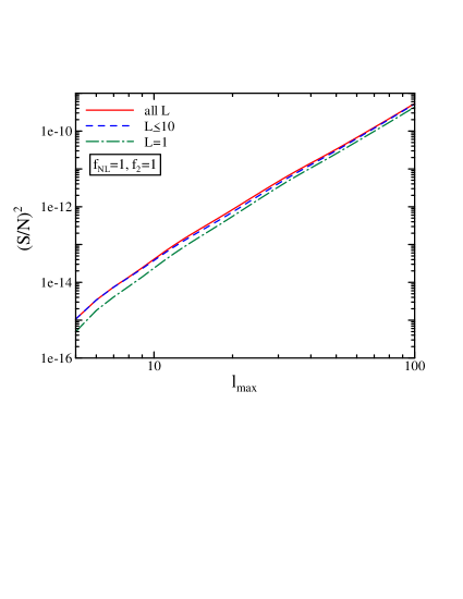
Figure 1: Signal-to-noise ratio squared, $(S/N)^{2}$, of the angular trispectrum summed over all $L$, $L\leq 10$, and only $L=1$ modes, respectively, as a function of the maximum multipole, $l_{\rm max}$. Here, $L$ denotes the multipole of the diagonal of a trispectrum configuration. We assume $f_{\rm NL}=1$ and $f_{2}=1$ and use the full radiation transfer function. This figure shows that the summation over $L$ needs to be done only up to $L\simeq 10$.

As the trispectrum calculation involves the summation over five multipoles, computation takes too long to let us go beyond $l_{\rm max}\sim 100$; however, we find that almost all the contribution actually comes from $L\lesssim 10$ as shown in Fig. 1 where we use the full radiation transfer function. It is therefore sufficient to perform the summation over the diagonal, $L$, only up to 10, which makes the computational time scale as $l_{\rm max}^{4}$ instead of $l_{\rm max}^{5}$, giving a huge saving in computational time. Figure 2 shows the predicted signal-to-noise ratio squared, $(S/N)^{2}$, for the trispectrum (summed over $L\leq 10$) as well as the bispectrum as a function of the maximum multipole, $l_{\rm max}$, with the full radiation transfer function. We have assumed a fiducial value of $f_{\rm NL}=50$ and $f_{2}=1$ in which case the effect of $f_{2}$ is negligible. Our result suggests that the expected signal-to-noise ratio of the primordial trispectrum is approximately given by

$$\left(\frac{S}{N}\right)^{2}_{\rm tri}\simeq 5\times 10^{-18}~{}f_{\rm NL}^{4}l_{\rm max}^{4},$$ (35)

or $(S/N)_{\rm tri}\simeq 2.2\times 10^{-9}~{}(f_{\rm NL}l_{\rm max})^{2}$. The minimum detectable $f_{\rm NL}$ by the trispectrum at the 1-$\sigma$ level is therefore $f_{\rm NL}\simeq 85$, 42, 21, 14, and 11 for $l_{\rm max}=250$, 500, 1000, 1500, and 2000. This may be compared with the minimum detectable $f_{\rm NL}$ by the bispectrum, $f_{\rm NL}\simeq 23$, 12, 6, 4, and 3 for $l_{\rm max}=250$, 500, 1000, 1500, and 2000. (Note again that we assume that the CMB bispectrum and trispectrum are cosmic-variance limited up to $l_{\rm max}$.) Here, we have used a power-law fit to $(S/N)_{\rm bi}\simeq 1.7\times 10^{-4}~{}|f_{\rm NL}|l_{\rm max}$. The power-law fits must break down at $l_{\rm max}\gtrsim 3000$, where $(S/N)^{2}$ does not grow due to the gravitational lensing effects increasing the cosmic variance KS01 ; BZ04 .

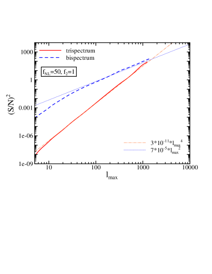
Figure 2: Predicted signal-to-noise ratio squared, $(S/N)^{2}$, of the angular trispectrum and bispectrum with the full radiation transfer function for $f_{\rm NL}=50$ and $f_{2}=1$. Power-law fits are also shown. Note that the power-law fits break down at $l_{\rm max}\gtrsim 3000$, where the gravitational lensing effects become important: $(S/N)^{2}$ ceases to grow at $l_{\rm max}\sim 3000$ KS01 ; BZ04 .

These results might seem to imply that the temperature trispectrum is always less sensitive to $f_{\rm NL}$ than the bispectrum; however, as $(S/N)_{\rm tri}$ depends on $f_{\rm NL}$ more strongly than $(S/N)_{\rm bi}$, the ratio also depends on $f_{\rm NL}$:

$$\frac{(S/N)_{\rm tri}}{(S/N)_{\rm bi}}\simeq\frac{|f_{\rm NL}|}{52}\frac{l_{\rm max}}{1500}.$$ (36)

The trispectrum actually becomes more sensitive to primordial non-Gaussianity than the bispectrum for Planck-like experiments probing $l_{\rm max}\gtrsim 1500$ and $|f_{\rm NL}|\gtrsim 50$. Incidentally, the trispectrum cannot measure the sign of $f_{\rm NL}$, as it depends on $f_{\rm NL}^{2}$. While we have considered the trispectrum of temperature anisotropy only, the signal-to-noise ratio should increase when polarization is included in the analysis. The number of possible combinations of the temperature and $E$-polarization field for the trispectrum is 5, while that for the bispectrum is 4; thus, one expects similar improvements in the signal-to-noise ratio for the bispectrum and trispectrum. The calculation including the temperature and polarization bispectra has shown that the signal-to-noise ratio increases roughly by a factor of 2 BZ04 . We expect a similar level of improvement for the trispectrum as well.

Equation (36) holds only for the particular non-Gaussian model given by equation (15); however, the amplitude of the trispectrum may be related to that of the bispectrum in a very different way for other models. For example, the curvature perturbation may be given by

$$\Phi(\bm{x})=\Phi_{\rm L}(\bm{x})+f_{\eta}\left[\eta^{2}(\bm{x})-\langle\eta^{2}(\bm{x})\rangle\right],$$ (37)

instead of equation (15), where $\eta$ is another fluctuating field that is totally uncorrelated with $\Phi_{\rm L}$. This form of non-Gaussianity may arise from a particular configuration of curvaton models LM97 ; LUW03 . (The form of the CMB angular bispectrum arising from this model has been derived in Appendix C of KTHESIS .) In this model the ratio of the amplitude of trispectrum to bispectrum is very different from that for equation (15). Boubekeur and Lyth BL06 proposed to use the following parameterization for the trispectrum amplitude of primordial curvature perturbation in the comoving gauge, $\zeta$, which is related to Bardeen’s curvature perturbation during the matter era as $\zeta=(5/3)\Phi$:

$$\langle\zeta(\bm{k}_{1})\zeta(\bm{k}_{2})\zeta(\bm{k}_{3})\zeta(\bm{k}_{4})\rangle=(2\pi)^{3}\delta^{(3)}(\bm{k}_{1}+\bm{k}_{2}+\bm{k}_{3}+\bm{k}_{4})\tau_{\rm NL}\left[P_{\zeta}(k_{1})P_{\zeta}(k_{2})P_{\zeta}(|\bm{k}_{1}+\bm{k}_{4}|)+(11~{}{\rm distinct~{}permutations})\right].$$ (38)

Equation (15) with $f_{2}=0$ gives $\tau_{\rm NL}=(6f_{\rm NL}/5)^{2}$, while equation (37) gives different predictions BL06 . Our results therefore give the minimum detectable $\tau_{\rm NL}$ at the 1-$\sigma$ level as $\tau_{\rm NL}\simeq 10400$, 2500, 640, 280, and 170 for $l_{\rm max}=250$, 500, 1000, 1500, and 2000. These results should be useful for estimating sensitivity of CMB experiments to a variety of non-Gaussian models giving rise to non-zero trispectrum.

Our predictions show that the angular trispectrum measured from WMAP is unable to detect primordial non-Gaussianity parameterized by $f_{\rm NL}$ as in equation (15), given the current constraint on $f_{\rm NL}$ from the bispectrum. However, the trispectrum is at least as powerful as the bispectrum for detecting primordial non-Gaussianity in the Planck data if $|f_{\rm NL}|\sim 50$, which is still allowed by the WMAP data. For other models, no detection of significant trispectrum on the WMAP ($l_{\rm max}\sim 250$) and Planck data ($l_{\rm max}\sim 1500$) would imply $\tau_{\rm NL}\lesssim 2\times 10^{4}$ and 560 at the 2-$\sigma$ level, respectively.

References

• (1) N. Bartolo, E. Komatsu, S. Matarrese and A. Riotto, Phys. Rept. 402, 103 (2004)
• (2) E. Komatsu and D. N. Spergel, Phys. Rev. D 63, 063002 (2001)
• (3) E. Komatsu, B. D. Wandelt, D. N. Spergel, A. J. Banday and K. M. GΓ³rski, Astrophys. J. 566, 19 (2002)
• (4) E. Komatsu, D. N. Spergel and B. D. Wandelt, Astrophys. J. 634, 14 (2005)
• (5) D. Babich, P. Creminelli and M. Zaldarriaga, JCAP 0408, 009 (2004)
• (6) D. Babich and M. Zaldarriaga, Phys. Rev. D 70, 083005 (2004)
• (7) D. Babich, Phys. Rev. D 72, 043003 (2005)
• (8) M. Liguori, F. K. Hansen, E. Komatsu, S. Matarrese and A. Riotto, Phys. Rev. D, in press (astro-ph/0509098)
• (9) P. Cabella, F. K. Hansen, M. Liguori, D. Marinucchi, S. Matarrese, L. Moscardini and N. Vittorio, preprint (astro-ph/0512112)
• (10) E. Komatsu, PhD Thesis, Tohoku University (2001) (astro-ph/0206039)
• (11) M. Kunz, A. J. Banday, P. G. Castro, P. G. Ferreira and K. M. Gorski, Astrophys. J. 563, L99 (2001)
• (12) W. Hu, Phys. Rev. D 64, 083005 (2001)
• (13) T. Okamoto and W. Hu, Phys. Rev. D 66, 063008 (2002)
• (14) E. Komatsu et al., Astrophys. J. Suppl. 148, 119 (2003)
• (15) P. Creminelli, A. Nicolis, L. Senatore, M. Tegmark and M. Zaldarriaga, preprint (astro-ph/0509029)
• (16) Planck website; http://www.rssd.esa.int/index.php?project=PLANCK
• (17) U. Seljak and M. Zaldarriaga, Astrophys. J. 469, 437 (1996)
• (18) D. N. Spergel et al., Astrophys. J. Suppl. 148, 175 (2003)
• (19) A. Linde and V. Mukhanov, Phys. Rev. D 56, R535 (1997)
• (20) D. H. Lyth, C. Ungarelli and D. Wands, Phys. Rev. D 67, 023503 (2003)
• (21) L. Boubekeur and D. H. Lyth, preprint (astro-ph/0504046)