Accurate photometry of extended spherically symmetric sources

We present a new method to derive reliable photometry of extended spherically symmetric sources from HST images (WFPC2, ACS/WFC and NICMOS/NIC2 cameras), extending existing studies of point sources and marginally resolved sources. We develop a new approach to accurately determine intrinsic sizes of extended spherically symmetric sources, such as star clusters in galaxies beyond the Local Group (at distances $\lesssim 20$ Mpc), and provide a detailed cookbook to perform aperture photometry on such sources, by determining size-dependent aperture corrections (ACs) and taking sky oversubtraction as a function of source size into account.
In an extensive Appendix, we provide the parameters of polynomial relations between the FWHM of various input profiles and those obtained by fitting a Gaussian profile (which we have used for reasons of computational robustness, although the exact model profile used is irrelevant), and between the intrinsic and measured FWHM of the cluster and the derived AC. Both relations are given for a number of physically relevant cluster light profiles, intrinsic and observational parameters. AC relations are provided for a wide range of apertures. Depending on the size of the source and the annuli used for the photometry, the absolute magnitude of such extended objects can be underestimated by up to 3 mag, corresponding to an error in mass of a factor of 15.
We carefully compare our results to those from the more widely used DeltaMag method, and find an improvement of a factor of 3–40 in both the size determination and the AC.

1 Introduction

We present a new method to determine photometric properties of extended spherically symmetric sources in Hubble Space Telescope (HST) data obtained with the Wide Field and Planetary Camera 2 (WFPC2), the Advanced Camera for Surveys / Wide Field Camera (ACS/WFC), and camera 2 of the Near Infrared Camera and Multi Object Spectrometer (NICMOS).

When studying extragalactic star clusters (SCs) at high spatial resolution, such as with the HST, the accuracy of “classical” photometric methods becomes insufficient. Ideally, fitting the point-spread functions (PSFs) is desirable for sources in crowded fields and with variable background fluxes. However, this is difficult since SCs at distances of $\lesssim$ 20 Mpc appear extended on the HST images and, as a consequence, PSF fitting techniques will underestimate their true fluxes.

With the best spatial resolution possible to achieve today ($\sim 0.05$ arcsec with the HST, namely using WFPC2/PC, ACS/WFC and ACS/HRC) many nearby clusters are clearly resolved. We define a “clearly resolved” cluster conservatively as having 1.2 $\times$ the PSF size, and hence an observed cluster FWHM roughly of the order of 2.3 pixels (see Table 3). As will be shown below, these 2.3 pixel correspond to an intrinsic cluster FWHM on the order of 0.5 pixel.

In addition, the high spatial resolution of the WFPC2 and ACS cameras undersample the PSF. For marginally extended sources, a satisfactory solution to this undersampling problem has recently been included in the HSTphot PSF fitting software package custom-written to handle HST photometry (Dolphin 2000).

Measuring the light in a fixed annulus around the central source coordinates, as commonly done in aperture photometry, can in principle correct for both the undersampled PSF and source size. However, when studying a population of sources with variable sizes, as for extragalactic SC systems in general, using a fixed aperture will underestimate the flux of the larger sources with respect to that of the point-like sources.

Many extragalactic SC studies have tried to estimate the size of the sources based on the magnitude difference in different apertures (we will refer to this as the “DeltaMag method”), and compare these to either model clusters (usually assuming Gaussian light profiles; e.g. Whitmore et al. 1993; Whitmore & Schweizer 1995; Zepf et al. 1999) and/or observed star profiles (e.g. Zepf et al. 1999). Sometimes, multiple apertures and cumulative light distributions are used, thus enhancing reliability (e.g. Puzia et al. 1999). However, as shown in de Grijs et al. (2001), the presence of a variable, structured background strongly compromises the results from the DeltaMag method.

In the same studies, estimates of aperture corrections (ACs) needed to account for the finite size of the objects are given, again on the basis of either model clusters (e.g. Whitmore & Schweizer 1995) or isolated clusters in the science images of interest (e.g. Miller et al. 1997; Carlson et al. 1998), mostly determined for a subset of clusters and applied to the whole sample – independent of object size. Some authors do attempt to use size-dependent ACs (e.g. Zepf et al. 1999), although generally not well defined, and mostly based on the rough size estimates resulting from the magnitude difference method. This method is vulnerable to centering problems (the use of 0.5 pixel radius apertures is seen regularly), and the sizes (and derived size-dependent ACs, as a consequence) are only rough estimates.

Other studies are based on more subjective methods, such as those that determine the source and sky annuli for each cluster individually, to encircle the dominant cluster light contribution and to avoid background contamination (see e.g. de Grijs et al. 2001; Anders et al. 2004). While this method avoids ACs (since it is already supposed to measure the dominant light contribution), it is hampered by subjectivity, and does not provide reliable size estimates.

There exist, as yet, no large-scale theoretical studies of the reliability, reproducibility and comparability of the results for any of these methods. All are subject to subjectivity in one aspect or another (e.g. the choice of apertures for size estimates/photometry, cluster light profile, selection of a few single clusters to derive “average” ACs).

To date, only two sophisticated systematic studies have been done to determine accurate SC sizes:

• Carlson & Holtzman (2001), but limited to marginally resolved, high S/N sources, without studying the accompanying ACs

• Dolphin & Kennicutt (2002) related to the above-mentioned program package HSTphot and its application to (again) marginally resolved sources in NGC 3627. This study is based on a PSF-fitting strategy for extended sources, while our work is based on aperture photometry.

The present study complements, expands upon and enhances those of Carlson & Holtzman (2001) and Dolphin & Kennicutt (2002). This study also fully complements structural studies of resolved clusters, e.g. in the Large and Small Magellanic Clouds (LMC, SMC) and nearby dwarf galaxies (see e.g. Mackey & Gilmore 2003a,b). However, such studies are only possible for the very nearest galaxies and their clusters. Where ACs are concerned, this study extends the widely-used work of Holtzman et al. (1995) for point sources to the studies of extended spherically symmetric sources.

In this paper, we present a new method to perform more accurate aperture photometry of extended spherically symmetric sources using a simple extension to the basic principle of aperture photometry. After measuring the flux of each source using a fixed aperture size, a variable AC (based on the actual size of the object) is applied. This method greatly enhances reproducibility and comparability of the results obtained. With the large range of parameter space explored and numerous related effects taken into account, we also present for the first time a method to estimate uncertainties in the sizes and ACs for a given observation.

In Section 2 we propose a general definition of “size”, as a function of a large number of intrinsic and observational parameters. In Section 3 the relation between source FWHM and the appropriate AC is determined as a function of aperture size. In Section 4 we provide a detailed “cookbook”, ready for immediate application to extragalactic SC systems. The reader who is only interested in applying our ACs could skip directly to Section 4. In Section 5 we provide an example error analysis for our new method, including a comparison of the method presented here to the DeltaMag method.

2 Determining accurate source sizes

Conventionally, the stellar density distributions of old globular clusters (GCs) are well described by King profiles (King 1962) with a range of concentration parameters. Intermediate-age and young star clusters (YSCs), e.g., in the LMC, are better described by Elson, Fall & Freeman (1987; EFF) profiles. Such clusters, similar to YSCs in, e.g., the Antennae galaxies or NGC 7252, do not (yet) show evidence of tidal truncations, in contrast to King profiles. We set out to analyse SC systems containing SCs spanning a large range of ages, masses and sizes, and compare radii and compactnesses of SCs in different galaxies. We therefore need a reliable method to estimate, to high accuracy, the radii of a large variety of SCs.

Thus, we first have to find a general definition of “size”. To this end, we created artificial SCs based on a variety of profiles using the BAOlab package of Larsen (1999) (for recent applications see Larsen 2004a; Boeker et al. 2004). BAOlab creates artificial clusters of a given magnitude by randomly drawing the position of each recorded photon from the input light profile. It thus simulates the stochastic nature of real observations very effectively, indeed more effectively than any other program available. These profiles were convolved with pre-calculated PSFs, generated with the Tiny Tim package (Krist & Hook 2004), and (for WFPC2 and ACS/WFC) the appropriate diffusion kernels supplied by Tiny Tim. Although some caveats still exist, Tiny Tim is the best suited package to obtain realistic HST PSFs to date. First, it extensively covers the parameter space of interest (cameras, filters, chips, position on the chips, object spectra, focus, PSF sizes etc.), well beyond anything that can be realisticly done with observed PSFs. And secondly, and even more crucial, the subsampling of Tiny Tim PSFs allows one to study the real distribution of counts onto adjacent pixels, depending on the exact PSF peak position on subpixel basis. This subsampling is fully implemented and used in the BAOlab package.

In order to measure the size of these objects we fit Gaussian profiles to them. Many extragalactic SC systems observed to date display a wide range of cluster sizes, so that we need to have a consistent and robust size determination to compare SC sizes and compactnesses. Therefore, we decided to apply a blanket fitting approach of Gaussian profiles to the SC light distributions. We realise that this is a simplification, but fitting more complicated profiles (such as King or EFF profiles) requires high signal-to-noise (S/N) ratios and the knowledge of whether or not the clusters are tidally truncated. In practice, this will be difficult for a large number of sources in realistic SC samples. We point out that the actual, underlying cluster profile is only of minor importance for the relative size determinations of SCs in a given SC system; the key prerogative is that one applies a consistent approach to one’s size determinations. Since we also base our ACs on such Gaussian fits our approach is fully internally consistent, and we have, in effect, taken the detailed profile shape out of the equation. In Sections 2.1 to 2.7 we will perform a detailed analysis for the WFPC2 camera. In Section 2.8 and 2.9 we will expand this to the ACS/WFC and NICMOS/NIC2 cameras.

Finally, we note that fitting more realistic light profiles results in less stable fit results, since either King or EFF profiles have one additional free parameter (concentration and power-law slope, respectively). They are also more sensitive to features at the periphery of the cluster, i.e., in the low-S/N regions.

Throughout this paper, we will use the FWHM of the input profile and the measured FWHM of the fitted Gaussian profile as measures for the size. In Table 1 we present the (constant) conversion factors from FWHM to the more widely used half-light radius, $R_{1/2}$, for the different models (e.g., Larsen 2004b).

2.1 The parameters of the “standard” cluster

In the following subsections we will investigate the behaviour of the measured cluster sizes (using the FWHM of a Gaussian profile, as justified in the previous section) as a function of the input FWHM, assuming various parameters for the artificial clusters and a range of observational conditions. In the Appendices we provide conversion relations between input and measured FWHM (and vice versa), by fitting fifth-order polynomials to these conversion relations, of the form

$${\rm size}(x)=a+b*x+c*x^{2}+d*x^{3}+e*x^{4}+f*x^{5}$$ (1)

and

$${\rm size}^{\prime}(y)=a^{\prime}+b^{\prime}*y+c^{\prime}*y^{2}+d^{\prime}*y^{3}+e^{\prime}*y^{4}+f^{\prime}*y^{5}$$ (2)

where $x$ and size${}^{\prime}(y)$ are the intrinsic FWHM in pixels, and size$(x)$ and $y$ the measured FWHM. We decided to use fifth-order polynomials after a visual inspection of the data and the fit results, as a compromise between fitting details in the shape, wiggles and instabilities in the fits, and usability. We note that this choice is purely based on mathematical convenience, and not on any physical properties of the SCs.

We first define our “standard” cluster:

• “Observations”: cluster of mag(WFPC2/F555W $\approx V)=10$ mag, observed in a 1s exposure;

• Tiny Tim PSF properties: HST WFPC2/WF3 chip; central position on the chip, i.e., $(x,y)=(400,400)$; F555W filter; using standard WFPC2 diffusion kernel;

• BAOlab parameters: no noise, profile fitting radius = 5 pixels; used for cluster generation and cluster fitting;

• Input cluster light profiles: Gaussian; King (1962) models with concentrations $c=5,30,100$ ; Elson et al. (1987) models with power-law index $\gamma=1.5,2.5$ (cf. Section 2.2);

• Fit model: Two-dimensional (2D) Gaussian profile, without taking into account any Tiny Tim HST PSF or HST diffusion kernel (effectively using a delta function-type PSF).

Although in the following sections we will plot the conversion relations for a larger range of input FWHMs (in order to illustrate that we understand their behaviour across the entire range of realistic sizes), we strongly advise to use these relations only in the range of $0.5\leq$ input FWHM (pixels) $\leq 10$. For smaller input FWHM, the data are not well approximated by the fitted polynomials. For larger input FWHMs, the S/N ratio per pixel decreases, and as a consequence the noise increases, so that the fit will not be sufficiently accurate. In other words, after converting measured radii to “intrinsic” radii, it is advisable to treat clusters with “intrinsic” radii outside the 0.5 – 10 pixel range with caution.

2.2 Size determination as a function of input model

In this Section we use the “standard” clusters defined in Section 2.1. The models used are a Gaussian model, King (1962) models with $c=$ 5, 30 and 100 (King 5, King 30 and King 100, respectively), and EFF profiles (Elson et al. 1987) with power-law indices $\gamma=$ 1.5 and 2.5 (EFF 15 and EFF 25, respectively). We point out that the power-law index $\gamma$ used in BAOlab differs by a factor of 2 from the definition used by Elson et al. (1987), with $\gamma_{\rm EFF}=2\times\gamma_{\rm BAOlab}$.

The light profiles are represented by the following equations, where $r$ is the (dimensionless) radius (in units of FWHM), and $w$ is a (dimensionless) normalisation constant:

• Gaussian:

  $$f(r)=\exp\left(-\left(r\cdot w\right)^{2}\right),$$ (3)

  with $w=2\sqrt{\ln(2)}\approx 1.66$

• King models:

  $$f(r,c)=\left(\frac{1}{\sqrt{1+\left(r\cdot w\right)^{2}}}-\frac{1}{\sqrt{1+c^{2}}}\right)^{2},$$ (4)

  with $w=2\sqrt{\left(\sqrt{0.5}+\frac{1-\sqrt{0.5}}{\sqrt{1+c^{2}}}\right)^{-2}-1}$, so that $w\approx 1.69,1.95$ and 1.98 for King 5, King 30 and King 100, respectively.

• EFF models:

  $$f(r,\gamma)=\left(1+\left(r\cdot w\right)^{2}\right)^{-\gamma},$$ (5)

  with $w=2\sqrt{2^{1/\gamma}-1}$, i.e., $w\approx 1.53$ and 1.13 for EFF 15 and EFF 25, respectively.

Table 1: Conversion factors to calculate a model’s $R_{\rm eff}=R_{1/2}$ from its FWHM.

model	$R_{1/2}$/FWHM
GAUSS	0.5
King 5	0.71
King 30	1.48
King 100	2.56
EFF 15	1.13
EFF 25	0.68

2.2.1 Effect of the PSF on a Gaussian profile

The first step is to assess what the effect of PSF “blurring” is on Gaussian profiles. Standard clusters (see Section 2.1) were created using Gaussian input profiles with different FWHMs. Subsequently, 2D Gaussian profiles were fit to the resulting images. A Gaussian fit results in either a Gaussian width, $\sigma$, where FWHM $=2\sqrt{2\ln(2)}\sigma$, or directly in the FWHM, in most commonly used Gaussian fitting routines.

Results for a range of input FWHM values from 0.1 to 15 WF3 pixels are shown in Fig. 2. The offset caused by the convolution of the input profile with the instrumental PSF decreases with increasing input cluster size, since the PSF and diffusion kernel broadening become less and less important. For clusters with input FWHMs greater than $\sim 3$ pixels, the relation between input FWHM and recovered FWHM of the Gaussian fit is approximately linear, and the derived (“measured”) cluster sizes are of the order of 0.3–0.6 pixels (3–20 per cent) larger than the input (“intrinsic”) values.

For clusters with input FWHMs greater than $\sim 10$ pixels, the scatter increases because of the low S/N ratio per pixel.

To conclude, we understand the general behaviour of this data set very well. However, since the Gaussian cluster light profile is the least realistic input profile, we will not consider it in the remainder of this study. In this section we simply wanted to demonstrate that the method works in a comprehensible way. In the following sections we will use more realistic input light profiles.

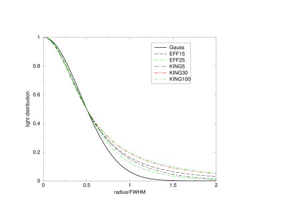
Figure 1: Fitted Gaussian FWHMs for input Gaussian profile convolved with WFPC2/WF3 F555W PSF, located on the central pixel. The diagonal solid line in the top panel represents a one-to-one relation, the other solid lines are the fifth-order polynomial fits to the data. Top: Output FWHM. Bottom: Output $-$ input FWHM.

Figure 2: Model light distributions.

2.2.2 Non-Gaussian input models

For a given FWHM, the less concentrated King/EFF model profiles have less light in the wings than more concentrated King/EFF profiles, while a comparable Gaussian profile has least flux in the wings. At radii smaller than the FWHM, non-Gaussian models appear somewhat more compact than a Gaussian profile. This is illustrated in Fig. 2.

In the first part of this study we adopt a fixed fitting radius of 5 pixels. We made this conscious choice for the fitting radius because for any realistic extragalactic SC observed with the HST at a decent S/N ratio, profile fits using Gaussian profiles are generally feasible. Larger fitting radii may be unproportionally affected by non-Gaussianity in the cluster profiles, low-S/N regions (i.e., fluctuations in the background noise), or neighbouring objects in crowded regions; much smaller fitting radii may not always be appropriate to employ Gaussian profile fits. To illustrate this, in Section 2.4, we will show that changing the fitting radius leads to systematic changes (and even numerical instabilities) of the ACs, and explain why this is the case.

Combining the choice of our 5-pixel fitting radius and the general behaviour of our input models, we expect to see the following trends:

• For clusters with input FWHM greater than 5 pixels, only the inner core will be fit. Due to the greater compactness of non-Gaussian models with respect to Gaussian profiles, for a given FWHM, we expect to systematically underestimate the sizes of large clusters.

• For clusters with FWHM smaller than 5 pixels, (i) the impact of PSF/diffusion kernel blurring of the cluster profile is more important, and (ii) the fit also includes the wings, which are more extended for non-Gaussian than for Gaussian profiles with identical FWHM. Therefore, we expect the sizes of small clusters to be overestimated.

• The 5-pixel boundary adopted was estimated from the size and shape of the cluster light profile alone. The application of PSF and diffusion kernel do not only change the size, but also the shape of the cluster profile. This causes unpredictable shifts in this empirical boundary. Nevertheless, we emphasise that the fit residuals are very small, as we will show below.

Since King models with large concentration indices and EFF models with small power-law index deviate most significantly from Gaussian profiles, we expect the largest deviations from a one-to-one relation between input and output FWHM for such models.

2.2.3 King profiles

For King profiles the results of this exercise are shown in Fig. 4. As expected, we find that for the less concentrated King-profile clusters, the relation between input and output FWHM deviates most from the relation for a Gaussian input model, i.e., from a strict one-to-one relation. The differences between King 5 and King 100 profiles reach $\sim 1$ pixel, with the King 5 results lying closer to the one-to-one relation.

Figure 3: Fitted Gaussian FWHM for input King profiles with different concentrations: $\ast$, $c$ = 5; $\blacksquare$, $c$ = 30; $\odot$, $c$ = 100. The diagonal solid line represents a one-to-one relation.

Figure 4: Fitted Gaussian FWHM for input EFF profiles with different power-law indices: $\ast$, $\gamma$ = 1.5; $\blacksquare$, $\gamma$ = 2.5. The diagnonal solid line represents a one-to-one relation.

2.2.4 EFF profiles

For young clusters in the LMC, which do not show any signs of tidal truncation, the best fit to the light distribution is a power law (Elson et al. 1987).

Fig. 4 shows the relation between input EFF-model FWHM and the FWHM of the Gaussian fit. The same systematic underestimate of large cluster sizes using Gaussian fits is observed as for the King models in the previous section, as expected. The differences between EFF 15 and EFF 25 profiles reach $\sim 1$ pixel, with the EFF 25 profiles lying closer to the one-to-one relation.

2.2.5 Fitting using the respective input profiles

To disentangle the effects of assuming a Gaussian profile (instead of the assumed input profile) on one hand and of the PSF/diffusion kernel on the other we ran a set of simulations using the input profile as fitting profile (instead of a Gaussian). The results presented in Fig. 5 indicate that the strong non-linearity seen in Figs. 4 and 4 originate from using the Gaussian fitting profile instead of the “correct” (input) profile. Using the input profile as fitting profile causes only a general offset (broadening of the light profile due to the PSF and the diffusion kernel). Unfortunately, the use of EFF/King profiles for light profile fitting is not implemented as standard even in some uptodate image reduction software packages, while a Gaussian is (to our best knowledge). Therefore, while sticking to the generally applicable Gaussian fitting profile we point at the origin of the non-linearities of our results.

Figure 5: Fitting standard artificial clusters with different input profiles, using the input profile shape as fitting profiles (instead of the Gaussian). The diagnonal solid line represents a one-to-one relation. Top: Different King profiles. Bottom: Different EFF profiles.

2.2.6 Presentation of the fit results

We fit the relation between the input FWHM of various profiles and the output FWHM of the Gaussian fits using a fifth-order polynomial function. One example table for the conversions that relate the input to the output FWHM, and vice versa, is presented in Appendix A, Table 4. The latter relation is most important to deduce the intrinsic size of a source from the measured size.

For the size-dependent aperture corrections (which will be determined in Sect. 3) two example tables are included: one table for aperture corrections to infinite aperture as a function of the intrinsic FWHM of the object (presented in Appendix B, Table 5), and one table for aperture corrections to infinite aperture as a function of the measured FWHM of the object (presented in Appendix C, Table 6).

In the following subsections, we will show the results for the two physically most interesting input models only, the King 30 and the EFF 15 models. These represent the average cluster light profiles of old Milky Way GCs (e.g., Binney & Tremaine 1998) and YSCs in the LMC (Elson et al. 1987), respectively. Although the realistic light profiles differ significantly from a Gaussian profile, Figs. 4 and 4 show that the fits to our conversion relations are very accurate. For input FWHM $>$ 0.5 pixel the deviations of the fits from the data are always smaller than 4 per cent, while for smaller FWHM it might be as large as 10 per cent. The conversion functions for the standard cluster and for the full set of input models are given in Table 4.

All data are also available in electronic form from our website, at
http://www.astro.physik.uni-goettingen.de/$\sim$galev/
panders/Sizes_AC/ . This public dataset does not only include the parameters of the fitted conversion functions, but also the averaged data used for the fitting to allow for customized fit functions, interpolations etc.

2.3 Effect of cluster brightness: Fits and fit errors

Thus far, we considered bright, noiseless artificial clusters of a given magnitude ($V=10$ mag), “observed” in a 1s exposure.

We performed a series of simulations, varying the cluster magnitudes from $V=8$ mag to $V=14$ mag. The results are shown in Figs. 7 and 7. For each magnitude and cluster profile, the results from 40 independent runs were averaged to reduce the scatter. The data from the individual runs, including the associated 1$\sigma$ uncertainties are compiled in Figs. 9 and 9 to show the amount of scatter.

Figure 6: Fitted Gaussian FWHM for input King 30 profiles of different cluster magnitudes. Top: Output $-$ input sizes, simulated data and fitted polynomials. Bottom: Comparison of fit functions, using the $V=10$ mag fit function as reference.

Figure 7: Fitted Gaussian FWHM for input EFF 15 profiles of different cluster magnitudes. Top: Output $-$ input sizes, simulated data and fitted polynomials. Bottom: Comparison of fit functions, using the $V=10$ mag fit function as reference.

Clearly, the conversion relations depend only weakly on the magnitude of the cluster. Deviations arise because the scatter in the relation increases with decreasing S/N ratio per pixel, as e.g. caused by decreasing cluster brightness and/or increasing cluster sizes. In addition, for clusters with sauch low S/N ratios per pixel, the readout noise might have some impact. See Sect. 2.5 for further details.

Figure 8: Comparison for $V=10$ mag King 30 (upper panel) and EFF 15 (lower panel) clusters. Horizontal lines indicate $\pm$ 0.2 pixels and $\pm$ 0.5 pixels. The solid curved lines indicate the $\pm$1$\sigma$ range of the scatter. Shown are the differences of the individual runs with respect to the average value.

Figure 9: Comparison for $V=14$ mag King 30 (upper panel) and EFF 15 (lower panel) clusters. Horizontal lines indicate $\pm$ 0.5 and $\pm$ 1.0 pixels. The solid curved lines indicate the $\pm$1$\sigma$ range of the scatter. Shown are the differences of the individual runs with respect to the average value.

When we compare the results from Figs. 7 and 7 to those of Figs. 9 and 9, we see that the scatter/deviations in the former figures for fainter clusters is fully consistent with the intrinsic scatter caused by the random nature of the algorithm used to generate the artificial clusters, even for averaged results. For bright clusters (represented by the $V=10$ mag cluster), the random scatter is on the order of $\pm 0.1$ pixel in the FWHM (for clusters larger than about 8 pixels FWHM up to $\pm 0.2$ pixel in the FWHM, and up to $\pm 1$ pixel for clusters larger than 11 pixels FWHM). This scatter increases with decreasing cluster brightness (up to $\pm 0.4-0.5$ pixels in the FWHM for a $V=14$ mag cluster smaller than about 7 pixels FWHM, and up to $\pm 3$ pixels in the FWHM for clusters larger than 7 pixels FWHM). The increasing scatter for large clusters is caused by the lower S/N ratio per pixel. The data are all presented in terms of the individual absolute values from the different runs to illustrate the scatter. The median value scatters significantly less.

In summary, for the average cluster, the conversion relations for bright clusters can be applied to clusters of all magnitudes: For fainter clusters and at larger radii (hence for cases with low S/N ratios per pixel) the cluster-to-cluster variations get larger, but scatter symmetrically around the average conversion relation.

2.4 Fitting radius variations

BAOlab has the advantage that the fitting radius can be adjusted easily. In fact, the choice of fitting radius has a major impact on the cluster sizes that one determines, as we will show in this section. We performed tests using fitting radii in the range from 3 to 15 pixels (larger and smaller fitting radii did not lead to any meaningful results owing to numerical problems related to the convergence of the size fitting). As one can see from Figs. 11 and 11, the larger the fitting radius one adopts, the larger the apparent cluster radius one measures, and the stronger the deviations from the input values become. In fact, increasing the fitting radius seems to result in continuously increasing recovered cluster radii. This is caused by the impact of (i) the intrinsic profile mismatch between King and EFF profiles, and (ii) the PSFs/diffusion kernels and their non-Gaussianity. The fitting radius dependencies of the results will be significantly lower if one were to fit the clusters with the correct cluster light profile, including the right PSF and diffusion kernel. However, since we wanted to keep our study as generally applicable as possible, we did not make use of the respective functions BAOlab provides in the standard settings. However, we refer the reader to Section 2.6, where we discuss this in more detail.

As shown by Carlson & Holtzman (2001), even fitting King profiles (which are thought to be more realistic, at least for old globular clusters) to observed cluster profiles is fitting radius dependent. They attribute this behaviour to inaccuracies of the PSFs at small radii. And indeed, their situation is different from ours, in the sense that in our case we expect the intrinsic differences of the input profiles and the fitted Gaussian to dominate the fitting behaviour, not inaccuracies of the PSFs, while for Carlson & Holtzman (2001) the profile mismatch, if any, is likely smaller.

A selection of fit residuals is included in Appendix D, in Figs. 35 and 35, as a function of fitting radius and input cluster radius. The area shown covers the inner $5\times 5$ pixels. For fitting radii $<5$ pixels, the solution tends to become computationally unstable, as shown in Fig. 11.

For small clusters, the residuals shown in Figs. 35 and 35 are almost independent of the fitting radius, because in all cases the cluster is much smaller than the fitting radius. However, the residuals are significantly non-negligible, clearly showing the intrinsic difference in shape between Gaussian and King/EFF profiles.

For large clusters (we show the results for clusters with FWHMs of 5.0 and 10.0 pixels, respectively), the residuals are relatively small for small fitting radii (e.g., fitting radii on the order of the input FWHM), where the fit is dominated by the inner parts of the clusters, which resemble Gaussian profiles. For fitting radii greater than the FWHM, the cluster wings are given too much weight, resulting in strong deviations in the inner cluster parts and large residuals (just as for “small” clusters, discussed above). The maximum residuals increase by a factor 3–5 for fitting radii from 5 to 15 pixels. However, fitting the inner cluster parts only seems to be more promising for 2 reasons: (i) the inner cluster region resembles a Gaussian profile more closely, and hence fitting with a Gaussian function is less problematic, and (ii) the S/N ratio per pixel is higher in the inner parts than in the wings.

In summary, one would like to have a fitting radius large enough to give stable results (larger than 3 pixels, cf. Figs. 11 and 11), but small enough to fit mainly the cluster core rather than the wings, to avoid serious problems with structures in the immediate environment of the cluster (e.g., variable background, crowding effects, etc.) and to produce (close to) negligible deviations from the input size. In addition, as shown in Figs. 11 and 11, the impact of changing the fitting radius is such systematic and significant, that a single, generic value for the fitting radius is needed. Otherwise, the entire analysis in this paper must be done for each individual data set.

We therefore recommend the use of a generic fitting radius of 5 pixels (which should be applicable to almost all realistic observations), and emphasise that all results given in this paper were thus obtained.

Figure 10: Conversion relations for a standard cluster, using different fitting radii (given in pixel units in the legend).

Figure 11: Conversion relations for a standard cluster, using different fitting radii (given in pixel units in the legend). Displayed are the offsets of these relations from the relation for a fitting radius of 5 pixels.

2.4.1 Origin of the strong fitting radius dependence of the results

The cause of the strong fitting radius dependence of our size conversion relations most likely also causes the non-linearity of the size conversion relations, i.e., the shape difference between the intrinsic cluster profile (EFF or King profiles) and the Gaussian used for the fitting.

To test this hypothesis we have performed a set of simulations similar to the ones in the previous section, except now the fit models are the same as the input models, and they were convolved internally with the appropriate PSF and the diffusion kernel. The results, shown in Fig. 12, partially support our hypothesis, even though for large fitting and cluster radii the behaviour is still non-linear, and differs systematically among the fitting radii.

We conclude that in order to get a one-to-one correlation between input and output FWHM the fitting radius must be at least larger than the cluster radius. In case the fitting radius equals the cluster radius, the deviations from a one-to-one correlation are typically of the order of -0.2/-0.3 pixel, as can be seen in Fig. 12. However, these deviations/non-linearities are intrinsically taken into account in our results.

Figure 12: Conversion relations for a standard cluster, using different fitting radii (given in pixel units in the legend) and taking the input light profile, PSF and diffusion kernel into account.

2.5 Impact of the sky background

In this section we assess the importance of the sky background. We model $V=10$ mag and $V=14$ mag clusters, each with background levels of 0, 1, 3, 5, 10, 20, 30, 50, and 100 ADU (“counts”) per pixel. We use 20 independent runs, and show the averaged results in Figs. 14 and 14, and the associated plots illustrating the actual scatter in Figs. 16 and 16 for the selected magnitudes, $V=10$ and $V=14$ mag, respectively.

Since sky noise and readout noise have the same characteristics, this Section combines both effects.

On average, the results seem to be robust with respect to (constant) changes in the sky background. There is only a slight tendency for faint clusters on a strong sky background to appear marginally smaller (see Fig. 14).

The impact of (Poissonian) shot noise from the cluster itself is negligible.

In order to allow for a rough estimate of the S/N ratios for the clusters and background levels discussed in this Section we provide the approximate count rates in the peak pixel of selected clusters in Table 2.

Table 2: Count rates [in ADU] in the peak pixel of selected clusters, to approximate S/N ratios for the background levels

cluster’s FWHM	King 30	EFF 15	King 30	EFF 15
$[$pixel$]$	$V=10$	$V=10$	$V=14$	$V=14$
1.0	6200	7600	150	180
2.0	3100	4100	80	100
5.0	900	1200	25	30
10.0	300	400	8	10

Figure 13: Conversion relations for a $V=10$ mag cluster, taking sky noise into account. As reference, the data for a standard cluster are taken. The straight lines are at $\pm$ 0.2 pixel.

Figure 14: Conversion relations for a $V=14$ mag cluster, taking sky noise into account. As reference, the data for a standard cluster are taken. The straight lines are at $\pm$ 0.5 pixel.

Figure 15: Scatter for $V=10$ mag EFF 15 clusters, with varying sky levels (“BG”, in ADU). As reference, the average data are taken. The straight lines are at $\pm$ 0.2 and $\pm$ 0.5 pixels. The solid curved lines indicate the $\pm$1$\sigma$ range of the scatter.

Figure 16: Scatter for $V=14$ mag EFF 15 clusters, with varying sky level (“BG”, in ADU). As reference, the average data are taken. The straight lines are at $\pm$ 0.5 and $\pm$ 1.0 pixels. The solid curved lines indicate the $\pm$1$\sigma$ range of the scatter.

2.6 Using the appropriate PSFs for fitting

For four HST/WFPC2 filters we checked to what extent the filter-dependent PSFs affect the cluster size determinations. BAOlab allows one to consider the appropriate PSF when fitting the cluster size by convolving the Gaussian model clusters with the PSF specified. Hence we created clusters with PSFs for the HST/WFPC2 $U,B,V,I$-band equivalent filters; while fitting the size of the cluster, BAOlab took the appropriate PSF into account. Here, we investigate the impact and possibilities of this approach.

The results are presented in Fig. 18. While the relations appear to be slightly noisier (despite the use of 40 independent runs), the differences between the different filters are well within the “normal” scatter of $\pm 0.2$ pixel.

Figure 17: Conversion relations for a standard cluster, using the appropriate PSFs for the fitting. The horizontal lines indicate $\pm$0.2 pixel.

Figure 18: Conversion relations for a standard cluster, using different filters for the ACS/WFC (chip 1).

2.7 Other dependences

We investigated the results for different WFPC2 filters and chips. Both variations lead to only minor differences in the results for the “standard” cluster. However, for completeness we give the results at our webpage.

We also checked the dependence of the results on the position of the artificial cluster on the chip, and on subpixel shifts. Both tests gave results within the “standard” random scatter of $\pm 0.2$ pixel.

In addition, we produced a number of PSFs assuming various spectral types for the standard cluster, ranging from O5 to M3. Again, all differences remain within the usual random scatter of $\pm 0.2$ pixel.

These “non-dependencies” are consistent with Carlson & Holtzman (2001), who found that different PSFs only have a minor impact.

2.8 Observing with ACS: chip, position, and filter dependence

Since both of the HST ACS/WFC chips (WFC1 and WFC2) are located well off the instrument’s optical axis, the PSFs suffer from severe geometrical distortions and the diffusion kernel is both wavelength and position dependent. Therefore, we carried out simulations with Tiny Tim PSFs for both WFC chips, for various positions on the chip, and – for the central positions of each camera – also using different filters (F435W, F555W, and F814W, roughly equivalent to Bessell-Johnson-Cousins $B,V$ and $I$). Again, 40 independent runs were used to obtain average values with reduced scatter.

The results for the different filters used with the ACS/WFC are shown in Fig. 18. The strongest differences are observed for the F814W filter, for which the sizes we determined are systematically larger, by $\sim 0.1-0.2$ pixels, than those obtained for the F555W filter. The reason is not quite clear, as both the PSF and the diffusion kernel appear less extended than the respective values for the F555W filter. In addition, Fig. 18 shows prominent discontinuities for the F814W filter around input FHWMs of 0.7 pixel. These peaks are statistically significant, and apparent in almost every single run.

The differences in the F435W filter are significantly smaller. In addition, when comparing the results for the F555W passband for the two WFC chips, we find only small differences. The deviations in the latter two cases are below or on the order of $\pm 0.05$ pixel.

Despite the distortion of the chips and the corresponding changes in the PSF with position across the chip, we find only a small impact on the derived sizes of the cluster position on the chips. For almost all clusters the deviations are well within $\pm 0.1$ pixel. Hence, for almost all purposes the central PSF (and the associated diffusion kernel) can be used.

2.9 Observing with NICMOS: filter-dependence

PSF construction for NICMOS using Tiny Tim is not straightforward, mainly because of the off-focus setting during early observations [i.e., before servicing mission 3B]. This caused strong temporal PSF dependences. The results discussed here are for two distinct observation dates. After inspection of a coarse grid of PSFs for different observation dates, we selected Tiny Tim PSFs for 1998 February 1 (as an example of a fairly blurred PSF) and “after 2002 September 29” (fully installed cryocooler phase, with only minor PSF blurring).

In both cases, a strong filter dependence is apparent, as can be seen in Fig. 19. For this reason, we give size conversions for all filters analysed (NICMOS equivalents to $J$, $H$ and $K$) and both epochs of observations at our webpage.

Figure 19: Conversion relations for a standard cluster (Upper panel: King 30 profile; Lower panel: EFF 15 profile), using different filters for NICMOS camera 2.

2.10 Further sources of uncertainties

Before assessing further possible sources of uncertainties we remind the reader that our study does NOT aim at working at the spatial resolution limit of HST (marginally resolved sources were already studied in Carlson & Holtzman 2001), but advice the users to apply our recipes only for clusters with an intrinsic FWHM greater than 0.5 pixel. Hence many of the tiny details and uncertainties inherent to PSF modelling (both theoretically as Tiny Tim and using observed PSFs) smear out, becoming irrelevant for our studies.

Drizzling and jitter might blur images slightly by broadening the PSF. However, as Carlson & Holtzman 2001 stated already (for an even more difficult situation, due to their smaller clusters, compared to ours) both effects have minor impact. The exact amount depends on the brightness of the source, the quality of the image reduction software to perform subpixel alignment, the number of exposures stacked, the length of these exposures etc..

For faint sources even at radii close to the peak the count numbers per pixel might reach values where Poisson statistics is non-negligible. However, this problem is intrinsic when dealing with faint sources. We have tried to quantify this effect in Figs. 9, 9, 16, and 16. For a further assessment and comparison with the widely-used DeltaMag method see Sect. 5.

To fully utilize the subsampling of the PSF, the use of a subsampled charge diffusion kernel/subsampled response function would be best, including its wavelength dependence. However, these are not available, and not likely to become available (see Tiny Tim FAQ page).

Other uncertainties, like breathing, desorption, scattering by dust, scratches or the electrode structure, the presence of ghost images etc. are complex and beyond any realistic measuring and modelling effort. However, most of these uncertainties are shared with observed PSFs.

3 Determining accurate photometry: Aperture corrections

3.1 Input parameters

We generate artificial clusters of different light profiles and sizes, $R_{\rm cl}$, using the BAOlab package and convolve them with the PSFs and diffusion kernels appropriate for the different cameras. We then determine ACs as a function of the FWHM of the source and the size of the aperture, $R_{\rm ap}$.

The aperture correction (AC_λ) is defined as:

$${\rm AC}_{\lambda} = -2.5\log\Bigl{(}F_{\lambda}(R_{{\rm ref}},R_{{\rm cl}})/F_{\lambda}(R_{{\rm ap}},R_{{\rm cl}})\Bigr{)}$$ (6)

$$= {\rm mag}_{\lambda}(R_{{\rm ref}},R_{{\rm cl}})-{\rm mag}_{\lambda}(R_{{\rm ap}},R_{{\rm cl}})\quad,$$ (7)

where $F_{\lambda}(R)$ is the flux within an aperture with radius $R$, and mag${}_{\lambda}(R)$ the corresponding magnitude, both for a given wavelength (filter) $\lambda$. The “ref(erence)” radius, $R_{\rm ref}$, is either infinity or another radius taken for reference, e.g., 0.5 arcsec (as recommended, e.g., by Holtzman et al. 1995). However, we will show that correcting to 0.5 arcsec, while appropriate for point sources, is insufficient for extended objects.

We consider three cluster light profiles in the remainder of this study:

• King 5: King profiles with $c=5$. This corresponds to the average concentration index observed for Galactic open clusters (e.g., Binney & Tremaine 1998); we emphasise, however, that because of the peculiar cluster profile and the large extent of the HST PSFs, the size and AC relations for King 5 profiles are more uncertain than for the other profiles;

• King 30: King profiles with $c=30$, corresponding to the average concentration index observed for Galactic globular clusters (e.g., Binney & Tremaine 1998);

• EFF 15: Elson, Fall & Freeman models with a power-law index of 1.5, matching the average observed profile of young populous LMC clusters (Elson et al. 1987).

Clusters with FWHMs between 0.1 and 15 pixels were considered, for each chip. For the clusters with small FWHMs, PSF photometry might be a more accurate solution. For this purpose the HSTphot package of Dolphin (2000) is available. However, since this package only works with very specific data formats, we cannot present a direct comparison of both methods here. Clusters larger than 15 pixels FWHM are very unlikely to occur, in particular since they must be very bright to have sufficiently high S/N ratios out to such large radii. For such clusters, additional effects become important, including background contamination and crowding.

The analysis was done for the WFPC2 PC and WF3 chips, for the ACS/WFC1 (WFC2 is equivalent) and for the NICMOS/NIC2 (pre and post-cryocooler) chips.

After generating and convolving the clusters with the appropriate PSF and diffusion kernel (where relevant), aperture photometry of the noiseless objects was done using different apertures. The ACs were determined with respect to the reference aperture. If not otherwise specified $R_{\rm ref}=50$ pixels is used. No model exhibits strong changes in the light profile for such large radii, hence $R_{\rm ref}=50$ pixels is sufficiently close to $R_{\rm ref}=\infty$ for our purposes.

3.2 The relation between aperture correction and input FWHM

First, we determine the relation between AC and input FWHM of the object.

The result is again fitted with a fifth-order polynomial function,

$${\rm AC}(x)=a+b*x+c*x^{2}+d*x^{3}+e*x^{4}+f*x^{5}\,,$$ (8)

where $x$ is the input FWHM of the object (in pixels), and $a$ through $f$ are the fitting coefficients.

An example is shown in Fig. 20. The bottom panel shows that the differences between the data and the fits of the form of Eq. (8) are smaller than 0.0025 mag. Hence, the fits are very accurate.

In Holtzman et al. (1995), the amount of missed light outside a 0.5 arcsec aperture is estimated to be $-0.1$ mag for point sources. Fig. 21 shows that the correction to a radius of 0.5 arcsec deviates by much more than $-0.1$ mag from the correction to an infinite aperture for extended objects. This confirms, again, the importance of correcting for the size of an object, and of including all of its flux.

Figure 20: Upper panel: Theoretical AC values (to infinite radius) for EFF 15 profiles with different FWHMs, and best fit results. The aperture sizes used are given. Lower panel: Deviations of data from fits.

As an example the fit results for the standard cluster are tabulated in Table 5. The full set of data is presented at our webpage.

Figure 21: Theoretical AC values for EFF 15 profiles with different FWHMs, and best fit results. The aperture size used is 3 pixels: $\Delta$ corrected to a 0.5 ″aperture; $+$ corrected to an infinite aperture; $\blacksquare$ shows the difference between the former two, hence the correction 0.5 ″$\rightarrow$ $\infty$.

3.3 The relation between aperture correction and measured FWHM

By combining the results from Sections 2 and 3.2, we can now determine the more immediately applicable AC values as a function of the measured FWHM.

An example of the fit results is shown in Fig. 22. The fit results for the standard cluster are tabulated in Table 6. The full data set is presented at our webpage.

The polynomial fits to the data using the measured FWHM are less satisfactory than the fits using the intrinsic sizes. The deviations are, depending on the cluster profile and the PSF used, on the order of $\pm 0.01-0.1$ mag, distributed fairly homogeneously over this range; see Fig. 22 for two extreme examples.

Figure 22: Upper panel: Theoretical AC values (to infinite radius) for EFF 15 profiles with different measured FWHMs, and best fit results. The aperture sizes used are given. Lower panel: Deviations of data from fits, covering the whole range of fit accuracies.

3.4 Sky oversubtraction

The most often used and most practical way to subtract the sky background from the cluster light is by defining a sky aperture around the cluster and subtracting the sky level. However, in most cases the sky annuli have to be chosen fairly close to the cluster to avoid confusion with nearby clusters or stars (i.e., crowding), gradients and strong variations in the sky background, among others. Because of the possibly large extent of the combination of the cluster and HST PSF, this “sky” subtraction likely also subtracts cluster light, in general. To obtain the actual cluster magnitude, this oversubtraction must be corrected for. We found as correction term (in magnitudes):

$$\Delta{\rm mag}_{1}=2.5\log\left(1-A\times F\right)\quad,$$ (9)

with area ratio

$$A=\frac{r^{2}_{1}}{r^{2}_{3}-r^{2}_{2}}\quad,$$ (10)

and flux ratio

$$F=\frac{10^{0.4{\rm AC}(r_{3},s)}-10^{0.4{\rm AC}(r_{2},s)}}{10^{0.4{\rm AC}(r_{1},s)}}\quad,$$ (11)

where $r_{1},r_{2}$ and $r_{3}$ are the sizes of the source annulus, and inner and outer sky annuli (in pixels), $s$ is the measured cluster FWHM (in pixels), and AC$(r_{i},s)$ are the aperture corrections (given as an example in Table 5 and the full data set at our webpage) for a given cluster size and given annuli. An example is given in Fig. 23. Using either AC_meas and $s_{\rm meas}$ or AC_intr and $s_{\rm intr}$ yields the same results.

Figure 23: Correction for sky oversubtraction as a function of input FWHM, following Eq. (9), for a 3-pixel source annulus, 5/8-pixel inner/outer sky annulus, and an EFF 15 profile.

3.5 Filter dependence

The same analysis as in Section 3.2 was done for all WFPC2 filters. Suchkov & Casertano (1997) found that for apertures of 3 or more pixels, the largest filter dependence (compared to F555W) of the ACs was 0.06/0.03 mag (in the F814W band, for the PC/WF3 chips, respectively). From 5 pixels onward and for the F439W band (the only other band apart from F555W and F814W considered in Suchkov & Casertano 1997), the differences are on the order of 0.01 mag. For the extreme case of a 3-pixel aperture, the differences between the F336W, F439W and F814W bands with respect to the F555W band are shown in Fig. 24. We clearly confirm the results of Suchkov & Casertano (1997). Only for the F814W band of the PC chip we get 0.08 mag, i.e., 0.02 mag larger than Suchkov & Casertano (1997), but most likely within the combined uncertainties of both studies.

Figure 24: Filter dependence of the AC for a 3-pixel aperture, in $UBVI$ for the WF3 (upper panel) and the PC (lower panel) chip of the WFPC2, and assuming an EFF 15 profile.

3.6 Subpixel shifts of clusters and the impact on the aperture corrections

Since observed clusters do not exhibit a smooth analytic profile but are modified by the pixel structure of the chip, subpixel shifts of the clusters and the accompanying redistribution of counts can change the photometry of the clusters and the aperture corrections. The changes are expected to be strongest for small apertures. In Fig. 25 we show the absolute differences of ACs for differently centered clusters (and the photometry annuli centered at the cluster). In Fig. 26 we show the relative differences of ACs for differently centered clusters (and the photometry annuli centered at the cluster). The figures show the expected behaviour of smaller apertures suffering from larger deviations. For 3 pixel annuli the differences caused by centering changes can be up to 0.25 mag, but for larger annuli even the maximum deviations are below 0.1 mag (corresponding to deviations of less than 20 per cent in almost all cases).

Figure 25: ACs for clusters with subpixel shifts relative to the [0;0] point, assuming a standard cluster with an EFF 15 profile. Shown are the absolute deviations between differently centered clusters with respect to the fit for the cluster at [0;0]. Top panel: AC 3 pixels $\rightarrow\infty$. Middle panel: AC 5 pixels $\rightarrow\infty$. Bottom panel: AC 8 pixels $\rightarrow\infty$.

Figure 26: ACs for clusters with subpixel shifts relative to the [0;0] point, assuming a standard cluster with an EFF 15 profile. Shown are the relative deviations between differently centered clusters with respect to the fit for the cluster at [0;0]. Top panel: AC 3 pixels $\rightarrow\infty$. Middle panel: AC 5 pixels $\rightarrow\infty$. Bottom panel: AC 8 pixels $\rightarrow\infty$.

The photometric centering is much less of an issue for our method, thanks to the fairly large apertures. The deviations are always below 0.04 mag, corresponding to less than 13 per cent in all cases. This is shown in Figs. 27 and 28.

Figure 27: ACs for clusters with annuli shifts relative to the [0;0] point, assuming a standard cluster with an EFF 15 profile. Shown are the absolute deviations between differently centered annuli with respect to the fit for the cluster at [0;0]. Top panel: AC 3 pixels $\rightarrow\infty$. Middle panel: AC 5 pixels $\rightarrow\infty$. Bottom panel: AC 8 pixels $\rightarrow\infty$.

Figure 28: ACs for clusters with annuli shifts relative to the [0;0] point, assuming a standard cluster with an EFF 15 profile. Shown are the relative deviations between differently centered annuli with respect to the fit for the cluster at [0;0]. Top panel: AC 3 pixels $\rightarrow\infty$. Middle panel: AC 5 pixels $\rightarrow\infty$. Bottom panel: AC 8 pixels $\rightarrow\infty$.

4 Cookbook for size-dependent aperture corrections

This subsection describes the most efficient use of the tables presented in this paper to apply to observations. We will use one object as an example.

• Fit a Gaussian profile to your source, using the appropriate parameters:

  • Use a fitting radius of 5 pixels (as shown in Section 2.4, the fitting radius has a significant impact on the size determination).

  • Use the co-added images also used for the photometry. We suggest the use of images roughly in the wavelength range between the $B$ and $I$ band, unless some of these filters have significantly lower S/N ratios than other available filters.

• Determine the flux-weighted mean of the sizes. This assumes a wavelength-independent size, and hence no mass segregation or similar effects. If there is good reason to expect such effects one should treat the photometry of each filter independently.

• If the size that is determined is smaller than one of the relevant PSF sizes (see Table 3) and larger than an apparently reasonable lower size cut-off (perhaps on the order of $0.5-1.0$ pixels; sources with even smaller radii will most likely be spurious detections), set the size to the PSF size, which can be found in Table 3 (these sources are most likely point sources).

• Choose the most relevant cluster profile; see Section 3.1 for help.

• Perform (circular) aperture photometry by choosing appropriate source and sky annuli.

• Calculate the aperture correction, using the annuli and measured size, and the polynomials from Table 6 or as obtained from our webpage.

• Calculate the oversubtracted cluster light, using Eq. 9, the annuli and measured size.

• Add the measured cluster magnitude, the calculated aperture correction and oversubtraction correction to obtain the cluster magnitude. Check that both corrections are negative; otherwise set to zero.

5 Comparison of our method with the widely used DeltaMag method

5.1 Size determination

Since many authors prefer other methods to determine sizes and aperture corrections, we compare our results with results from the most widely used method in this section.

The most commonly used measure of size is the magnitude difference in two concentric apertures (hereafter referred to as the “DeltaMag method”). A commonly used definition involves apertures of radii 0.5 and 3 pixels. A first obvious difficulty of using 0.5 pixel radii apertures is the centering, the distribution of the photons onto the relevant pixels and the accurate measurement of this effect. In addition, a Gaussian profile is usually assumed.

In the following, we will use our BAOlab cluster models to estimate the size determination accuracy for the DeltaMag method. We used our standard cluster settings and measured the magnitudes in apertures with radii of 0.5 and 3 pixels. For our three main models, the resulting magnitude differences as a function of input FWHM is shown in the top panel of Fig. 29. The impact of the centering is displayed in the middle and bottom panels of Fig. 29. Two types of centering have to be distinguished; (i) the centering (or exact positioning down to subpixel levels) of the cluster on the pixels of the CCD, and (ii) the photometric centering (the centering of the photometric annuli, or more generally the exact determination of the position of the cluster at subpixel levels). As shown in the middle and bottom panels of Fig. 29, the DeltaMag method is very sensitive to both kinds of centering problems.

We emphasize that the photometric centering is an integral part of BAOlab; hence is not a major problem for our method. In addition, the impact of incorrect centering is much more severe for a 0.5-pixel aperture compared to our standard aperture of 3-pixel radius. See Section 3.6 for the impact of subpixel shifts on the ACs for our method.

Figure 29: Top panel: $\Delta$mag between 0.5 and 3 pixels, for 3 different profiles. Middle panel: Comparison of $\Delta$mag for off-centered aperture annuli for the EFF 15 profile. Bottom panel: Comparison of $\Delta$mag for different centerings of clusters on a pixel, using an EFF 15 profile.

Another source of uncertainties intrinsic to the DeltaMag method results from the photometric uncertainty for each annulus. Assuming a photometric accuracy in $\Delta{\rm mag}\simeq\pm 0.1$ mag (which might even be too small for the 0.5 pixel annulus, because of centering issues), we determine how far off the size determination gets. The results are shown in Fig. 30 for two cluster light profiles. As a comparison we plot the accuracy limits for our method, determined by the stochastic effects during cluster formation (generation). In both cases the maximum deviations are calculated, and shown in Fig. 30. This result further strengthens the confidence we have in our method. The improvement in accuracy from the DeltaMag to our method is on the order of a factor 3–10.

The situation for faint clusters is not as unambiguous, as shown in Fig. 31. However, the improvement is still visible, but somehwat harder to quantify.

Figure 30: Scatter in the size determination from the DeltaMag method (assuming a photometric accuracy of $\pm 0.1$ mag), compared to the scatter introduced by our method for a standard cluster. Top panel: King 30 profile. Bottom panel: EFF 15 profile.

Figure 31: Scatter in the size determination from the DeltaMag method (assuming a photometric accuracy of $\pm 0.1$ mag), compared to the scatter introduced by our method for a $V=14$ mag cluster. Top panel: King 30 profile. Bottom panel: EFF 15 profile.

5.2 Aperture corrections

As we have shown in the previous section, our size determination method represents a significant improvement compared to the widely used DeltaMag method. While this is important in its own right, the accuracy of the AC calculations (and hence the determination of reliable absolute magnitudes for extended spherically symmetric sources) is of even greater importance.

While the size uncertainties correlate directly with the AC uncertainties, because of the non-linearity of the ACs we give the AC uncertainties for a number of cases in Fig. 32. The improvement of our method with respect to the DeltaMag method is clearly seen. Quantitavely, the mean improvement represents a factor of $\sim$ 6–9, covering a total range of 3–40. We emphasize that the uncertainties stated here for the DeltaMag method take into account only the uncertainty arising from a generic uncertainty in the magnitude determination of 0.1 mag. We take the AC relations determined in this paper, while there might be additional differences/uncertainties related to the DeltaMag as used in the papers cited, especially the mentioned centering problems.

Figure 32: Scatter in the AC calculation from the DeltaMag method (assuming a photometric accuracy of $\pm 0.1$ mag), compared to the scatter introduced by our method for a standard cluster. Top panels: 3 pixel radius apertures for an EFF 15 profile (left) and a King 30 profile (right). Bottom panels: Assuming an EFF 15 profile, and using 5 pixel (left) and 8 pixel (right) radius apertures.

6 Summary

We have presented an update to and significant improvement of the commonly used method of aperture photometry for HST imaging of extended circularly symmetric sources, including a reliable algorithm to determine accurate sizes of such objects.

Aperture photometry, by definition, underestimates the flux of any source if finite apertures are used. This is particularly relevant for HST imaging owing to the large extent of the PSFs, and the high spatial resolution, which makes small apertures possible and desirable to overcome crowding effects.

For this purpose, we investigated the possibilities to measure sizes of extended spherically symmetric objects accurately, and use this size information to obtain size-dependent ACs. This allows one to determine, in particular, masses of the objects based on integrated photometry more reliably, such as for extragalactic star clusters.

We modelled a large grid of artificial star clusters using a large range of input parameters, both intrinsic to the object (size, light profile, brightness, sky background) and observational (HST camera/chip, filter, position on the chip), using the BAOlab package of Larsen (1999). This package provides the user with good flexibility and realistic modelling of cluster light profile observations.

We first established the relationship between input size of a cluster (in terms of the FWHM of its light profile) and the measured size in terms of the FWHM of a Gaussian profile fitted to a given cluster. Bi-directional polynomial relations between these input and output FWHMs were established and collected in Appendix A and presented at our webpage.

In general, the differences between the results for different input parameters are only significant for (i) different input light profiles, (ii) different HST cameras, (iii) different fitting radii (maximum radius up to which the fit will be performed), (iv) (for NICMOS only) different observation epochs and filters, and (v) (for WFPC2 and ACS/WFC only) marginally significant for different filters and chips. Although we checked a large number of potentially important additional factors (such as, e.g., the exact position of an object on a certain chip, and the stellar spectrum used to create PSFs), we found the impact of those to be within the scatter introduced by the random effects inherent to cluster creation ($\sim\pm 0.2$ pixels).

Using the information thus obtained, we determined ACs for the same clusters that we determined sizes for. In Appendices B and C we present the results as a function of the intrinsic and the measured sizes of the clusters, respectively. The full data set is presented at our webpage.

As an example of the importance of using proper ACs for extended spherically symmetric sources, assume that we observe a cluster with an effective radius of 3 pc, located at a distance of 5 Mpc. Depending on the details of the observations and the data analysis, neglecting these size-dependent ACs may underestimate the brightness of the cluster by $0.3-1.3$ mag, corresponding to mass underestimates of $30-330$%.

In Section 4 we provide a cookbook for observers who aim to improve the accuracy of their aperture photometry of extended spherically symmetric objects.

Appendix A Parameters of cluster sizes fits

In this Appendix we present one example table containing the fit parameters of our cluster size studies (for our standard cluster).

The whole list of tables is provided at our webpage.

The fitting equations are

$${\rm size}(x)=a+b*x+c*x^{2}+d*x^{3}+e*x^{4}+f*x^{5}$$ (12)

and

$${\rm size}^{\prime}(y)=a^{\prime}+b^{\prime}*y+c^{\prime}*y^{2}+d^{\prime}*y^{3}+e^{\prime}*y^{4}+f^{\prime}*y^{5}$$ (13)

where $x$ and size${}^{\prime}(y)$ are the intrinsic FWHM in pixels, and size$(x)$ and $y$ the measured FWHM.

For reference, we also give the sizes of the PSFs as such, measured using the same procedure as for the clusters (Table 3).

Table 3: The sizes of the PSFs as such, measured using the same procedure as for the clusters. “Pre” and “Post” refer to either before or after the installation of the NICMOS cryocooler in the year 2002.

camera	epoch	filter	FWHM of PSF [pixel]
ACS WFC	$-$	$B$	2.26
ACS WFC	$-$	$V$	2.26
ACS WFC	$-$	$I$	2.19
NIC2	post	$J$	1.46
NIC2	post	$H$	1.67
NIC2	post	$K$	2.02
NIC2	pre	$J$	3.61
NIC2	pre	$H$	1.75
NIC2	pre	$K$	2.07
WFPC2 PC	$-$	$U$	1.70
WFPC2 PC	$-$	$B$	1.98
WFPC2 PC	$-$	$V$	2.12
WFPC2 PC	$-$	$I$	1.84
WFPC2 WF3	$-$	$U$	1.91
WFPC2 WF3	$-$	$B$	1.91
WFPC2 WF3	$-$	$V$	1.91
WFPC2 WF3	$-$	$I$	2.08

Table 4: Fit results of cluster sizes for a “standard” cluster. Upper panel: size$(x)$; Lower panel: size${}^{\prime}(y)$.

Profile	$a$	$b$	$c$	$d$	$e$	$f$
King5	1.63787	+1.03359	$-$0.00500374	$-$0.00943275	+0.000963603	$-$2.74858E-05
King30	2.04549	+1.52706	$-$0.297628	+0.0397823	$-$0.00242798	+5.51152E-05
King100	2.32858	+1.26613	$-$0.220773	+0.030224	$-$0.00193542	+4.67765E-05
Moffat15	1.91591	+1.18666	$-$0.144827	+0.0175979	$-$0.00104467	+2.43509E-05
Moffat25	1.73853	+0.873333	$-$0.00606163	$-$0.00245939	+0.000253589	$-$6.36749E-06
Profile	$a^{\prime}$	$b^{\prime}$	$c^{\prime}$	$d^{\prime}$	$e^{\prime}$	$f^{\prime}$
King5	$-$3.68916	+3.38959	$-$0.997741	+0.181195	$-$0.0137356	+0.000374692
King30	1.98751	$-$2.11849	+0.668887	$-$0.0351309	$-$0.00107904	+0.000109362
King100	3.72011	$-$4.16017	+1.49836	$-$0.189099	+0.0123212	$-$0.000330543
Moffat15	$-$0.243911	$-$0.476292	+0.387727	$-$0.0341423	+0.00154663	$-$3.25775E-05
Moffat25	$-$2.12227	+1.34245	$-$0.10647	+0.0244149	$-$0.00188937	+4.78649E-05

Appendix B Parameters of aperture correction fits: Intrinsic sizes

In this section we present one example table of the fit results for aperture corrections to infinite aperture as a function of intrinsic FWHM of the object. The full set of tables is provided at our webpage.

Table 5: Fit result of Eq. (8) to different apertures and models, for the correction to infinite aperture, as a function of the intrinsic size of a cluster. WF3 chip, F555W filter

King 5
Aperture (pixels)	$a$	$b$	$c$	$d$	$e$	$f$
2	$-$0.343217	$-$0.139042	$-$0.0866861	+0.0149747	$-$0.000997889	+2.38529e-05
3	$-$0.188471	+0.0272345	$-$0.0979988	+0.014184	$-$0.000869693	+1.97378e-05
4	$-$0.145765	+0.0814955	$-$0.0785946	+0.00961248	$-$0.000523544	+1.08528e-05
5	$-$0.119422	+0.0765121	$-$0.0512112	+0.00477206	$-$0.000192905	+2.83464e-06
6	$-$0.0969559	+0.0527979	$-$0.0274306	+0.00105827	+4.46585e-05	$-$2.68042e-06
7	$-$0.0760369	+0.0278805	$-$0.00969089	$-$0.00139504	+0.000188023	$-$5.77875e-06
8	$-$0.0598124	+0.00835219	+0.00180109	$-$0.00275704	+0.000256148	$-$7.03202e-06
9	$-$0.0471531	$-$0.00522251	+0.0086179	$-$0.00333541	+0.000271529	$-$7.01923e-06
10	$-$0.0389342	$-$0.0127713	+0.0117708	$-$0.00337635	+0.000254044	$-$6.2736e-06
11	$-$0.0322645	$-$0.0170747	+0.0127853	$-$0.00312398	+0.000220076	$-$5.19269e-06
12	$-$0.0277099	$-$0.0175305	+0.0118183	$-$0.00260648	+0.000171137	$-$3.80217e-06
13	$-$0.0237682	$-$0.0163978	+0.0101098	$-$0.00203923	+0.000122517	$-$2.48614e-06
14	$-$0.0205814	$-$0.014108	+0.00798676	$-$0.00146729	+7.67499e-05	$-$1.29518e-06
15	$-$0.018043	$-$0.0114669	+0.00590141	$-$0.00096043	+3.80676e-05	$-$3.20871e-07
King 30
Aperture (pixels)	$a$	$b$	$c$	$d$	$e$	$f$
2	$-$0.301938	$-$0.769798	+0.0909698	$-$0.00712295	+0.000302977	$-$5.25793e-06
3	$-$0.0947831	$-$0.518496	+0.0330069	+0.0001133	$-$0.000137099	+4.92056e-06
4	$-$0.0398307	$-$0.339737	$-$0.00407076	+0.00459379	$-$0.000407134	+1.11517e-05
5	$-$0.0261104	$-$0.222049	$-$0.0258731	+0.00714658	$-$0.000559794	+1.46668e-05
6	$-$0.0234392	$-$0.146405	$-$0.0378362	+0.00843162	$-$0.000632339	+1.62651e-05
7	$-$0.0228308	$-$0.0933415	$-$0.044637	+0.00904469	$-$0.000661937	+1.6827e-05
8	$-$0.0234847	$-$0.0565844	$-$0.0483172	+0.00929001	$-$0.000669692	+1.68934e-05
9	$-$0.0244382	$-$0.0293747	$-$0.049599	+0.00917832	$-$0.000652608	+1.63305e-05
10	$-$0.026445	$-$0.00885818	$-$0.0498729	+0.00896762	$-$0.000630663	+1.56775e-05
11	$-$0.027269	+0.00509821	$-$0.0488539	+0.00860091	$-$0.000599651	+1.48294e-05
12	$-$0.027888	+0.015614	$-$0.0473141	+0.00817894	$-$0.000565593	+1.39148e-05
13	$-$0.0274377	+0.0225115	$-$0.0452125	+0.00769632	$-$0.000527996	+1.29164e-05
14	$-$0.0266885	+0.0272389	$-$0.0427145	+0.00716421	$-$0.000487547	+1.18608e-05
15	$-$0.0253624	+0.029722	$-$0.040093	+0.00665291	$-$0.000450163	+1.09087e-05
EFF 15
Aperture (pixels)	$a$	$b$	$c$	$d$	$e$	$f$
2	$-$0.38549	$-$0.493638	+0.029603	$-$0.00100761	+6.40292e-06	+3.891e-07
3	$-$0.186551	$-$0.303161	$-$0.000318413	+0.00170018	$-$0.00012377	+2.93347e-06
4	$-$0.124193	$-$0.194666	$-$0.00875745	+0.00181114	$-$0.000104326	+2.17472e-06
5	$-$0.095772	$-$0.138253	$-$0.00840869	+0.00121683	$-$5.80395e-05	+1.04099e-06
6	$-$0.0785291	$-$0.107328	$-$0.00636706	+0.000716535	$-$2.66562e-05	+3.58918e-07
7	$-$0.0649638	$-$0.0867692	$-$0.00459549	+0.000402047	$-$9.93606e-06	+4.03718e-08
8	$-$0.0551751	$-$0.0722107	$-$0.00363422	+0.000284659	$-$7.07593e-06	+5.88729e-08
9	$-$0.0472316	$-$0.0608484	$-$0.00285465	+0.000197532	$-$4.52905e-06	+4.33668e-08
10	$-$0.0416458	$-$0.0518473	$-$0.00233845	+0.000147243	$-$3.39475e-06	+4.377e-08
11	$-$0.0371055	$-$0.0450427	$-$0.00174656	+7.82894e-05	$-$1.06734e-07	$-$2.52376e-08
12	$-$0.0330528	$-$0.0393012	$-$0.00141595	+5.6084e-05	+3.39864e-08	$-$1.56468e-08
13	$-$0.0288803	$-$0.035054	$-$0.000954172	+4.38475e-06	+2.75389e-06	$-$7.76727e-08
14	$-$0.0254902	$-$0.0307371	$-$0.000810798	$-$2.95168e-06	+2.8147e-06	$-$7.84767e-08
15	$-$0.0225039	$-$0.0270641	$-$0.000851373	+3.39294e-05	$-$9.68836e-07	+3.23473e-08

Appendix C Parameters of aperture correction fits: Measured sizes

In this section we present one example table of the fit results for aperture corrections to infinite aperture as a function of measured FWHM of the object. The full set of tables is provided at our webpage.

Table 6: Fit result of Eq. (8) to different apertures and models, for the correction to infinite aperture, as a function of the measured size of a cluster. WF3 chip, F555W filter

King 5
Aperture (pixels)	$a$	$b$	$c$	$d$	$e$	$f$
2	$-$0.678284	+0.489979	$-$0.218123	+0.0224476	$-$0.000971317	+1.51631E-05
3	$-$0.520845	+0.363595	$-$0.105187	+0.00161789	+0.000607791	$-$2.84509E-05
4	$-$0.203761	+0.00785934	+0.0525285	$-$0.0229136	+0.00230346	$-$7.24802E-05
5	0.0834688	$-$0.289561	+0.16345	$-$0.0380944	+0.00324296	$-$9.4625E-05
6	0.264027	$-$0.45638	+0.21616	$-$0.0436021	+0.00347388	$-$9.75032E-05
7	0.347541	$-$0.512145	+0.224791	$-$0.042163	+0.00321398	$-$8.7418E-05
8	0.362666	$-$0.497524	+0.208122	$-$0.0371469	+0.00272412	$-$7.17118E-05
9	0.333532	$-$0.439403	+0.176846	$-$0.0302172	+0.002123	$-$5.36127E-05
10	0.278828	$-$0.360897	+0.140408	$-$0.0229588	+0.0015276	$-$3.62966E-05
11	0.219309	$-$0.280452	+0.104876	$-$0.016226	+0.0009939	$-$2.11677E-05
12	0.154239	$-$0.198197	+0.0703799	$-$0.00998871	+0.000515741	$-$7.96413E-06
13	0.09792	$-$0.127794	+0.0415962	$-$0.00494001	+0.000140016	+2.12392E-06
14	0.051061	$-$0.0699366	+0.0185494	$-$0.00102533	$-$0.000140831	+9.38271E-06
15	0.0128557	$-$0.0234692	+0.000516643	+0.00194263	$-$0.000345926	+1.44674E-05
King 30
Aperture (pixels)	$a$	$b$	$c$	$d$	$e$	$f$
2	$-$1.48486	+1.72034	$-$0.781068	+0.116102	$-$0.00764245	+0.000188649
3	$-$1.99789	+2.20123	$-$0.868263	+0.126263	$-$0.00834	+0.000208911
4	$-$2.28948	+2.39106	$-$0.882108	+0.127079	$-$0.00843495	+0.000213594
5	$-$2.38265	+2.40546	$-$0.856241	+0.122881	$-$0.00819103	+0.00020892
6	$-$2.33809	+2.30984	$-$0.804295	+0.114912	$-$0.00765726	+0.000195477
7	$-$2.21033	+2.14933	$-$0.735909	+0.104439	$-$0.00692683	+0.000176048
8	$-$2.05979	+1.97861	$-$0.66855	+0.094201	$-$0.00620879	+0.000156785
9	$-$1.87339	+1.77785	$-$0.592421	+0.0824943	$-$0.0053717	+0.000133903
10	$-$1.70006	+1.59413	$-$0.524157	+0.0720706	$-$0.00462978	+0.000113704
11	$-$1.52497	+1.41483	$-$0.459317	+0.0622562	$-$0.00393567	+9.49368E-05
12	$-$1.36003	+1.24787	$-$0.399612	+0.0532495	$-$0.00329971	+7.77564E-05
13	$-$1.20427	+1.09316	$-$0.344983	+0.045026	$-$0.00271828	+6.19967E-05
14	$-$1.05245	+0.943919	$-$0.292809	+0.0372087	$-$0.00216874	+4.72173E-05
15	$-$0.929427	+0.825577	$-$0.252428	+0.0313432	$-$0.0017691	+3.67891E-05
EFF 15
Aperture (pixels)	$a$	$b$	$c$	$d$	$e$	$f$
2	$-$0.197547	+0.235124	$-$0.23533	+0.0334999	$-$0.00203347	+4.6805E-05
3	$-$0.284494	+0.347447	$-$0.202682	+0.0250798	$-$0.00135464	+2.79765E-05
4	$-$0.230654	+0.252511	$-$0.1295	+0.0130301	$-$0.000526366	+6.94963E-06
5	$-$0.145742	+0.143849	$-$0.0735813	+0.00512575	$-$4.44828E-05	$-$4.05185E-06
6	$-$0.0890236	+0.0785805	$-$0.0432653	+0.00151459	+0.000134323	$-$7.2046E-06
7	$-$0.0545739	+0.0428715	$-$0.0271714	+3.99231E-05	+0.000175742	$-$7.0894E-06
8	$-$0.0432793	+0.0326118	$-$0.0218415	+5.10128E-05	+0.000126706	$-$4.88752E-06
9	$-$0.0338311	+0.0243649	$-$0.017595	+2.71394E-05	+9.56854E-05	$-$3.52748E-06
10	$-$0.0269923	+0.0178575	$-$0.0141916	$-$3.10281E-05	+7.74326E-05	$-$2.70764E-06
11	$-$0.0211795	+0.0122217	$-$0.0112887	$-$0.000120992	+6.82416E-05	$-$2.26488E-06
12	$-$0.0190346	+0.0108055	$-$0.0101086	$-$3.68288E-06	+4.75348E-05	$-$1.56234E-06
13	$-$0.0130122	+0.00629541	$-$0.00799982	$-$9.31764E-05	+4.48676E-05	$-$1.39505E-06
14	$-$0.00965565	+0.00363862	$-$0.00636775	$-$0.000176703	+4.53483E-05	$-$1.37381E-06
15	$-$0.0140032	+0.0092721	$-$0.00803789	+0.000274421	+5.21679E-06	$-$1.87418E-07

Appendix D Illustrative figures

For illustration purposes, we present a comparative plot of the different light profiles (Fig. 33).

In Figs. 35 and 35 we present the fitting residuals for a number of differently sized clusters and a range of fitting radii.

In Fig. 36 we show the differences of WFPC2 PSFs across one chip, using the WF3 chip and the F555W filter.

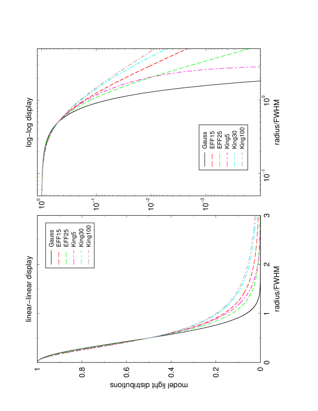
Figure 33: Various model light distributions. Left: Double-linear display. Right: Double-log display.

Figure 34: Light profile residuals of King 30 clusters. Rows (from top to bottom): FWHM = 0.5, 5.0 and 10.0 pixels. Columns (from left to right): fitting radius = 5, 9, 15 pixels. Color scale is linear, with very dark/bright regions having the largest deviations. Gray-scales are identical within a row.

Figure 35: Light profile residuals of EFF 15 clusters. Rows (from top to bottom): FWHM = 0.5, 5.0 and 10.0 pixels. Columns (from left to right): fitting radius = 5, 9, 15 pixels. Color scale is linear, with very dark/bright regions having the largest deviations. Gray-scales are identical within a row.

Figure 36: PSFs for the WF3 chip and the F555W filter, plotted using logarithmic color coding. The position in the image corresponds to the respective position on the chip. The PSFs were created subsampled by a factor of 10, the displays show $200\times 130$ pixels per PSF, corresponding to $2\times 1.3$ arcsec for an observation.