Hubble Space Telescope Observations of SV Cam: I. The Importance of Unresolved Starspot Distributions in Lightcurve Fitting

Abstract

We have used maximum entropy eclipse mapping to recover images of the visual surface brightness distribution of the primary component of the RS CVn eclipsing binary SV Cam, using high-precision photometry data obtained during three primary eclipses with STIS aboard the Hubble Space Telescope. These were augmented by contemporaneous ground-based photometry secured around the rest of the orbit. The goal of these observations was to determine the filling factor and size distribution of starspots too small to be resolved by Doppler imaging. The information content of the final image and the fit to the data were optimised with respect to various system parameters using the $\chi^{2}$ landscape method, using an eclipse mapping code that solves for large-scale spot coverage. It is only with the unprecedented photometric precision of the HST data (0.00015 mag) that it is possible to see strong discontinuities at the four contact points in the residuals of the fit to the lightcurve. These features can only be removed from the residual lightcurve by the reduction of the photospheric temperature, to synthesise high unresolvable spot coverage, and the inclusion of a polar spot. We show that this spottedness of the stellar surface can have a significant impact on the determination of the stellar binary parameters and the fit to the lightcurve by reducing the secondary radius from 0.794$\pm$0.009 R_⊙ to 0.727$\pm$0.009 R_⊙. This new technique can also be applied to other binary systems with high precision spectrophotometric observations.

1 Introduction

Star-spots and other forms of magnetic activity are prevalent on rapidly rotating stars with temperatures low enough to have outer convective zones. The dynamo activity in these rapidly rotating cool stars leads to the suppression of convection over large areas of the stellar photosphere. These giant starspots can modulate the light of such active stars as they rotate by up to tens of percent. In general, stars that exhibit this type of activity are solar-type stars with rotational periods of less than one day. This rapid rotation is seen in half the G and K dwarfs in open clusters younger than 100 Myr, and may also persist into middle age through tidal locking in a close binary systems such as RS CVns.

Doppler imaging is a powerful tool for determining where spots congregate on the stellar surface, but it is less successful at determining how much overall spot activity is present. Other methods such as TiO-band monitoring studies (O’Neal et al., 1998) indicate that between 30-50% of the stellar surface is spotted compared to 10-15% from Doppler imaging (Jeffers et al., 2002). The discrepancy in these methods can be accounted for if the stellar surface is heavily covered by spots that are too small to be resolved through Doppler imaging. To try to resolve this we have used the photometric capabilities of the HST (signal-to-noise $\simeq$ 5000) to eclipse-map the inner face of the F9V primary of the eclipsing binary SV Cam. Using these observations, Jeffers et al. (2005) found that the surface flux in the low-latitude region to be approximately 30% lower than the best fitting phoenix model atmosphere. A possible cause of this flux deficit is that the primary star’s surface is peppered with unresolvable spots. They also found that when the 30% spottedness is extended to the entire stellar surface there still remains a flux deficit, which could be explained by the presence of a large polar cap.

In this paper we use the Maximum Entropy eclipse-mapping code DoTS (Collier Cameron 1997; Collier Cameron & Hilditch 1997) to firstly solve for the system parameters of the lightcurve, and then reconstruct the surface brightness distribution of SV Cam’s primary star. We also show how a synthetic polar cap and the star being peppered with spots below the resolution limits of eclipse mapping are essential parameters for obtaining a good lightcurve fit.

Visit	Obs. Date	Frame No	UT Start	UT End	Julian Date (+ 52210)	Exposure Time (s)	Phase Range
1	01 Nov 01	1-48	21:04:33	21:47:44	4.879394-4.908758	30	0.901-0.950
		49-107	22:24:18	23:17:41	4.909383-4.971851	30	0.952-1.058
		108-165	00:00:23	00:51:58	5.001505-5.037328	30	1.107-1.168
2	03 Nov 01	166-213	14:43:36	15:26:47	6.614915-6.644280	30	0.828-0.877
		214-272	16:02:23	16:55:46	6.669628-6.706701	30	0.920-0.983
		273-330	17:38:27	18:30:02	6.736343-6.772167	30	1.033-1.093
3	05 Nov 01	331-378	14:43:36	15:26:47	8.416575-8.446561	30	0.865-0.916
		379-437	16:02:23	16:55:46	8.470752-8.507825	30	0.957-1.019
		438-495	17:38:27	18:30:02	8.537468-8.573291	30	1.069-1.13

Table 1: Journal of observations for SV Cam using the Space Telescope Imaging Spectrograph on board the Hubble Space Telescope

2 Observations

SV Cam (F9V + K4V, P=0.59d, vsini=102 km s^-1, $i$=90^∘) is a totally eclipsing, short-period binary system originally identified by Guthnick (1929). Contemporaneous HST and ground based observations were obtained to eclipse map SV Cam. The ground based photometric observations were obtained to complete the light curve outside primary eclipse making it possible to determine any global asymmetry in the lightcurve due to the presence of any uneclipsed spots.

2.1 HST Observations

We observed three primary eclipses of SV Cam during three HST visits at intervals of 2 days between 2001 November 1 to 5. A total of 9 spacecraft orbits were devoted to the observations. The G430L grating of Space Telescope Imaging Spectrograph (STIS) was used to disperse starlight over 2048 CCD elements. The observations are summarised in Table 1 and the lightcurve for each visit is shown in Fig. 1.

The observations cover a wavelength range from 2900 Å   to 5700 Å, with an exposure time of 30 s and a cadence of 40 s. The exposure time was chosen as a trade-off between maximising signal-to-noise per exposure and minimising the time interval between observations. The total count over the entire detector is 9.4$\times$10⁷ electrons per exposure, with the photometric precision calculated to be 0.00015 magnitudes (S:N = 5000). The main source of systematic error, due to the subtle motion of the satellite, was removed by cross-correlating each frame with respect to a template spectrum, and then adding or subtracting a scaled number of counts. After correcting for this ‘jitter’ the RMS scatter was consistent with the error expected from photon noise.

Figure 1: The comprising sections of the primary eclipse from each of the 3 HST visits, with an off-set of 5$\times$10^-11 ergs/s/cm² for clarity.

2.2 Ground Based Photometry

The ground based photometric observations were obtained with the 0.93-m James Gregory Telescope (JGT) at the University of St Andrews, using a Wright Instruments CCD camera mounted at the Cassegrain focus. The observations were made with a narrow-band filter whose 85 Å (FWHM) bandpass is centred at 5300 Å, close to the V band. Using an exposure time of 60 s we obtained a photometric precision of $\pm 0.006$ mag in good photometric conditions. The overhead for the chip readout between 60 s observations is typically 15 s, giving an overall sampling interval of 75 s. Observations were made over a two week period centred at the time of the HST observations. The weather permitted the observation of four full primary eclipses and three full secondary eclipses over this period.

3 Data Processing

3.1 Data Reduction

Reduction of the HST data comprised calibrating the two dimensional CCD images and extracting one dimensional spectra using the standard STIS data reduction pipeline. A detailed description of this procedure is contained in the STIS handbook. This pipeline routine produces bias and dark subtracted, flat-fielded wavelength calibrated images. The auto-wavecal was disabled for these images, but instead two ‘Guest Observer’ wavecals were taken per orbit. Cosmic rays were removed using an algorithm that identifies and rejects cosmic rays and other non repeatable defects by comparing successive frames.

The ground-based photometric data were reduced using jgtphot, a software package developed for use with the James Gregory Telescope at St Andrews (Bell et al., 1993). The resulting light curves are calculated as differential magnitude values with respect to the marked comparison and check stars.

3.2 Time Correction of HST data set

As the time of the extracted one-dimensional spectra that is output from the standard STIS data reduction pipeline (calstis) is in UT, it is necessary to apply a further time correction to this value. The heliocentric correction due to the motion of the Earth around the Sun, and due to the orbital motion of the satellite was determined through use of the ‘odelaytime’ routine. To convert UT into atomic time 32 leap seconds were added, and to convert atomic time into terrestrial time 32.184 seconds were added, resulting in the correct terrestrial time value. Absolute precision in HST time is required as it is necessary to have the primary eclipse of the HST and of the ground-based observations exactly aligned.

3.3 Interpolation of Data Sets

In order to analyse the absolute spectrophotometry from STIS together with the ground-based differential photometry, it was necessary to place the magnitudes derived from the two instruments on a common magnitude scale. We constructed a synthetic filter, V_hst, with a bandpass and effective wavelength matching those of the filter used for the JGT observations, (bandpass of 80Å and effective wavelength 5300Å) and applied it to the HST observations. Similarly we constructed a digital version of the Johnson B filter, B_hst.

At the time of each JGT flux measurement during primary eclipse we interpolated the V_hst magnitude and the ($B_{hst}-V_{hst}$) colour index from the two nearest points bracketing the same phase. The colour equation relating the two magnitude systems was then derived by a linear least-squares fit to the plot of $\delta V_{jgt}-V_{hst}$ versus ($B_{hst}-V_{hst}$), as shown in Fig. 2. This yielded the colour equation

$$\delta V_{jgt}-V_{hst}=\alpha(B_{hst}-V_{hst})+\beta,$$ (1)

where the coefficient of the colour term $\alpha=-0.0725392\pm 0.05836$ and the zero-point $\beta=-8.69367\pm 0.03318$ magnitudes.

Using this linear calibration, all of the V_hst magnitudes were converted to the JGT system. This procedure takes account of the zero point off-set, the effect of the V_hst and the JGT observations having slightly different effective wavelengths, and the different spectral responses of the two filter sets and the two CCDs. The interpolated HST data set is shown in Fig. 2 along with the JGT data.

Figure 2: Interpolated HST data (primary eclipse) set plotted with JGT data set (secondary eclipse).

Ref.	Tpri	Tsec	Rpri		Rsec		i		q		S / P	Spectral Type
This work	6038(58)	4804(143)	1.	238(6)	0.	794(6)					P	F9V+K4V
(reduced Tphot + polar cap)	5935(38)	4808(143)	1.	235(7)	0.	727(6)					P	G0V+K4V
Lehmann et al. (2002)			1.	18(2)	0.	76(2)	90.	0	0.	642(5)	S	G0V+K6V
Rucinski et al. (2002)							90.	0	0.	641(7)	S	G2V(pri+sec)
Kjurkchieva et al. (2002)			1.	38(5)	0.	94(6)	80.	0	0.	593(11)	S	F5V+G8V
Albayrak et al. (2001)	6440	4467(34)	1.	38(2)	0.	87(2)	89.	6(9)	0.	56	P	F8V+K6V
Albayrak et al. (2001)	6200	4377(32)	1.	38(2)	0.	87(2)	89.	6(9)	0.	56(10)	P	F5V+K6V
Pojmanski (1998)			1.	25	0.	8	90.	0	0.	56(9)	S	F5V+K0V
Patkos & Hempelmann (1994)	5750	4500	1.	18(5)	0.	75(3)					P	G2/3V+K4/5
Rainger et al. (1991)							90.	0	0.	7	S	G2/3V+K4V
Zeilik et al. (1988)	5800	4300	1.	17(3)	0.	74(3)	89.	5(5)			P	G3V
Budding & Zeilik (1987)	5750	4500	1.	11(2)	0.	74(2)	90.	0(5)	0.	71	P	G3V+K4
Hilditch et al. (1979)	5800	4140	1.	224	0.	864	80.	0	0.	7	P	G3V+K4V

Table 2: Summary of observed stellar parameters for SV Cam from the literature where T_pri and T_sec are the primary and secondary photospheric temperatures (K), R_pri and R_sec are the primary and secondary radii (R_⊙), i is the binary system inclination (degrees), q is the secondary:primary mass ratio and S/P indicates spectroscopic or photometric observations.

4 Lightcurve Fitting

The combined HST and JGT lightcurve of SV Cam is fitted using the maximum entropy code dots. Included in dots is the ability to incorporate the surface geometry and radial velocity variations of tidally distorted close binary components (Collier Cameron, 1997) while solving for starspot coverage.

4.1 Eclipse Mapping

By using eclipse mapping it is possible to determine the detailed locations of low latitude spots on the stellar surface. If spots are present on the inner surface of the primary, that is occulted by the cooler secondary star, jagged discontinuities will be produced on the eclipse profile as the primary is occulted by the secondary. The timescales and amplitudes of these discontinuities will reflect the distribution of spot sizes on the inner surface of the primary.

4.1.1 Maximum Entropy

The maximum entropy method allows us to determine the simplest image of the primary’s surface (in terms of its information content as quantified by the Shannon-Jaynes image entropy), that can reproduce, at a specified goodness of fit, the perturbations to the primary eclipse.

For images where the mapping parameter $f_{i}$ is bolometric surface brightness and so can take any positive value, the entropy takes the form,

$$S=\sum_{i}(f_{i}-m_{i}-f_{i}\ln\frac{f_{i}}{m_{i}})$$ (2)

Here $m_{i}$ is the default value that a pixel will have when there are no other constraints imposed by the data. In this analysis a restricted form of the entropy is used as the filling-factor model has been adopted. This combines the entropy of the spot image $f_{i}$ and of the photospheric image $(1-f_{i})$:

$$S=\sum_{i}(-f_{i}\ln\frac{f_{i}}{m_{i}}-(1-fi)\ln\frac{(1-f_{i})}{(1-m_{i})}).$$ (3)

To construct the final image, the values for the spot and photospheric $f_{i}$ are iteratively adjusted to maximise;

$$Q=S-\lambda\chi^{2}$$ (4)

This is equivalent to maximising the entropy $S$ over the surface of a hyper-ellipsoid, of constant $\chi^{2}$, in image space. This is bounded by the constraint surface at some fixed value of $\chi^{2}$. The Lagrange multiplier, $\lambda$, is set so that the final solution lies on a surface with $\chi^{2}\simeq M$, $M$ being the number of measurements in the data set. By setting a Lagrangian multiplier, it is possible to determine the extrema (maximum) of the entropy, the image with the least information content, subject to the constraint of obtaining the best fit to the data. A more detailed explanation of this, and other methods, is discussed by Collier Cameron (2001).

It is important not to over fit $\chi^{2}$ during the reconstruction, as this can result in an ill-fitting photometric fit and artifacts on the final spot map. The number of iterations was set to 25, as through rigorous testing we found this to be the value where the final image did not contain any distortions due to ill fitting.

4.2 Geometric Parameters

The success of a surface image reconstruction depends largely on a correct determination of the geometric parameters of the binary system (Vincent et al 1993). Independent reconstructions for the starspot parameters and the geometric parameters of the system, are susceptible to the distortions in the lightcurve yielding the wrong system parameters or vice versa. If the system parameters are wrong, in general a satisfactory fit to the data is only obtained by increasing the amount of structure in the stellar surface brightness distribution, usually leading to a greater total spot area than is present when the correct geometric parameters are used.

The principal parameters that affect the shape of the light-curve of an unspotted star are the relative temperatures, the radii of the two stars and the system inclination. The relative surface brightnesses of the two components determine the relative depths of the primary and secondary eclipses. The radii of the two stars and the binary system inclination are related to each other by the orbital phases at which the four contact points occur (phase 0.906,0.977,1.023 and 1.093 respectively). These relations are further complicated by the presence of starspots which in general have the effect of altering the depth of the eclipses and making the contact points asymmetrical.

SV Cam has been the subject of numerous photometric and spectroscopic studies. Despite this, there still does not yet exist a established and reliable set of stellar parameters. The various published combinations of stellar parameters that can be found for SV Cam in the literature are summarised in Table  2. A discussion of the individual merits of each set of binary system parameters is beyond the scope of this paper. Given the wide range of geometric parameters available for SV Cam, it was necessary to determine a set of parameters that would give an optimal fit to our lightcurve.

In fitting the photometric lightcurve of SV Cam we use the mass ratio (q=0.641$\pm$0.007), semi-amplitude velocity (K₁=121.86$\pm$0.76, K₂=190.17$\pm$1.73) and systematic radial velocity (-9.31$\pm$0.78) of Rucinski et al. (2002) as their solution for SV Cam’s spectroscopic orbit is very well defined.

4.3 Temperature

Jeffers et al. (2005) determined the temperature of the separated primary and secondary components of SV Cam using phoenix (Allard et al., 2000) model atmosphere spectra. Model atmospheres, ranging in temperature from 5600 K to 6500 K in 100 K steps, were fitted to the spectrum of the primary and secondary stars using $\chi^{2}$ minimisation. The minimum $\chi^{2}$ value corresponds to a temperature of 6013$\pm$19 K and 4804$\pm$143 K for the primary and secondary stars respectively. The primary star was then isolated and fitted using the same method, where the minimum temperature is 6038$\pm$58 K. In this work we use the independently fitted primary temperature as the error estimate is more reliable.

4.4 Radii

The radii for the primary and secondary stars were determined using the robust grid search method. This method uses a grid of radii as input to DoTS ranging from 1.17 R_⊙ to 1.26 R_⊙ for the primary star, and 0.73 R_⊙ to 0.82 R_⊙ for the secondary star in 0.005 R_⊙ intervals. For each grid point a model with the specified set of geometric parameters was iterated 25 times to obtain the lowest value of the reduced $\chi^{2}$. The inclination was not included as it scales as (sin i)^-1, implying a negligible difference between inclinations of 90^∘ and 85^∘.

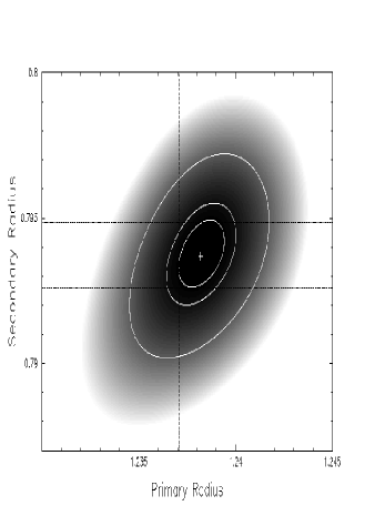
Figure 3: Contour plot of the $\chi^{2}$ landscape for the primary and secondary radii. From the centre of the plot, the first contour ellipse is the 1 parameter 1$\sigma$ confidence limit at 63.8%, the second contour ellipse is the 2 parameter 1$\sigma$ confidence limit at 63.8%, and the third contour ellipse is the 2 parameter 2.6$\sigma$ confidence limit at 99%.

The results for the $\chi^{2}$ minimisation are shown in Fig. 3 in the form of a contour plot. The minimum $\chi^{2}$ value occurs at 1.238 $\pm$ 0.007 R_⊙ and 0.794 $\pm$ 0.009 R_⊙ for the primary and secondary stars respectively. The best fitting stellar parameters for the combined JGT and HST data sets are summarised in Table  3.

4.5 Lightcurve Fit and Surface Brightness Image

The resulting Maximum Entropy fit to the lightcurve, using the stellar parameters as previously defined is shown in Fig. 4. The observed data minus computed lightcurve residuals are shown in Fig. 5 in enlarged form covering just the HST primary eclipse data. The stellar surface image that results from these fits is shown in Fig. 6.

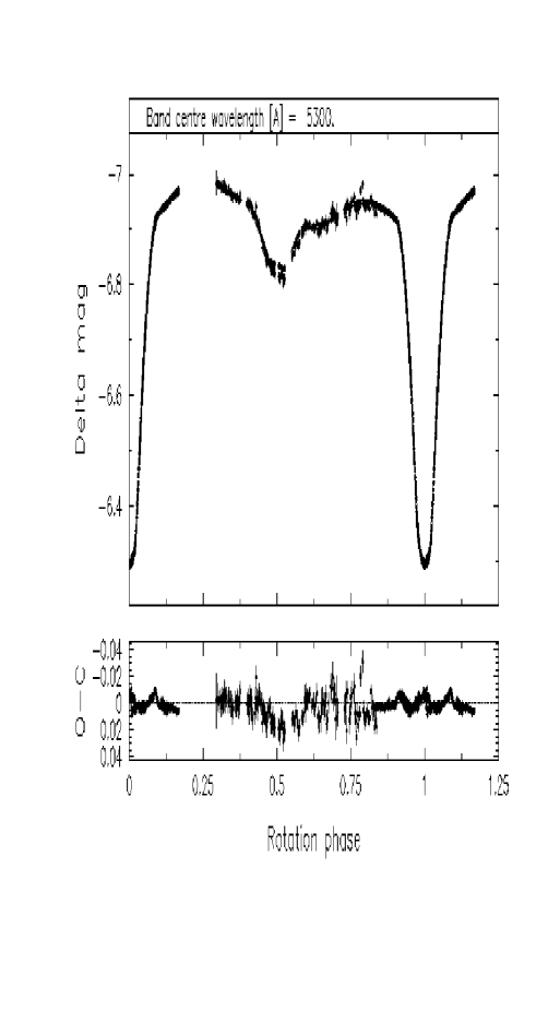
Figure 4: Combined HST and JGT lightcurves, with a Maximum Entropy fit.

Figure 5: Observed minus Computed residuals with no polar cap (HST data only). The four contact points are shown as vertical lines.

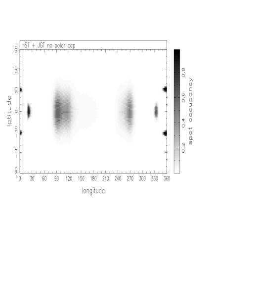
Figure 6: The final spot map of SV Cam (HST + JGT data). Note that phase runs in reverse to longitude. Spots reconstructed using $\chi^{2}$ and located at the quadrature points have been shown by Jeffers (2005) to be spurious. Note that phase runs in reverse to longitude.

The model lightcurve of the best fitting binary system parameters is shown in Fig. 4. When the modelled light-curve is subtracted from the observed data the residuals are symmetric about phase 1, and have two large discontinuities that occur at the first and fourth contact points either side of the primary eclipse (Fig. 5). Given the location of these discontinuities, an obvious explanation would be that the radius of either of the two stars has been incorrectly determined. However, the accuracy of our determination of the stellar parameters, as described in Section 4, can eliminate this possibility.

The surface brightness distribution (Fig. 6) shows two large spot features at the quadrature points similar to ’active longitudes’ that have been observed using photometry on other RS CVns (e.g. Olah et al. (1991), Lanza et al. (2001) and Lanza et al. (2002)). These spots are reconstructed at the equator as there is no eclipse information to determine the latitude. The spot at 100^∘ is stronger as that quadrature of the star has a higher spot coverage, which is also evident in the lower light level of the photometric lightcurve at phase $\approx$0.75. The spots reconstructed at 25^∘, 335^∘, and 360^∘ result from spots on the primary star that have been occulted by the secondary star during primary eclipse. The symmetry is due to the inability of DoTS to determine the hemisphere of the spot feature.

5 Unresolvable Spot Coverage

Parameter	sol. 1	sol. 2
Ephemeris	52214.34475 (MJD)
Tpri	6038 $\pm$58 K	5935 $\pm$38 K
Tsec	4804 $\pm$143 K	4804 $\pm$143 K
Rpri	1.238 $\pm$0.006 R⊙	1.235 $\pm$0.007 R⊙
Rsec	0.794 $\pm$0.006 R⊙	0.727 $\pm$0.006 R⊙
Polar Cap		46.7o

Table 3: Geometric binary system parameters computed for SV Cam. For solution 1, the primary and secondary temperatures are taken from Jeffers et al. (2005), while solution 2 shows the radii and polar cap size solved using a reduced photospheric temperature to synthesise the star being peppered with small spots.

5.1 Reduced Photospheric Temperature

Jeffers (2005) tested the limitations of surface brightness images from photometric data by modelling many sub-resolution spots on an immaculate SV Cam. Surface brightness distributions reconstructed from these synthetic lightcurves show distinctive spots at the quadrature points. The presence of similar spot features in Fig. 6 could indicate that the surface of SV Cam is peppered with many spots that are below the resolution capabilities of the eclipse mapping technique. This would then be consistent with the results of TiO band monitoring studies (O’Neal et al., 1998) which show that between 30% and 50% of a star’s surface may be spotted.

Further evidence for the peppering of the SV Cam’s primary star by small starspots is shown by Jeffers et al. (2005). As previously described in section 4, they determined the temperatures of the two stars using best-fitting phoenix model atmospheres. It was also found that the primary’s surface flux is approx 28% lower than predicted by a phoenix model atmosphere at the best fitting effective temperature. Even taking into account the spot distributions as shown in Fig. 6, this flux deficit can only be accounted for if the primary star’s surface is peppered with unresolved spots. As these spots are not resolvable using the eclipse-mapping technique they can lead to a under estimation of the star’s photospheric temperature and will have the effect of decreasing the flux deficit during the eclipse at all wavelengths.

To determine the reduced photospheric temperature, resulting from the presence of many unresolvable spots, we extend the work of Jeffers (2005). An extrapolated solar spot size distribution is applied to an immaculate SV Cam, for 1.8%, 6.1%, 18%, 48% and 100% area filling factors of spots, with T_ph=6038 K, and T_sp=4538 K. Each of these spot distributions is modelled as a photometric lightcurve, and is then used as input to the Maximum Entropy eclipse mapping code. To obtain a satisfactory fit to the lightcurve it was necessary to reduce the photospheric temperature to values as shown in Fig. 7. A quadratic fit to these points gives a temperature for 28% spottedness of 5935 K which is the average temperature over hotter and unresolvable cooler temperature regions.

Figure 7: The decrease of primary star’s photospheric temperature as a function of percentage of spot coverage on its surface.

5.2 Polar Spot

The work of Jeffers et al. (2005) also showed that in addition to the 28% spot coverage in the eclipsed region of the primary star, there is an additional 12.5% flux deficit in non-eclipsed regions of the star. The additional flux deficit can only be explained by the presence of a polar cap which would have the effect of increasing the depth of the primary eclipse, and would lead to an incorrect lightcurve solution.

We include a polar cap in our lightcurve solution by extending the 2-dimensional grid search described in section 4 to a 3-dimensional grid search including the polar spot size from 35^∘ to 50^∘. The polar spot is assumed to be at 4500 K, circular, centred at the pole, and is in addition to the reduced photospheric temperature as described above. For each polar spot size the minimum primary and secondary radii are determined using a $\chi^{2}$ contour map. These minimum $\chi^{2}$ values are plotted as a function of polar spot size in Fig. 8. The best fitting polar cap size, 46.7^∘ was determined from the minimum of a quadratic function fitted to these points. This value is in good agreement with the independently determined value of 42$\pm$6^∘ by Jeffers et al. (2005).

Figure 8: Quadratic fit to the variation of $\chi^{2}$ as a function of polar spot size.

The grid search of radii is then repeated using a fixed value for the polar spot size. The results for the $\chi^{2}$ minimisation are summarised in Table 3 and are shown as a contour map in Fig. 9.

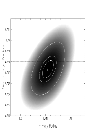
Figure 9: Contour plot of the $\chi^{2}$ landscape for the primary and secondary radii with a 46.69^∘ polar spot. From the centre of the plot, the first contour ellipse is the 1 parameter 1$\sigma$ confidence limit at 63.8%, the second contour ellipse is the 2 parameter 1$\sigma$ confidence limit at 63.8%, and the third contour ellipse is the 2 parameter 2.6$\sigma$ confidence limit at 99%.

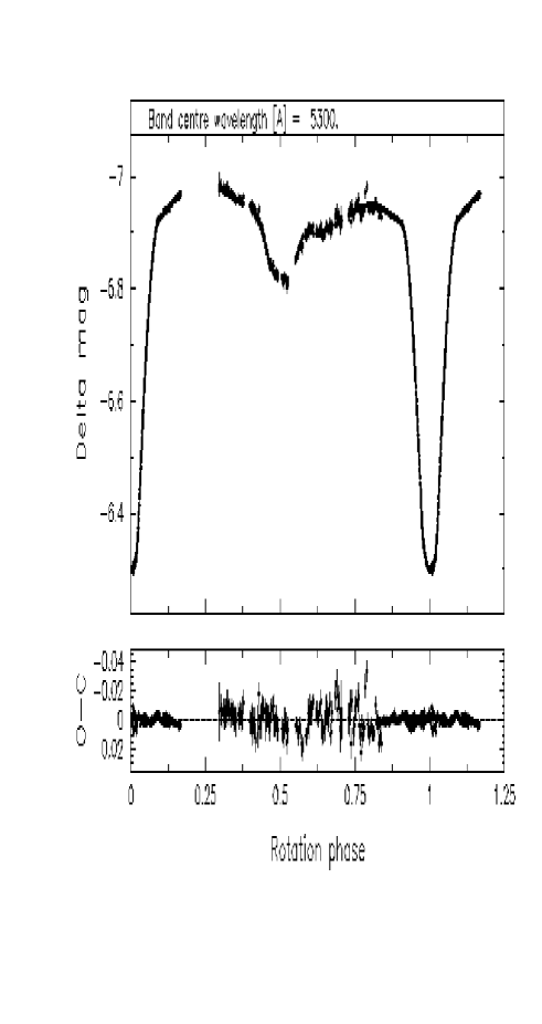
Figure 10: Combined HST and JGT lightcurves, with a Maximum Entropy fit with a polar cap and reduced photospheric temperature included.

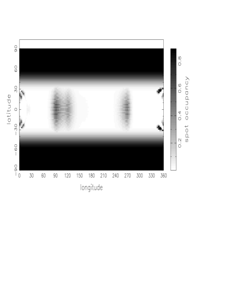
Figure 11: The final spot map of SV Cam (HST + JGT data) with two 46.7^∘ polar caps and reduced photospheric temperature. Note that phase runs in reverse to longitude. Spots reconstructed using $\chi^{2}$ and located at the quadrature points have been shown by Jeffers (2005) to be spurious as they can be reconstructed from models of high starspot coverage. Note that phase runs in reverse to longitude.

Figure 12: Observed minus Computed residuals for the case with a reduced photospheric temperature and a polar cap of 46.69^∘ radius. The four contact points are shown as vertical lines.

5.3 Final Lightcurve Fit

The best fitting stellar parameters are used to create a Maximum Entropy lightcurve fit (Fig. 10) and stellar surface brightness image for the primary star (Fig. 11). The observed data minus computed lightcurve residual for the primary eclipse, as shown in Fig. 12, is significantly flatter than the residuals shown in Fig. 5. The secondary eclipse shows also a better fit than in Fig.4. The reduced $\chi^{2}$ value after 25 iterations was 2.05, which is slightly reduced from the value of 3.55 obtained without a polar spot and a reduced photospheric temperature. This result shows that the presence of a polar cap and sub-resolution spots have a significant influence on the O-C residuals.

The Maximum Entropy surface brightness distribution, as shown in Fig. 11, is similar to that shown in Fig. 6. The spot feature at 0^∘ and 360^∘ is not an artifact as it is in the eclipse path of the secondary, but results from time variable structure in the base of the primary eclipse. It is a symmetric spot feature as image reconstructions from photometry are not able to determine a spot’s latitude. The spot feature at 25^∘ and 335^∘ in Fig. 6 has disappeared due to the correct determination of the primary star’s temperature and consequently the secondary star’s radius.

6 Discussion and Conclusions

We have used eclipse mapping, based on the maximum entropy method to recover images of the visual surface brightness distribution of the primary component of the RS CVn eclipsing binary SV Cam. It is only with the unprecedented photometric precision of the HST data that it is possible to see strong discontinuities at the four contact points in the residuals of the fit to the lightcurve. These features can only be removed from the O-C lightcurve by the reduction of the photospheric temperature, to synthesise high unresolvable spot coverage, and the inclusion of a polar spot.

In fitting SV Cam’s lightcurve we used the independently determined primary and secondary temperatures, as determined by Jeffers et al. (2005), as input to our solution. The primary and secondary radii were then determined using a ‘grid search’ method. Although the ‘grid search’ method is computationally intensive, it does provide reliable results. In contrast to this is the ‘downhill simplex’ amoeba method (Press et al., 1992) which repeatedly returned lightcurve solutions from local $\chi^{2}$ minima rather than from the global $\chi^{2}$ minimum. The resulting parameters (R_pri=1.238R_⊙ and R_sec=0.794R_⊙) are in closest agreement with the values of Pojmanski (1998) derived from spectroscopic data (R_pri=1.25R_⊙ and R_sec=0.8R_⊙). The errors derived in this work are an order of magnitude smaller than previous lightcurve solutions.

The Maximum Entropy fit to the data using the best-fitting orbital parameters shows strong discontinuities at the four contact points of the primary eclipse. When we reconstructed an image using only the ground based JGT data (photometric precision = 0.006) we found that these strong discontinuities were not visible in the residual lightcurve. It is only with the high photometric precision of the HST (0.00015 mag. or S/N 5000) that it is possible to distinguish the strong discontinuities in the residual lightcurve.

The surface brightness distribution shows spots at the quadrature points consistent with surface images of other RS CVns reconstructed using $\chi^{2}$ minimisation e.g. Olah et al. (1991) and Lanza et al. (2001), Lanza et al. (2002). However, the reliability of these images has been investigated by Jeffers (2005) where spurious spots at the quadrature points have been reconstructed from a synthetic star containing a high degree of sub-resolution spots. This is consistent with results from other methods such as TiO-band monitoring (O’Neal et al., 1998) which indicate that between 30% and 50% of a star’s surface could be covered in starspots at all times.

A high total spot coverage on SV Cam’s primary star will modify the apparent photospheric temperature. In a related paper Jeffers et al. (2005) showed that when the surface flux in the low-latitude eclipsed region was approximately 30% lower than the the best fitting phoenix model atmosphere. In this paper we showed that this is equivalent to a reduction in the photospheric temperature from 6039$\pm$58 K to 5935$\pm$38 K. High spot coverage also has important structural implications. As investigated by Spruit & Weiss (1986), a star with high spot coverage will, over thermal timescales, readjust its structure to compensate in radius and temperature. For example the primary star’s radius is 10% larger than expected for its spectral type, and could provide an explanation as to the large variation in binary system parameters as shown in Table 2.

The addition of a polar spot and the reduction of the photospheric temperature has a negligible influence on the empirically determined radius of the primary star, but a more significant influence on the secondary, decreasing it from 0.794$\pm$0.007 R_⊙ to 0.727$\pm$0.009 R_⊙. The presence of a polar spot will increase the depth of the primary eclipse, while a reduction in the photospheric temperature will decrease the depth of the eclipse. In both cases the binary system compensates for this by making the secondary star smaller as it consequently needs to eclipse less light. The standard luminosity-radius-temperature relation (L=4$\pi$R²$\sigma$T⁴) shows that if T_pri and T_sec are fixed the only variable parameters are the radii of the primary and secondary stars. The timing of the first and fourth contact points fixes the primary radius, leaving the secondary radius as the only adjustable parameter.

The resulting residuals from the Maximum Entropy lightcurve fit are significantly flatter with the lightcurve solution that includes a polar cap and a reduced photospheric temperature. However, there are still variations in the residual lightcurve, which could result from the eclipse mapping routine interpreting small scale variations in the lightcurve (i.e. unfitted spots) as noise. A 0.005 change magnitude as shown in Fig. 12 would result in additional 14% of the area of the annulus around the secondary being spotted than is shown in the surface brightness images. However, the remaining structure in the O-C residual could result from an incorrect value of the limb darkening or the presence of plage on the primary star’s surface, which will require further investigation.

The surface brightness image reconstructed with the refined binary system parameters (Fig. 11) has reduced surface structure compared to the image reconstructed with the original parameters. This is noticeable at longitudes 25^∘ and 335^∘, where the small spots have disappeared with the refined binary system parameters. The structure at longitudes 0^∘ and 360^∘ are not artifacts of the eclipse mapping technique as they are in the eclipse path of the secondary, but result from time variable structure on the surface of the primary star during primary eclipse. The features are symmetric as it is not possible to resolve a starspots latitude using photometric observations. Doppler images of active stars show that polar caps do not have a uniform structure, unlike the polar caps used in our model and shown in Fig. 11.

The upcoming COROT and KEPLER missions, which are designed to detect transits eclipses of stars by terrestrial sized planets, will discover thousands of eclipsing binary stars with micromag photometry, while missions such as GAIA should deliver 10⁶ new eclipsing binary stars. The benefit of such a wealth of high precision data will be lost if it is not possible to accurately solve the binary system parameters from the lightcurves.

References

- Albayrak et al. (2001) Albayrak B., Demircan O., Djurašević G., Erkapić S., Ak H., 2001, A&A, 376, 158
- Allard et al. (2000) Allard F., Hauschildt P. H., Schweitzer A., 2000, ApJ, 539, 366
- Bell et al. (1993) Bell S., Hilditch R., Edwin R., 1993, MNRAS, 260, 478
- Budding & Zeilik (1987) Budding E., Zeilik M., 1987, ApJ, 319, 827
- Collier Cameron (1997) Collier Cameron A., 1997, MNRAS, 287, 556
- Collier Cameron & Hilditch (1997) Collier Cameron A., Hilditch R. W., 1997, MNRAS, 287, 567
- Guthnick (1929) Guthnick P., 1929, Astron. Nachr., 235, 83
- Hilditch et al. (1979) Hilditch R. W., McLean B. J., Harland D. M., 1979, MNRAS, 187, 797
- Jeffers (2005) Jeffers S. V., 2005, MNRAS, 359, 729
- Jeffers et al. (2002) Jeffers S. V., Barnes J. R., Collier Cameron A., 2002, MNRAS, 331, 666
- Jeffers et al. (2005) Jeffers S. V., Cameron A. C., Barnes J. R., Aufdenberg J. P., Hussain G. A. J., 2005, ApJ, 621, 425
- Kjurkchieva et al. (2002) Kjurkchieva D. P., Marchev D. V., Zola S., 2002, A&A, 386, 548
- Lanza et al. (2002) Lanza A. F., Catalano S., Rodonò M., İbanoǧlu C., Evren S., Taş G., Çakırlı Ö., Devlen A., 2002, A&A, 386, 583
- Lanza et al. (2001) Lanza A. F., Rodonò M., Mazzola L., Messina S., 2001, A&A, 376, 1011
- Lehmann et al. (2002) Lehmann H., Hempelmann A., Wolter U., 2002, A&A, 392, 963
- Olah et al. (1991) Olah K., Hall D. S., Henry G. W., 1991, A&A, 251, 531
- O’Neal et al. (1998) O’Neal D., Neff J., Saar S., 1998, ApJ, 507, 919