Hubble Space Telescope Observations of SV Cam: II. First Derivative Lightcurve Modelling using phoenix and atlas Model Atmospheres

Abstract

The variation of the specific intensity across the stellar disc is essential input parameter in surface brightness reconstruction techniques such as Doppler imaging, where the relative intensity contributions of different surface elements are important in detecting starspots. We use phoenix and atlas model atmospheres to model lightcurves derived from high precision (S/N $\simeq$ 5000) HST data of the eclipsing binary SV Cam (F9V + K4V), where the variation of specific intensity across the stellar disc will determine the contact points of the binary system lightcurve. For the first time we use $\chi^{2}$ comparison fits to the first derivative profiles to determine the best-fitting model atmosphere. We show the wavelength dependence of the limb darkening and that the first derivative profile is sensitive to the limb-darkening profile very close to the limb of the primary star. It is concluded that there is only a marginal difference ($<$ 1$\sigma$) between the $\chi^{2}$ comparison fits of the two model atmospheres to the HST lightcurve at all wavelengths. The usefulness of the second derivative of the light-curve for measuring the sharpness of the primary’s limb is investigated, but we find that the data are too noisy to permit a quantitative analysis.

1 Introduction

Limb darkening effects in stellar atmospheres have important implications throughout stellar astrophysics where a determination of the surface brightness distribution is important. Recent work using Doppler imaging and micro-lensing events has shown that commonly-used analytical limb darkening laws fail to match stellar observations at the limb of the star (Thurl et al., 2004; Barnes et al., 2004). Other micro-lensing results (Fields, 2003) show that the intensity predictions from model atmospheres are discrepant in the case of a K-giant.

Surface brightness reconstruction techniques such as Doppler imaging and eclipse mapping rely on the information content of surface areas with different distances from the rotation axis (see review by Collier Cameron (2001)). To detect starspots Doppler imaging uses the relative intensity contributions, calculated from model atmospheres, of the different surface elements. To reconstruct an accurate surface brightness distribution it is essential to know how parameters, such as the limb darkening, can alter the intensity values across the stellar disc.

High inclination eclipsing binary systems can be used as probes to determine the variation of specific intensity at the stellar limb. If limb darkening showed a smooth transition in specific intensity at the limb of the star, the contact points of eclipses would appear less abrupt and slightly displaced in phase relative to models with limb darkening laws derived from plane-parallel atmospheres, where the cutoff is very sharp. The sharp cutoff in plane parallel atmospheres results from the optical depth of the rays being infinite at the limb.

In November 2001 we were awarded 9 orbits of HST/STIS time to eclipse-map the inner face of the F9V primary of the totally eclipsing binary SV Cam. SV Cam (F9V + K4V) is a synchronously rotating RS CVn binary with a period of 0.59d. We obtained spectrophotometric lightcurves of 3 primary eclipses with a signal-to-noise ratio of 5000. The first analysis of these data, by Jeffers et al. (2005), determined the radii of the primary and secondary stars. When the resulting lightcurve was subtracted from the observed data, the residual lightcurve showed strong peaks at phases of contact. Jeffers et al. (2005) then showed that these mismatches are reduced significantly, but not eliminated, when a polar cap and a reduction in the photospheric temperature, to synthesise high spot coverage, are imposed on the image.

As there is a significant temperature difference between the primary and secondary stars, the secondary star acts as a dark occulting disc as it eclipses the primary star. The variation of brightness as a function of phase reflects the degree of limb darkening on the primary star. In this paper we determine the best fitting model atmosphere by fitting the models to the brightness variations as the secondary scans the inner face of the primary star, using the first and second derivatives of the HST in 10 wavelength bands. We discuss the implications these results have on results from Doppler Imaging.

2 Model atmospheres

In this paper, two well established stellar atmosphere codes are used; the phoenix model atmosphere code (Hauschildt et al., 1999) that uses spherical atmospheres and the atlas model atmosphere code (Kurucz, 1994) that uses plane parallel atmospheres.

2.1 atlas

We use the plane-parallel ATLAS9 model atmospheres from the Kurucz CD-ROMS (Kurucz, 1994). We integrate the intensity values over the wavelength range of our observations 2900Å to 5700Å. We use temperature models from 3500 K to 6500 K, with 250 K interval, across 17 limb angles. The limb angle $\mu$ is defined by $\mu$= cos $\theta$, where $\theta$ is the angle between the line of sight and the normal vector of the local surface element. The treatment of convection is based on the mixing length theory with approximate overshoot (ref. Castelli et al. (1997)) with a mixing length to scale height ratio of 1.25. The variation of specific intensity, i.e. at $\mu$=1,as a function of wavelength and limb angle is shown in Figure 1.

2.2 phoenix

The general input physics set-up of the phoenix model atmosphere code is discussed in Hauschildt et al. (1999). The main advantage of using this code is that it is based on spherical geometry (spherical radiative transfer) LTE rather than traditional plane-parallel structure. NLTE effects are considered to be insignificant in this application.

The synthetic spectra are based on an extension of the grid of PHOENIX model atmospheres described by Allard et al. (2000). This extended grid includes surface gravities larger than $\log(g)>3.0$ needed for main sequence stars. These models are as described by Hauschildt et al. (1999), but include an updated molecular line list. The models are computed in spherical geometry with full atomic and molecular line blanketing using solar elemental abundances. In these models, the stellar mass is 0.5 M_⊙ and the convection treatment assumes a mixing-length to pressure scale height ratio of 2 with no overshooting. There are 117 synthetic spectra in total. The effective temperature runs from 2700K to 6500 K in 100K steps at three surface gravities: $\log(g)$ = 4.0, 4.5, and 5.0. The wavelength resolution of these synthetic spectra is 1Å.

The variation of specific intensity as a function of limb angle is shown in Figure 1. The difference between the phoenix and the atlas model atmospheres at the limb of the star results primarily from the effects of spherical geometry of the phoenix model. In models using spherical geometry, there is a finite optical depth for rays close to the limb, while with plane parallel models the optical depth of the rays is infinite at the limb providing significant intensities down to $\mu$=0. Other contributing effects include overshooting and the mixing length ratio.

In addition to the limb effects, Fig. 1 shows that atlas intensity profiles are overall brighter than phoenix intensity profiles. We attribute this difference to the use of overshooting in the atlas models. atlas models with overshooting have been shown to have weaker limb darkening in the blue relative to models without overshooting, for instance, overshooting models have been shown to better fit solar limb darkening observations than non-overshooting models Castelli et al. (1997). A similar result holds for Procyon (F5 IV-V); ref. Aufdenberg et al. (2005) for a detailed study of the effects of 1-D and 3-D convection on limb darkening.

Figure 1: The predicted variation in specific intensity across the stellar disc as a function of wavelength for the longest (5596Å) and the shortest (3198Å) wavelengths in this analysis (T=6000 K, log g=4.5).

2.3 Model lightcurves

We use the eclipse-mapping code DoTS (Collier Cameron, 1997) to model the primary eclipse lightcurve for each model atmosphere, and to determine which model atmosphere best fits the complete HST lightcurve. The input data to each model comprises: the variation of the specific intensity as a function of limb angle, as shown in Figure 1 for both model atmospheres considered; the primary and secondary radii; a reduced primary photospheric temperature and polar spot. Gravity darkening is also included according to the description of Collier Cameron (1997).

We include a reduced photospheric temperature to account for a stellar surface that is peppered with small spots which are too small to be resolved through eclipse mapping. Following the results of Jeffers et al. (2005) we include a polar cap in the modelled lightcurve to optimise the fit of the lightcurve to the data. The method for modelling the photometric lightcurve to include a reduced photospheric temperature and a polar cap is described in Appendix A for the atlas model atmosphere. The binary system parameters are summarised in Table 2. The lightcurve solutions for the two model atmospheres are in good agreement.

3 HST Observations

Visit	Obs. Date	UT	UT	Exposure	No of
		Start	End	Time(s)	Frames
1	01 November 2001	20:55:56	01:00:17	30	165
2	03 November 2001	14:34:29	18:38:21	30	165
3	05 November 2001	09:49:17	13:52:22	30	165

Table 1: HST Observations of SV Cam, where the exposure time is per frame.

Three primary eclipses of SV Cam were observed by the HST, using the Space Telescope Imaging Spectrograph with the G430L grating. The observations used 9 spacecraft orbits and spanned 5 days at 2 day intervals from 1-5 November 2001 as shown in Table 1. Summing the recorded counts over the observed wavelength range 2900 Å  to 5700 Å yields a photometric lightcurve. Figure 2 shows the photometry of the 3 eclipses observed during the 9 orbits. The observations have a cadence of 40s and a photometric precision of 0.0002 magnitudes (S:N 5000) per 30 s exposure. The observations and the data reduction method are explained in greater detail in Jeffers et al. (2005).

Figure 2: The comprising sections of the primary eclipse from each of the 3 HST visits. The flux density has been summed between 2900 Å  and 5700 Å. An off-set of 4$\times$10⁶ ergs/s/cm² has been added for clarity.

Model Grid	Log g	L/H	Fitted	Spotted	Primary	Secondary	Polar Spot
			Temp (K)	Temp. (K)	Radius (r⊙)	Radius (r⊙)	(degrees)
phoenix	4.5	2.0	6038$\pm$58	5935 $\pm$28 K	1.235 $\pm$ 0.003	0.727 $\pm$ 0.003	46.5 $\pm$ 8
atlas	4.5	1.25	5972$\pm$59	5840 $\pm$53 K	1.241 $\pm$ 0.003	0.729 $\pm$ 0.002	45.7 $\pm$ 9

Table 2: Geometric binary system parameters computed for SV Cam with a reduced photospheric temperature due to the star being peppered with small spots, and increased radii due to the presence of a polar cap. L/H is the mixing-length to pressure scale height ratio

4 Wavelength dependence of limb darkening

Figure 3: The variation of the HST lightcurve with wavelength. Each lightcurve has been plotted with an offset of 5 $\times$ 10^-12 from the lightcurve at the bottom of the plot (3198 Å).

Figure 4: HST lightcurves with the longest (5596 Å) and shortest wavelengths (3198 Å), showing the variation of limb darkening with wavelength and the temporal evolution of bright magnetic features over the 5 day timespan our observations. The variation in the 3198Å band is of the order of 5%.

Figure 5: First derivative profiles for each of the 10 HST lightcurves as plotted in Figure 3. The presence of a bright magnetic feature is the cause of the variation in waveband 3198Å.

Figure 6: First derivative profiles, constructed with the same stellar parameters as in Figure 5, but with no limb darkening. The slight negative slope during total eclipse results from a non-spherical star caused by tidal interactions in the binary system.

Figure 7: First derivative profiles of the observed lightcurve of wavelengths 5596 Å and 3707 Å  for total eclipse, i.e. between second and third contact, showing the variation of limb darkening with wavelength.

Figure 8: First derivative profiles for the longest (5596 Å) and shortest wavelengths (3198 Å), as plotted in Figure 5, using intensities interpolated from the phoenix grid at the best fit effective temperature and gravity shown in Table 2.

Figure 9: First derivative profiles for with the longest (5596 Å) and shortest wavelengths (3198 Å), using intensities interpolated from the atlas grid at the best fit effective temperature and gravity shown in Table 2.

The variation of the HST lightcurve with wavelength was determined by phasing the three primary eclipses together and dividing each spectrum into 10 bands of equal flux, as shown in Figure  3. The increased fluctuations at shorter wavelengths are consistent with the presence of signatures bright magnetic activity, as they are strongest in the bluest wavelength band. The fluctuations at blue wavelengths are not a short-timescale phenomenon, but rather a mismatch in flux levels arising from a change in the star’s UV flux from second to third visit.

The curvature of the eclipse profile between second and third contact illustrates clearly that limb darkening increases to wards shorter wavelengths. The wavelength dependence of limb-darkening is revealed by the models collected by Claret (2000), but more fundamentally by direct observations of the Sun, for example Neckel & Labs (1994). Both the brightness variation and the variation of the limb darkening with wavelength are illustrated by plotting the bluest and reddest wavelength bands, as shown in Figure 4.

5 First Derivative Profiles of Lightcurves

5.1 Basic properties

As the primary star dominates the light of the binary system, the cooler secondary acts as a dark occulting disc scanning across the equatorial region of the primary during eclipse. The variation of the specific intensity as a function of limb angle across the primary star shows the degree of limb darkening.

To determine the optimally fitting model atmosphere to the HST lightcurves it is necessary to examine the degree of curvature in the eclipse profile. We use the first derivative, with respect to phase, of the lightcurves to determine the rate of change of the eclipsed flux with phase. This is the first time that this method has been applied to photometric data of an eclipsing binary system. The numerical derivative is computed using the Interactive Data Language (IDL) routines deriv and derivsig which employ 3-point Lagrangian interpolation.

The profiles of the first derivative for each of the 10 HST wavebands are shown in Figure 5. The first contact point is at phase 0.906$\pm$0.003, the second contact point is at phase 0.977$\pm$0.003, the third contact point is at 1.023$\pm$0.003, and the fourth contact point is at 1.093$\pm$0.003. The gradient of the first derivative profile between second and third contact points is indicative of the degree of limb darkening in the lightcurve. In the first derivative of the model with no limb darkening, this region the profile is flat (Figure 6). The variation of limb darkening with wavelength is illustrated in Figure 7, where the first derivative lightcurves from the longest wavelength (5596 Å) and the second shortest wavelength (3707 Å) are plotted between the second and third contact points. The first derivative profile of the shortest wavelength contains too much deviation, caused by a bright feature on the primary’s surface, to provide a clear example.

The variation of the first derivative profile with wavelength is also visible in the profile using the phoenix model atmosphere, as shown in Figure 8. In contrast to this Figure 9 shows the same first derivative profiles based on the atlas model atmosphere. In the atlas first derivative profiles there is more variation between the two wavelength bands than in the phoenix model atmosphere. The variation with wavelength relates directly to the variation of specific intensity with wavelength as previously shown in Figure 1.

5.2 First derivative lightcurve fitting

The first derivative profiles of the HST observations, in each of the 10 wavelength bands (Figure 5), are fitted using reduced $\chi^{2}$ comparison fits to the first derivatives of the phoenix and atlas model atmospheres of the same wavelength as the observations. In this analysis the larger error bars are those of the models, given the large uncertainties shown in Table 2, and the finite number of planer elements used in the modelling of the lightcurves. We estimate these errors to be of the order of 1%.

The fits to the observations are determined using (i) the totally eclipsed section of the lightcurve between second and third contact points only, and (ii) the region of the eclipse between the first and fourth contact. Figure 10, and Figure 11, respectively show the results for case (i) and (ii) at the wavelength 4535 Å. The $\chi^{2}$ values for all of the lightcurves are summarised in Table 3.

The results show that between first and fourth contact phoenix gives the best fit, except for the wavelength band centred at 3198Å and 3707Å. However, the best fitting model in the region of total eclipse between second and third contact shows a wavelength dependence. For wavebands centred at 4313Å, 4539Å, and 4743Å atlas provides the best fit, while phoenix is the best fitting model atmosphere at shorter and longer wavelengths.

Wavelength	phoenix(1)	atlas(1)	phoenix(2)	atlas(2)
3198	367.27	374.69	285.64	286.85
3707	8.41	8.82	7.73	7.66
4052	5.82	7.19	6.12	6.39
4313	5.70	5.49	4.90	5.26
4539	4.84	4.93	4.81	5.11
4753	5.00	4.21	5.04	4.81
4952	6.08	5.57	4.56	4.83
5169	4.60	5.56	4.53	5.11
5384	4.50	4.55	4.91	5.25
5598	5.09	5.53	6.62	7.06

Table 3: Best fitting reduced $\chi^{2}$ values for lightcurves fitted in the regions in the primary eclipse profile between (1) first and fourth contact, and (2) second and third contact. This table is graphically shown in Figures 13.

Figure 10: The first derivative profile centred at 4539Å, plotted with the phoenix and atlas model atmospheres. The phase range is between second and third contact. The lower plot shows the residual (observations - model) of this fit.

Figure 11: The first derivative profile centred at 4539Å, plotted with the phoenix and atlas model atmospheres. The phase range is between first and fourth contact.

Figure 12: The second derivative profile using the complete HST lightcurve, plotted with the phoenix and atlas model atmospheres.

Figure 13: The variation of reduced $\chi^{2}$ as a function of wavelength for phases between second and third contact (top) and first and fourth contact (bottom) as tabulated in Table 3.

6 Second derivative lightcurve fitting

As with taking the first derivative of the lightcurve to determine the rate of change of the slope in the eclipse profile, we now determine the rate of change of the first derivative profile, i.e. the second derivative of the eclipse profile. The signal-to-noise ratio of the observed data set was insufficient to determine useful second derivative profiles for each of the 10 HST lightcurves. Instead we take the second derivative of the complete HST lightcurve and fit phoenix and atlas model atmospheres centred at 4670Å. We fit the second derivative profile between first and fourth contact as between second and third contact we would only fit numerical noise.

The best fitting model atmosphere is phoenix with a relative $\chi^{2}$ of 7.02, while the atlas model atmosphere has a relative $\chi^{2}$ of 8.73. The fit to the second derivative profile for the phoenix and the atlas model atmospheres are shown in Figure 12. The jitter in the models is caused by numerical noise arising from the finite number of planar surface elements used to model the star in the synthesis code.

7 Discussion and Conclusions

The best-fitting geometric parameters determined using phoenix and atlas model atmospheres are in good agreement. As shown in Figure 1, the predicted specific intensity for the atlas models is greater at the limb than for phoenix models, which will consequently make the primary star bigger. To compensate for this the best-fitting temperature of the primary star is slightly cooler than fitted using phoenix models. In this analysis we solved the geometric system parameters of the lightcurve using complete lightcurve rather than solving the parameters individually for each of the 10 sub-lightcurves. From Figure 1, we would expect the best-fitting radii, solved using phoenix and atlas, to be closer at redder wavelengths than at bluer wavelengths, but would not differ enough to alter the conclusions of this analysis.

We have shown the wavelength dependence of limb darkening by sub-dividing the HST lightcurve into 10 bands of equal flux. The variation of flux between first and fourth contact shows that the limb darkening decreases towards longer wavelengths, confirming published limb darkening values, for example by Claret (2000), and as observed on the Sun Neckel & Labs (1994) and interferometrically in K-giants by Mozurkewich et al. (2003). The splitting of the HST lightcurve into 10 wavelength bands also highlights the presence of a time variable bright bright feature, possibly an active region or plage on the surface of the primary star, visible in the bluest wavelength band (3198Å). The temporal variation of the bright feature is of the order of 3 days as it comes into view on the primary star between the second and third HST visit.

The ratio of the temperatures of the two stars has the effect that the secondary star acts as a dark occulting disc that scans the surface of the primary star. During partial eclipse (i.e. between first and second, and third and fourth contacts) the curvature of the lightcurve provides information about the variation of the specific intensity with limb angle of the primary star. During total eclipse the curvature of the lightcurve provides information on the variation of specific intensity as a function of limb angle. The first derivative profile for each of the 10 HST wavelength bands clearly indicates the change in slope as a function of phase. Figure 7 shows the wavelength variation of the gradient of the first derivative profile of the HST lightcurves centred at 3707Å and 5596Å. The slope of the shorter wavelength is steeper than for the longer wavelength, consistent with the limb darkening decreasing towards longer wavelengths.

The best fitting model atmosphere is determined using $\chi^{2}$ comparison fit. The first derivative profile of the modelled lightcurves, generated with phoenix and atlas model atmospheres, was fitted to the HST lightcurves. The results show that the majority of the results differ by less than 1$\sigma$ making the differences between the two models largely insignificant.

Surface brightness reconstruction techniques such as Doppler imaging, and eclipse mapping rely on the information content of surface areas with different distances from the rotation axis (see review by Collier Cameron (2001)). To detect starspots Doppler imaging uses the relative intensity contributions, calculated from model atmospheres, to represent the different surface elements. To reconstruct an accurate surface brightness distribution it is essential to know how parameters, such as the limb darkening, can alter the intensity values across the stellar disc. To date there are many surface brightness images reconstructed using Doppler imaging and eclipse mapping techniques on stars with similar spectral types to SV Cam. Examples include: He699, G2V (Jeffers et al., 2002), AE Phe G0V+F8V (Barnes et al., 2004), Lu Lup, G2V (Donati et al., 2000) and R58, G2V (Marsden et al., 2005), reconstructed using atlas plane-parallel model atmospheres. The lightcurve modelling results of this work clearly show that there is no distinguishable difference between the two models using the high signal-to-noise SV Cam observations.

The first derivative profiles show a small excess in the observed flux at phase $\approx$ 0.9825 (just after second contact), compared with the fitted model atmospheres. In contrast, there is a slight decrease in the observed flux at phase 1.015, i.e. just before third contact. The increase and decrease of the first derivative at these points could be evidence for an additional emission. As this light excess is located just before the second contact point, and the reverse just before the third contact point, it could indicate that the very edge of the secondary’s limb is transparent to the light of the primary star.

The signal-to-noise ratio of this data set was not high enough to determine useful second derivative profiles for each of the 10 HST lightcurves. Instead we take the second derivative of the complete HST lightcurve and fit phoenix and atlas model atmospheres centred at 4670Å to the observed lightcurve. The jitter in the models is caused by numerical noise arising from the finite number of planar surface elements used to model the star in the synthesis code. We fit the lightcurve between first and fourth contact as there is insufficient structure to fit between second and third contact. The results show that the phoenix model atmosphere code gives a marginally better fit at the limb of the star. However, phoenix does not provide an exact fit, which could indicate that the observed cut-off in the limb intensity is steeper than predicted. This could explain why Jeffers et al. (2005) could not completely remove the strong discontinuities in the observed minus computed residual.

Appendix A Determination of the percentage of spot coverage and polar cap temperature for ATLAS model atmospheres

In this appendix we describe the method used to determine the reduced photospheric temperature due to the presence of many unresolvable spots and the polar cap size, as quoted in Table 2 for the ATLAS model atmospheres. In a related paper, Jeffers et al. (2005) showed that in order to fit the HST lightcurve of SV Cam it was necessary to reduce the photospheric temperature, to mimic the peppering of the primary star’s surface with small starspots, and to include a polar cap. In this appendix we determine the best-fitting lightcurve solution to the SV Cam lightcurve using atlas model atmosphere. It is important to do this to not to introduce an inherent bias to the results of this paper.

A.1 Unresolved spot coverage

In this section determine the unresolved spot coverage, following the method of Jeffers et al. (2005). We assume that the unresolved spot coverage comprises many small spots peppering the primary star, and a polar cap which is not possible to resolve from a photometric lightcurve.

A.1.1 Temperature Fitting

In the method of Jeffers et al. (2005) the combination of the SV Cam lightcurve and the Hipparcos parallax is used to determine the primary and secondary temperatures. Knowing the radii of the two stars we can evaluate the flux contribution from the secondary star relative to that of the primary star. The best-fitting combination of primary and secondary temperatures is determined using $\chi^{2}$ minimisation, where a scaling factor $\gamma$ is included to ensure that the shape of the spectrum is fitted rather than the absolute flux levels. The resulting $\chi^{2}$ landscape plot is shown in Figure 14. The minimum value occurs at 5973$\pm$31 K and 4831$\pm$103 K for the primary and secondary stars respectively.

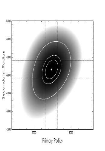
Figure 14: Contour plot of the $\chi^{2}$ landscape of the combined primary and secondary stars. The minimum $\chi^{2}$ value occurs at 5973 $\pm$ 31 K, and 4831 $\pm$ 103 K, for the primary and secondary stars respectively. From the centre of the plot the first contour ellipse represents the 1 parameter 1 $\sigma$ confidence limit at 63.8%, the second ellipse represents the 2 parameter 1 $\sigma$ confidence limit at 63.8% whilst the third ellipse represents the 2 parameter 2.6 $\sigma$ 99% confidence limit.

The temperature of the primary star is then determined by isolating the primary star’s spectrum. To achieve this we subtracted a spectrum outside of the primary eclipse from one inside of the eclipse which results in the spectrum of the primary star but with the radius of the secondary star. The temperature is fitted using $\chi^{2}$ minimisation, where the minimum temperature is determined by a parabolic fit. This results in a minimum primary temperature of 5872$\pm$59 K (Figure 15), with the errors determined by setting $\Delta\chi^{2}$=1.

Figure 15: Parabolic fit to determine the primary temperature minimum to be 5872$\pm$53 K

A.1.2 Fractional Starspot Coverage

Following the conclusions of Jeffers et al. (2005) we attribute the missing flux to be indicative of small unresolvable spots on the primary star’s surface. The dark starspot filling factor is given by:

$$\alpha=1-\gamma$$ (1)

where $\alpha$ is the fractional starspot coverage and $\gamma$ is the scaling factor. The interpolated scaling factor for the primary temperature is determined as shown in Figure 16. The scaling factor is 0.76, resulting in a fractional coverage of dark starspots of 24%.

Figure 16: Scaling factor ($\gamma$) as a function of Primary Temperature (atlas models). The scaling factor for T=5872 K is determined by a quadratic fit to these points.

A.1.3 Polar Cap

The determination of the spot coverage fraction only accounts for the flux deficit in the eclipsed equatorial latitudes of the primary star. Extending the 24% spot coverage to the entire surface of the primary star (as described by (Jeffers et al., 2005)) we find that there is an additional 13.5% flux deficit. The binary eclipse-mapping code DoTs is used to model artificial polar spots on the surface of SV Cam, to include effects resulting from the star being a sphere and not a disc, limb and gravity darkening and spherical oblateness. We model the fractional decrease in stellar flux as a function of polar spot size and determine the polar spot radius to be 43.5$\pm$6^∘ (Fig.  17).

Figure 17: Fractional decrease in the stellar flux of SV Cam as a function of theoretical polar cap size

A.2 Lightcurve Modelling

To compare ATLAS and PHOENIX model atmospheres we need to determine the best-fitting binary system parameters to the observed SV Cam lightcurve for each model atmosphere separately to avoid introducing a an inherent bias to our results. We include the presence of high unresolvable spot coverage and polar caps in the lightcurve fit by using the method of Jeffers et al. (2005). Such spot coverage has been shown by that method to have a significant impact on the binary system parameters.

A.2.1 Reduced Photospheric Temperature

The peppering of small starspots poses a limitation on image reconstruction techniques from photometric lightcurves such as Maximum Entropy eclipse mapping (Jeffers, 2005). To model the presence of many dark unresolvable starspots we decrease the apparent photospheric temperature of the star. To determine the reduction in the photospheric temperature of the star we model starspot distributions equating to 1.8%, 6.1%, 18%, 48% and 100% of the stellar surface on an immaculate SV Cam. For each model the initial photospheric temperature is 5904 K and the spot temperature is 4400 K. Each of these starspot distributions is modelled as a photometric lightcurve. Using the Maximum Entropy eclipse mapping method we determine the best-fitting temperature to each model lightcurve using a $\chi^{2}$ grid-search method. A quadratic fit to the best-fitting temperatures show that for a starspot coverage of 24%, the apparent photospheric temperature is 5840 K (Figure 18).

Figure 18: The decrease of the primary star’s apparent photospheric temperature as a function of the percentage of spot coverage on its surface.

A.2.2 Polar Cap

We include a polar cap in our analysis to verify the results in the previous section, following the method of Jeffers et al. (2005). The polar spot is assumed to be at 4500 K, circular, centred at the pole, and is in addition to the peppered spot distribution as described above. For each polar spot size (from 40^∘ to 50^∘) the minimum primary and secondary radii are determined using a $\chi^{2}$ contour map. These minimum $\chi^{2}$ values are plotted as a function of polar spot size in Figure 19. The best fitting polar cap size, 45.7^∘ was determined from the minimum of a quadratic function fitted to these points. The grid search of radii is repeated using a fixed value for the polar spot size. The results for the $\chi^{2}$ minimisation are summarised in Table 2 shown as a contour map in Figure 20.

Figure 19: Quadratic fit to the variation of $\chi^{2}$ as a function of polar spot size.

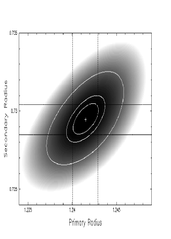
Figure 20: Contour plot of the $\chi^{2}$ landscape for the primary and secondary radii with a 45.7^∘ polar spot. From the centre of the plot, the first contour ellipse is the 1 parameter 1$\sigma$ confidence limit at 63.8%, the second contour ellipse is the 2 parameter 1$\sigma$ confidence limit at 63.8%, and the third contour ellipse is the 2 parameter 2.6$\sigma$ confidence limit at 99%.

A.3 Summary

We have shown in this section that the best fitting binary system parameters determined using the atlas model atmosphere are in agreement with those determined using phoenix model atmospheres (Jeffers et al., 2005). This further shows that at there is no significant difference between phoenix and atlas model atmospheres at the F9V+K4V spectral types. The results are summarised in Table 2.

References

- Allard et al. (2000) Allard F., Hauschildt P. H., Schweitzer A., 2000, ApJ, 539, 366
- Aufdenberg et al. (2005) Aufdenberg J. P., Ludwig H.-G., Kervella P., 2005, ApJ, 633, 424
- Barnes et al. (2004) Barnes J. R., Lister T. A., Hilditch R. W., Collier Cameron A., 2004, MNRAS, 348, 1321
- Castelli et al. (1997) Castelli F., Gratton R. G., Kurucz R. L., 1997, A&A, 318, 841
- Claret (2000) Claret A., 2000, A&A, 363, 1081
- Collier Cameron (1997) Collier Cameron A., 1997, MNRAS, 287, 556
- Collier Cameron (2001) Collier Cameron A., 2001, Lecture Notes in Physics, Berlin Springer Verlag, 573, 183
- Donati et al. (2000) Donati J.-F., Mengel M., Carter B., Marsden S., Collier Cameron A., Wichmann R., 2000, MNRAS, 316, 699
- Fields (2003) Fields D. L. et al., 2003, ApJ, 596, 1305
- Hauschildt et al. (1999) Hauschildt P. H., Allard F., Ferguson J., Baron E., Alexander D. R., 1999, ApJ, 525, 871
- Jeffers (2005) Jeffers S. V., 2005, MNRAS, 359, 729
- Jeffers et al. (2002) Jeffers S. V., Barnes J. R., Collier Cameron A., 2002, MNRAS, 331, 666
- Jeffers et al. (2005) Jeffers S. V., Cameron A. C., Barnes J. R., Aufdenberg J. P., Hussain G. A. J., 2005, ApJ, 621, 425
- Jeffers et al. (2005) Jeffers S. V., Collier Cameron A., Barnes J. R., Donati J. F., 2005, MNRAS in press
- Kurucz (1994) Kurucz R. L., 1994, CDROM # 19, Cambridge, MA
- Marsden et al. (2005) Marsden S. C., Waite I. A., Carter B. D., Donati J.-F., 2005, MNRAS, 359, 711
- Mozurkewich et al. (2003) Mozurkewich D., Armstrong J. T., Hindsley R. B., Quirrenbach A., Hummel C. A., Hutter D. J., Johnston K. J., Hajian A. R., Elias N. M., Buscher D. F., Simon R. S., 2003, AJ, 126, 2502
- Neckel & Labs (1994) Neckel H., Labs D., 1994, Solar Phys., 153, 91
- Thurl et al. (2004) Thurl C., Sackett P. D., Hauschildt P. H., 2004, Astron. Nachr., 325, 247