Relative velocities among accreting planetesimals in binary systems:
the circumprimary case

Manuscript Pages: 31

Tables: 4

Figures: 10

Proposed Running Head:planetesimal accretion in binaries

Editorial correspondence to:

Philippe Thébault

Stockholm Observatory

Albanova Universitetcentrum

SE-10691 Stockholm

Sweden

Phone: 46 8 5537 85 59

E-mail: philippe.thebault@obspm.fr

ABSTRACT

We investigate classical planetesimal accretion in a binary star system of separation $a_{b}\leq$50 AU by numerical simulations, with particular focus on the region at a distance of 1 AU from the primary. The planetesimals orbit the primary, are perturbed by the companion and are in addition subjected to a gas drag force. We concentrate on the problem of relative velocities $\Delta v$ among planetesimals of different sizes. For various stellar mass ratios and binary orbital parameters we determine regions where $\Delta v$ exceed planetesimal escape velocities $v_{esc}$ (thus preventing runaway accretion) or even the threshold velocity $v_{ero}$ for which erosion dominates accretion. Gaseous friction has two crucial effects on the velocity distribution: it damps secular perturbations by forcing periastron alignment of orbits, but at the same time the size–dependence of this orbital alignment induces a significant $\Delta v$ increase between bodies of different sizes. This differential phasing effect proves very efficient and almost always increases $\Delta v$ to values preventing runaway accretion, except in a narrow $e_{b}\simeq 0$ domain. The erosion threshold $\Delta v>v_{ero}$ is reached in a wide ($a_{b},e_{b}$) space for small $<10\,$km planetesimals, but in a much more limited region for bigger $\simeq 50\,$km objects. In the intermediate $v_{esc}<\Delta v<v_{ero}$ domain, a possible growth mode would be the type II runaway growth identified by Kortenkamp et al. (2001).

keywords planetary formation – planetary dynamics – accretion

1 INTRODUCTION

The problem of planetary formation in binary systems is a crucial one, as a majority of solar type stars are believed to reside in binary or multiple star systems. New light on this issue has been shed by the recent discoveries of several extrasolar planets around stars in binary systems (Eggenberger et al., 2003). In the classical planetary formation scenario, one crucial stage is the mutual accretion of kilometre-sized planetesimals leading, through runaway and possibly oligarchic growth, to the formation of lunar–to–Mars sized embryos on relatively short timescales of $5\times 10^{3}$ to $10^{5}\,$ years. (e.g. Greenberg et al., 1978; Wetherill & Stewart, 1989; Barge & Pellat, 1993; Lissauer, 1993; Kokubo & Ida, 1998, 2000; Rafikov, 2003, 2004). We focus here on the specific problem of planetesimal accretion around the circumprimary star under the perturbing influence of the companion. The crucial parameter for this stage is the encounter velocity between impacting objects, which has to be lower than the bodies escape velocity (corrected by an energy dissipation factor) in order to allow mutual accretion. In a gravitationally unperturbed disk, this condition is met for a large fraction of mutual impacts (e.g Safronov, 1969; Greenberg et al., 1978), but external gravitational perturbations might lead to relative velocity increase and thus inhibit accretion. Such a risk obviously exists in a binary system, where the companion star affects the inner disk through secular perturbations leading to substantial eccentricity oscillations (e.g. Marzari & Scholl, 2000; Thébault et al., 2004, hereafter TH04). However, these secular effects come with a strong forced orbital phasing between neighboring objects. This tends to keep relative velocities at a lower level than expected from using the usual approximation $\Delta v\propto e\,v_{kep}$, which is anyway often misleading (see for instance the discussion for the specific case of the Kuiper Belt in Thébault & Doressoundiram, 2003). Nevertheless, the secular oscillations get narrower with time so that at some point neighboring orbits eventually cross, leading to very high encounter velocities. This orbital crossing criterion has been explored analytically by Heppenheimer (1978), who used a simplified estimate for the apsidal line regression timescale. Whitmire et al. (1998) carried out a more detailed study by numerically integrating the orbits of the stars of the binary system and of two massless planetesimals over a typical runaway growth timescale of $2\times 10^{4}$ years. This study claims that, within the timescale of their numerical simulations, the main variations of the planetesimal orbital elements are due to short term effects of the binary gravity field that would be averaged out in a secular theory. However, it is not clear if their adopted methodology, i.e. extrapolating orbital crossing criteria from orbital parameters recorded only at binary periastron, allows to correctly estimate these short term intra-orbit effects. In addition, as the authors point out themselves, the choice of initial parameters and assumptions were made in order to get the most conservative criteria for orbital crossing, thus necessarily overestimating the short term effect’s efficiency. Furthermore, over $2\times 10^{4}$ years the secular perturbations have sufficient time to build up a dephasing $d\varpi$ in the longitude of periastron of two planetesimals. This $d\varpi$ depends on the initial difference in semimajor axis between the orbits of the two bodies. Unfortunately, it is difficult for their model to separate the contribution to the impact velocity of the short term effects from that coming from the dephasing of the secular perturbations. Finally, the potentially crucial effect of gas drag on relative velocity evolution was left out of this purely gravitational study.

We shall here adopt a different approach, based on the numerical scheme developed in earlier studies (e.g. Marzari & Scholl, 2000; Thébault et al., 2002, 2004) to study the encounter velocity evolution, within a test planetesimal population, under the coupled effect of dynamical perturbations and gaseous friction. These previous studies allowed us to identify and quantitatively study the onset of orbital crossing, and in particular its progressive wave-like inward propagation, as well as its damping by gas drag, for individual specific perturber configurations. We here intend to take these studies a step further and extend them to the general case of any given binary system configuration. In a first step, we investigate the purely gravitational problem which is the basis to understand more advanced results including gas drag. For this gas-free system, our numerical code is used to empirically derive analytical estimates of the orbital crossing location and of the induced encounter velocities increase. These general laws are expressed as a function of the free parameters here explored: the binary separation $a_{b}$, the companion’s eccentricity $e_{b}$ and its mass $m_{b}$. We pay particular attention to the timescale for the inward propagation of the orbital crossing “wave”. The second part of our work is devoted to the study of how gas drag affects these pure gravitation induced results. Frictional drag by the gas of the protoplanetary disk might indeed play an important role here. If efficient enough, it can restore the periastron alignment (e.g. Marzari & Scholl, 1998), preventing orbital crossing of orbits with different semimajor axes. At the same time, it partially damps the amplitude of oscillations in eccentricity induced by the companion star. Another important aspect of gas drag is that it is size dependent, and thus introduces differential effects between bodies of different radius (e.g. Marzari & Scholl, 2000; Kortenkamp et al., 2001; Thébault et al., 2004). Semi-empirical analytical laws can here no longer be derived and we have to rely on full scale numerical simulations including the gaseous friction force. We apply a simple gas drag model, where the gas disk rotates on circular orbits with non-Keplerian velocities due to a pressure gradient. We pay special particular attention to the crucial problem of encounter velocity evolution between objects of different sizes triggered by the differential orbital phasing induced by gas drag.

In order to interpret our encounter velocity distributions in terms of accreting or erosive impacts, we depart from the simplified approximation of Whitmire et al. (1998) that all encounter velocities higher than $\Delta v_{lim}=$100m.s^-1 should lead to catastrophic disruption. The underlying assumption that the limiting velocity for disruption is independent of planetesimal masses might indeed be an oversimplification, even for non–gravitationally bound bodies (e.g. Benz & Asphaug, 1999). Furthermore, the accretion/disruption dichotomy overlooks the fact that, in many cases, $\Delta v$ increase stops accretion not by triggering fully catastrophic disruption but rather by erosive cratering, and that erosion is in fact often the dominant mass removal mechanism in dynamically excited systems (see for instance the quantitative study of Thébault et al., 2003). Another important point is to consider $\Delta v_{lim}$ values for impacts between objects of different sizes, firstly because runaway accreting bodies are believed to grow mostly through accretion of field planetesimals significantly smaller than themselves, and secondly because any “real” population of planetesimals necessarily has a statistical spread in object sizes. For all these reasons, we here make use of detailed statistical models of collision outcomes for estimating if impacts are in the accreting or eroding regimes.

2 THE GRAVITATIONAL PROBLEM

We consider the case where the planetesimal disk and the binary orbital plane are coplanar. We consider a system of bodies initially on unperturbed circular orbits $e=0$, which is the usual assumption for such perturbation studies (see for example Heppenheimer, 1978; Whitmire et al., 1998). This assumption is implicitly equivalent to considering that all planetesimals begin to “feel” the secondary star perturbations, i.e. that they become big enough to decouple from the surrounding gas, at the same time $t_{0}$, or more exactly that any possible spread in $\Delta t_{0}$ is negligible compared to the typical timescales $t_{0_{sec}}$ and $t_{0_{acc}}$ of both secular perturbations and runaway growth. Values for $\Delta t_{0}$ depend on the planetesimal formation process, and in particular on its timescale. This crucial issue is out of the scope of the present study, but it is important to stress that it is far from having been solved yet. There is indeed still intense debate going on between supporters of the two main concurrent models, i.e. the gravitational instability scenario (e.g. Goldreich & Ward, 1973; Youdin & Shu, 2002; Youdin & Chiang, 2004), where kilometre–sized bodies directly form from small solids in dense unstable solid grain layers, and the collisional-chemical sticking scenario (e.g. Weidenschilling, 1980; Dominik & Tielens, 1997; Dullemond & Dominik, 2005), in which planetesimals are the results of progressive mutual grain sticking. In the gravitational instability model, the planetesimal formation timescale is likely to be negligible compared to the typical timescales for runaway growth and companion star perturbations. In this case, the moment when planetesimal begin to feel the secular perturbations would more or less coincide with the start of runaway accretion and initial coapsidality between all bodies would probably be a valid assumption. Things are less clear in the sticking scenario, where there is no abrupt “leapfrog” from grains to planetesimals. The decoupling from the gas is more progressive, but some simulation results suggest that the whole growth process from grains to kilometre-sized bodies might not exceed a few $10^{3}$ years (Weidenschilling, 2000), i.e. still shorter than both runaway growth and secular perturbations timescales. However, the current understanding of both these scenarios is still limited, each of them having major physical obstacles to overcome, i.e. the formation of a thin dense layer of solids in the instability scenario and a way of resisting 50m.s^-1 impacts in the sticking model (e.g. Youdin & Chiang, 2004) so that it is very difficult to give any realistic estimate for $\Delta t_{0}$. We thus believe the present set of initial conditions to be the most generic one in the current state of the dust-to-planetesimals formation process knowledge. For a critical discussion on this issue, see section 5.1.

2.1 Numerical example

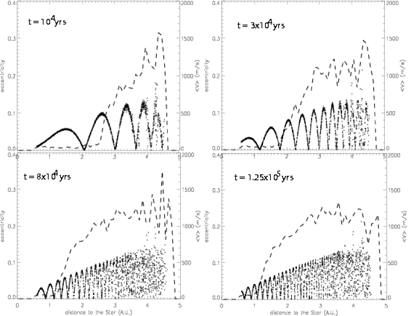
Figure 1: Evolution of a test particle population perturbed by a stellar companion with $m_{b}=0.25$, $a_{b}=20\,$AU and $e_{b}=0.3$. The dotted line represents the distribution of average encounter velocities within the system.

Our code is an updated version of a program initially developed for the study of planetesimal systems perturbed by a giant planet (e.g. Thébault et al., 2002) and recently used for the study of the $\gamma$ Cephei system (TH04). Let us here briefly outline that it deterministically follows the dynamical evolution of a population of massless test particles and that it has a close encounter search algorithm which enables tracking of all mutual encounters as well as accurate estimations of relative velocities at impact. Fig.1 shows a typical outcome for such a numerical run. The dynamical behaviour of the test particle system is dominated by eccentricity oscillations forced by the companion star. Once they begin to develop, the amplitude of these oscillations is almost constant with time and increases with proximity to the companion (i.e. in the outer regions). The frequencies of these oscillations do also increase with proximity to the companion but they do not remain constant and continuously increase with time. It is important to notice that, at least in the beginning, these large eccentricity oscillations do not lead to high encounter velocities because of the strong phasing between neighboring orbits. As times goes by, however, these oscillations get narrower and narrower, so that at some point the phasing can no longer prevent orbit crossing. This leads to a sudden increase of encounter velocities which may reach very high values, typically of the order of $10^{3}$m.s^-1. These values are high enough to prevent the accretion of any kilometre–sized planetesimal. As a consequence, the planetesimal accretion should be stopped in the orbit-crossing region, provided that no bigger object had the time to form before the orbital-crossing occurs. The transition between non orbit-crossing and orbit-crossing regions is very sharp, and one might consider that it occurs at one given semi-major axis $a_{cross}$. Notice that $a_{cross}$ progresses inward, so that the region of low $\Delta v$ gets narrower and narrower with time.

2.2 Analytical derivation

In order to avoid performing a tremendous amount of numerical runs exploring the full space of free parameters, we examine the possibility to get a reasonably accurate analytical formula giving the value of $a_{cross}$. Since we intend to study how accretion around a solar type primary star is affected by the companion’s perturbations, we chose a system of units related to the primary star. All masses are thus renormalized to the mass of the primary ($1\,M_{\odot}$), all distances to 1 AU and all times to 1 yr, i.e. the orbital period at 1 AU from the primary.

2.2.1 Revised expression for the secular approximation

The usual way to analytically describe perturbations triggered by a companion is to use the simplified secular perturbation theory equations for the eccentricity and longitude of periastron (e.g. Heppenheimer, 1978; Whitmire et al., 1998):

$$e=\frac{5}{2}\,\frac{a}{a_{b}}\,\frac{e_{b}}{1-e_{b}^{2}}|\sin\left(\frac{u}{2}t\right)|=e_{max}\,|\sin\left(\frac{u}{2}t\right)|$$ (1)

$$\tan(\varpi t)=-\frac{\sin ut}{1-\cos ut},$$ (2)

where

$$u=\frac{3}{2}\pi\frac{1}{\left(1-e_{b}^{2}\right)^{3/2}}m_{b}\frac{a^{3/2}}{a_{b}^{3}}.$$ (3)

Equation 1 gives a reasonably accurate estimation of the amplitude of the eccentricity estimations, the relative error being always smaller than $10\%$ for the set of parameters explored hereafter. However, due to the low order of its expansion, the expression for the frequency $u$ of these oscillations is a poor match to the ones numerically obtained, and differences can be as large as $70\%$. In order to empirically derive a more accurate prescription for $u$, we performed several numerical test runs and get the revised expression

$$u=\frac{3}{2}\pi\frac{1}{\left(1-e_{b}^{2}\right)^{3/2}}m_{b}\frac{a^{3/2}}{a_{b}^{3}}\,\left[1+32\frac{m_{b}}{\left(1-e_{b}^{2}\right)^{3}}\left(\frac{a}{a_{b}}\right)^{2}\right].$$ (4)

Equation 4 proved to be accurate within $5\%$ for the range of parameters here explored.

2.2.2 Orbital crossing location

Directly applying the classical orbital crossing criterion (e.g. Equ.6 of Whitmire et al., 1998) to Equs.1 and 2 results in an expression too complex to derive an analytical solution for $a_{cross}$. However, we empirically observed from our test runs that orbital crossing first occurs, within a given e-oscillation “wave”, when particles of high eccentricity within this wave are able to cross the orbit of particles at the “node” (i.e. e$\simeq 0$) of the wave. Furthermore, this crossing of the e=0 orbit occurs at almost the same time for all particles within one given wave. This crossing criterion might be written as

$$(a_{0}+\Delta a)\left(1-e_{(a_{0}+\Delta a)}\right)=a_{0}\Longleftrightarrow(a_{0}+\Delta a)\,e_{(a_{0}+\Delta a)}=\Delta a,$$ (5)

where $a_{0}$ is the semi-major axis of particles with $e=0$. If we restrict ourselves to the region where the width of an e-oscillation is always much smaller than its distance to the star (i.e. $\Delta a/a_{0}<<1$), then

$$a_{0}\,e_{(a_{0}+\Delta a)}\simeq\Delta a\Longrightarrow a_{0}\left(\frac{\partial e}{\partial a}\right)_{(a_{0})}\simeq 1.$$ (6)

Rewriting Equ.1 in the form $e_{max}\,sin(\theta_{(a)})$, it follows that

$$\left(\frac{\partial e}{\partial a}\right)_{(a_{0})}=e_{max}\left(\frac{\partial\theta}{\partial a}\right)_{(a_{0})}cos(\theta_{(a_{0})})=e_{max}\left(\frac{\partial\theta}{\partial a}\right)_{(a_{0})}\simeq\,\frac{\pi}{2}\frac{e_{max}}{\Delta a_{m}},$$ (7)

where $e_{max}$ is the maximum value of the oscillation wave (given by Equ.1) reached for $a=a_{(e_{max})}$, and $\Delta a_{m}=a_{(e_{max})}-a_{0}$ is such that

$$\frac{u_{(a_{0}+\Delta a_{m})}}{2}t-\frac{u_{(a_{0})}}{2}t=\frac{\pi}{2}\,\,\,\Longrightarrow\,\,\,{\Delta a_{m}}\frac{\partial u}{\partial a}=\frac{\pi}{t}.$$ (8)

Equation 4 then gives

$$\Delta a_{m}=\frac{2\pi}{3K}\frac{1}{a^{1/2}\left[1+\frac{224}{3}\frac{m_{b}}{\left(1-e_{b}^{2}\right)^{3}}\left(\frac{a}{a_{b}}\right)^{2}\right]}\,t^{-1},$$ (9)

where

$$K=\frac{3}{2}\pi\frac{1}{\left(1-e_{b}^{2}\right)^{3/2}}m_{b}\frac{1}{a_{b}^{3}}.$$ (10)

Putting Equ.1, Equ.7 and Equ.9 into Equ.6 gives

$$C_{1}a^{1/2}\left[\left(\frac{a}{a_{b}}\right)^{2}+C_{2}\left(\frac{a}{a_{b}}\right)^{4}\right]=\frac{1}{t},$$ (11)

where

$$C_{1}=\frac{45\pi}{16}\frac{e_{b}}{\left(1-e_{b}^{2}\right)^{5/2}}m_{b}\frac{1}{a_{b}^{2}}\,\,\,;C_{2}=\frac{224}{3}\frac{m_{b}}{\left(1-e_{b}^{2}\right)^{3}}.$$ (12)

Equation 11 is easily numerically solved and gives the value of the orbital crossing location $a_{cross}$ for any given set of parameters. The validity of Equ.11 has been checked by comparing its solution to numerically obtained estimates for extreme values of the free parameters of the problem ($a_{b}$, $m_{b}$, $e_{b}$). As Fig.2 clearly shows, there is always less than a $10\%$ relative error between the analytical estimate and the numerical values.

2.2.3 Relative velocities

Another important parameter is the average values of relative velocities $\langle\Delta v\rangle$ in the orbital crossing region beyond $a_{cross}$. From our series of test numerical runs, we have derived the simplified empirical relation

$$\langle\Delta v\rangle_{(a)}\simeq 0.5\,e_{max(a)}\,v_{kep(a)},$$ (13)

which proved to be of reasonable accuracy, i.e. less than 10% relative error. Note that this formula gives a value which is smaller, by roughly a factor 2, than the standard formulae giving average encounter velocities for completely randomized orbits $\langle\Delta v\rangle=(5/4)^{1/2}\,e\,v_{kep}$ (e.g. Equ.17 of Lissauer & Stewart, 1993). The main reason for this is that, despite orbital crossing, orbits are not fully randomized. A direct consequence of Equ.13 is that $\langle\Delta v\rangle$ has the same parameter dependency as $e$ (it is in particular independent of the companion mass $m_{b}$).

2.2.4 Parameter space exploration

We explore Equ.11 for a wide range of the companion’s orbital parameters and mass in order to map the region of parameter space allowing or preventing accretion at a given distance of the primary star. We consider as reference values for $a_{b}$, $e_{b}$ and $m_{b}$, the median values derived from Duquennoy and Mayor (1991) for their sample of G star binaries, i.e. $a_{b}\simeq 36\,$AU, $e_{b}\simeq 0.5$ and $m_{b}\simeq 0.5$. These parameters are then individually explored (Figs.3, 4 and 5). We focus here on the case of planets in the habitable zone and thus take 1 AU as a reference region of interest for the orbital crossing location.

One additional crucial parameter is the time $t_{cr}$ at which orbital crossing occurs. We will here pay particular attention to values between $5\times 10^{3}$ and $10^{5}$ years, i.e. a conservative range for typical runaway growth timescales. Figure 5 clearly illustrates the time dependency, showing a power law dependency between $t_{cr}$ and $a_{b}$ for $t_{cr}$ greater than a few thousand years. By thoroughly exploring the influence of all parameters on $t_{cr}$, we were able to derive the following empirical law, valid in the $a_{b}>10\,$AU and $0.05<e_{b}<0.8$ parameter range:

$$t_{cr}=\\ 6.98\times 10^{2}\frac{\left(1-e_{b}^{2}\right)^{3}}{e_{b}}\left(\frac{m_{b}}{1M_{\odot}}\right)^{-1.1}\left(\frac{a_{b}}{10\rm{AU}}\right)^{4.3}\left(\frac{a_{cross}}{1\rm{AU}}\right)^{-2.8}\rm{yrs}.$$ (14)

This gives in turn the location of $a_{cross}$ as a function of time and companion star parameters:

$$a_{cross}=0.37\frac{\left(1-e_{b}^{2}\right)^{1.07}}{e_{b}^{0.36}}\left(\frac{m_{b}}{1M_{\odot}}\right)^{-0.39}\left(\frac{a_{b}}{10\rm{AU}}\right)^{1.53}\left(\frac{t}{10^{4}yr}\right)^{-0.36}\,\rm{AU}\,.$$ (15)

This formulae, contrary to Equ.11, has been purely empirically obtained instead of analytically derived. As for Equ.11, we have checked its validity by comparison with a set of numerical tests exploring all extreme values for the parameters here explored. These comparisons showed that the value given by Equ.15 was always within a satisfying $10\%$ of the numerical result.

The corresponding expressions for the critical values of the companion’s semi-major axis and mass (the expression for $e_{b.cr}$ is more complicated and has to be numerically solved) as a function of $a_{cross}$ and time are then easely derived and read

$$a_{b.cr}=18.1\frac{e_{b}^{0.23}}{\left(1-e_{b}^{2}\right)^{0.69}}\left(\frac{m_{b}}{1M_{\odot}}\right)^{0.26}\left(\frac{a_{cross}}{1\rm{AU}}\right)^{0.65}\left(\frac{t}{10^{4}yr}\right)^{0.23}\,\rm{AU}$$ (16)

$$m_{b.cr}=8.95\times 10^{-2}\frac{\left(1-e_{b}^{2}\right)^{2.72}}{e_{b}^{0.91}}\left(\frac{a_{b}}{10\rm{AU}}\right)^{3.90}\left(\frac{a_{cross}}{1\rm{AU}}\right)^{-2.54}\left(\frac{t}{10^{4}yr}\right)^{-0.91}\,M_{\odot}.$$ (17)

3 EFFECT OF GAS DRAG

The results displayed in the previous section have been obtained for a simplified system where gravitational perturbing effects are the only forces acting on the planetesimal population. In the current standard planetary formation scenario however, the initial stages of planetesimal accretion are believed to take place in the presence of significant amounts of primordial gas. Gas drag affects planetesimal orbits by partially damping their eccentricity as well as forcing periastron alignment among bodies of the same size (e.g. Marzari & Scholl, 1998), thus cancelling the secular orbital oscillations induced by the perturber. These two effects might have drastic consequences on the onset of orbital crossing and on the values of impact velocities. In his earlier study, Whitmire et al. (1998) claimed the neglect of gas drag to be justified for bodies of size $\geq\,$10km. However, this argument might not hold for 2 reasons: 1) It is not clear if the initial planetesimal sizes were $\geq\,$10km (simply because it is not clear what this initial size actually is), and smaller objects should be more significantly affected by gas drag (this force being $\propto 1/R$). 2) Even for large planetesimals, the neglect of gas drag for $\geq\,$10km objects is a result that holds only for unperturbed planetesimal populations with low eccentricities. In the present case, we are dealing with high $e$ orbits for which gaseous friction is more effective, since gaseous eccentricity damping is expected to be $\propto e^{2}$ (Adachi et al., 1976). A study of planetesimal accretion in binary systems can thus probably not dispense from addressing the crucial issue of gas drag effects. The non-conservative characteristics of gaseous friction as well as the number of additional free parameters it introduces, i.e. gas density and distribution, planetesimal absolute and relative physical sizes, etc.., renders a semi-empirical analytical analysis in the spirit of the one presented in the previous section almost impossible. We have here to rely on numerical simulations. Numerical studies of gaseous friction have been undertaken by the present team in several previous works for specific perturbed systems, e.g. Marzari & Scholl (1998, 2000); Thébault et al. (2002) and TH04 for the specific case of the $\gamma$ Cephei binary system. The aim of the present study is to generalize these previous studies to the general case of any binary system.

3.1 Modeling

The numerical code is the same as the one used in Thébault et al. (2002) and TH04. We follow Weidenschilling & Davis (1985) and model the gas force as

$$\vec{F} = -Kv\vec{v},$$ (18)

where $\vec{F}$ is the force per unit mass, $\vec{v}$ the velocity of the planetesimal with respect to the gas, $v$ the velocity modulus, and $K$ is the drag parameter. It is a function of the physical parameter of the system and is defined as:

$$K = \frac{3\rho_{\rm g}C_{d}}{8\rho_{{\rm pl}}R},$$ (19)

where $\rho_{\rm g}$ is the gas density, $\rho_{{\rm pl}}$ and $R$ the planetesimal density and radius, respectively. $C_{d}$ is a dimensionless coefficient related to the shape of the body ($\simeq 0.4$ for spherical bodies).

Exploring the gas drag density profile as a free parameter would be too CPU time consuming and we shall restrict ourselves to one $\rho_{\rm g}$ distribution. We assume the standard Minimum Mass Solar Nebula (MMSN) of Hayashi (1981), with $\rho_{\rm g}=\rho_{\rm g0}(a/1AU)^{-2.75}$ and $\rho_{\rm g0}=1.4\times 10^{-9}$g.cm^-3. We take a typical value $\rho_{\rm pl}=3\,$g.cm^-3. Since the initial sizes of accreting planetesimals are not very well constrained, we shall consider two types of detailed simulations, i.e. one for a typical “small planetesimals” case, where $1<R<10\,$km, and one for a typical “big planetesimals” case with $10<R<50\,$km. For each case, the main outputs are the values of encounter velocities $\Delta v_{(R1,R2)}$ for all possible target-projectile pairs of sizes $R_{1}$ and $R_{2}$.

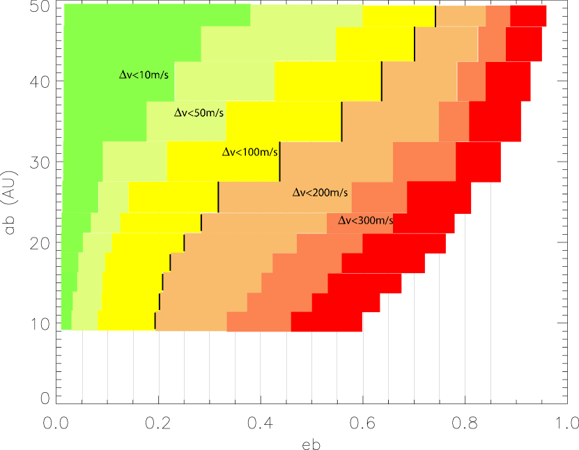
Figure 8: Encounter velocities averaged, over the time interval $0<t<2\times 10^{4}$yrs, between $R_{1}=2.5$ and $R_{2}=5\,$km bodies at 1 AU from the primary star, for different values of the companion star semi-major axis and eccentricity. The short black vertical segments mark the limit beyond which $<\Delta v_{(R1,R2)}>$ values correspond to eroding impacts for all tested collision outcome prescriptions.

To interpret these results in terms of accreting or eroding impacts, the obtained $\Delta v_{(R1,R2)}$ values have to be compared to reference semiempirical models of collisional outcomes. The core assumption for these models are the prescriptions for cratering excavation factors and the disruption threshold parameter $Q_{*}$. Several different such prescriptions, based on laboratory experiments and/or energy scaling considerations, are currently available. One has however to remain careful since many of these prescriptions are far from agreeing with each other and often predict very different physical outcomes for a given set of $R_{1}$, $R_{2}$ and $\Delta v_{(R1,R2)}$ parameters (a striking illustration of this can be found in Fig.8 of Benz & Asphaug, 1999, where values of $Q_{*}$ from different authors are compared). We shall here analyze our $\Delta v_{(R1,R2)}$ values using the statistical model of Thébault et al. (2003), a detailed numerical tool developed for the study of collisional cascades in extrasolar disks, which can accommodate for different $Q_{*}$ and cratering excavation coefficient prescriptions. We here explore 3 different $Q_{*}$ prescriptions, i.e. Marzari et al. (1995), Holsapple (1994) and Benz & Asphaug (1999) and two “soft” and “hard material” cases for the cratering excavation coefficient. We remain as careful as possible and shall only consider that impacts are preferentially accreting or eroding when all tested prescriptions agree, and do not derive definitive conclusions for the intermediate “limbo” region where different outcomes are obtained depending on the assumed collisional formalism.

To get statistically significant results all runs include $N=10^{4}$ test particles.

3.2 Typical behaviour

Let us first present results obtained for two representative “pedagogical” companion configurations: 1) $a_{b}=10\,$AU, $e_{b}=0.3$, $m_{b}=0.5$, a highly perturbed case for which Equ.14 predicts fast orbital crossing, at 1 AU, under pure secular perturbations 2) $a_{b}=20\,$AU, $e_{b}=0.4$, $m_{b}=0.5$, a less perturbed case with no predicted orbital crossing occurring before $5\times 10^{4}$yrs. For these two illustrative examples, we display the results in full matrices of average encounter velocities $\Delta v_{(R1,R2)}$ for all impacting pairs of sizes $R_{1}$ and $R_{2}$ in the “small” and “big” planetesimals runs. Presented $\Delta v$ values are averaged over a typical runaway growth time interval $0<t<2\times 10^{4}$yrs, but no crucial time dependent information is lost, since in general $\Delta v_{(R1,R2)}$ values set in on timescales of only a few $10^{3}$yrs.

3.2.1 highly perturbed case: $a_{b}=10\,$AU, $e_{b}=0.3$, $m_{b}=0.5$

Fig.6 shows the typical dynamical evolution for two planetesimal populations of different sizes. The most obvious feature is the forced orbital alignment among equal-sized bodies. In the present example, it is strong enough to prevent any orbital crossing, within $2\times 10^{4}$years, for all equal-sized small planetesimals (Fig.7). For bigger objects in the $50$ km size range, orbital crossing occurs, at approximately the time predicted by the previous section’s set of equations, although for encounter velocities significantly smaller than in a gas free case. For bodies of different sizes however, results are almost the exact opposite. Indeed, orbital alignment strongly depends on planetesimal radius: smaller objects tend to align more quickly and towards periastron values located at $\simeq$ 270 degrees from that of the perturber $\varpi_{p}$, while bigger bodies need more time to align their orbits and do it towards periastron values closer to $\varpi-\varpi_{p}\simeq 360^{o}$ (a result already identified by Marzari & Scholl, 1998). This is clearly illustrated in Fig.6, with 1km objects on fully phased orbits after $3\times 10^{3}\,$yrs while 5km bodies haven’t reached complete alignment yet, especially in the outer regions where residual secular oscillations are still visible. The consequence of this differential periastron alignment is a fast and significant increase of encounter velocities between these 2 populations (Fig.7). The full $\Delta v_{(R1,R2)}$ matrixes of Tabs.1 and 2 show that this result holds for all sizes: differential phasing always results in $\Delta v$ increase as soon as $R_{1}\neq R_{2}$. In contrast, the $\Delta v$ damping effect between equal-sized objects appears as only a marginal feature, especially in the 1-10km range. Indeed, if as a first approximation we parameterize the collisional efficiency of a $\Delta v_{(R1,R2)}$ impact by the amount of kinetic energy $Ec_{(R1,R2)}$ delivered to the target $R_{2}$ by an $R_{1}$ ($<R_{2}$) impactor, then an exploration of the values displayed in Tab.1 shows that $Ec_{(R1,R2)}$ always exceeds $Ec_{(R2,R2)}$ for $R_{2}\leq 10\,$km. As a matter of fact, for most impacting pairs in this size range the delivered kinetic energy peaks at roughly $R_{1}\simeq 1/2R_{2}$. The crucial result is in any case that, for almost all $R_{1}\neq R_{2}$ impacts of the small planetesimals run, encounter velocities exceed by far the limit for accretion and the system should clearly undergo erosion (Tab.1).

Things are less simple in the big planetesimals run. The only low velocity collisions are those between equal-sized bodies smaller than 20 km. For bigger objects gas drag can no longer prevent orbital crossing and the corresponding velocity increase. For objects of different sizes, differential orbital phasing has the same velocity increase effect as in the small planetesimal case; although it is a bit more complicated here, where the obtained $\Delta v_{(R1,R2)}$ is often a combination of an orbital crossing and of a differential phasing term (for which the delivered kinetic energy $Ec_{(R1,R2)}$ peaks for $R_{1}/R_{2}$ values close to $\simeq 1/3$). Note however that encounter velocities never reach values for which we might be sure that erosion dominates over accretion. $\Delta v_{(R1,R2)}$ values are here in the “limbo” range where empirical collisional outcome models disagree on the net accretion vs. erosion balance (Tab.2).

3.2.2 moderately perturbed case: $a_{b}=20\,$AU, $e_{b}=0.4$, $m_{b}=0.5$

This case should in principle be radically different from the previous one, as Equ.14 predicts that no orbital crossing should occur within the timeframe of the simulation. For the small planetesimals run however, results are remarkably similar to those of the $a_{b}=10\,$AU, $e_{b}=0.3$, $m_{b}=0.5$ case: differential orbital phasing induced by gas drag restricts low velocity impacts to a narrow $R_{1}\simeq R_{2}$ diagonal and $\Delta v_{(R1,R2)}$ are clearly in the eroding regime for a large majority of impacting pairs (Tab.3). As in the previous example, $Ec_{(R1,R2)}$ always exceeds $Ec_{(R2,R2)}$ and the delivered kinetic energy also peaks for $R_{1}\simeq 1/2R_{2}$. Differences are nevertheless observed for the $10<R<50\,$km run, where although velocity increase is observed for almost all $R_{1}\neq R_{2}$ pairs, its amplitude remains more limited than for the previous highly perturbed case. The main reason for this difference is that here we have only the gas drag induced velocity increase but no contribution due to secular orbital crossing. This is why $\Delta v_{(R1,R2)}$ remain relatively small for the bigger, less affected by gas drag, objects (in the $R\gtrsim 25$km range). As a consequence, most of mutual collisions in the “big planetesimals” run turn out to result in net accretion (Tab.4).

3.2.3 radial drift

In addition to orbital alignment and eccentricity damping, it is well known that gas drag also forces inward drift of planetesimals (e.g. Thébault et al., 2004). This drift could in principle also be the source of a $\Delta V$ increase: the radial drift being size dependent it might bring to the same location objects ”carrying” with them different periastron values depending on their region of origin. However, this effect appears to be negligible here. Indeed, the average inward drift of a 1 km object (the smallest size considered here) starting at 1 AU is $\simeq 1.6\times 10^{-5}$AU.yr^-1 for the highly perturbed case. This means that it has drifted by less than 0.05 AU by the time complete periastron alignment is reached, i.e. $3.\times 10^{3}\,$years. From Fig.6 it is easy to see that the difference in periastron between 1.05 and 1 AU is small compared to the $local$ periastron difference, at 1 AU, between a 1 km and a 5 km object. In other words, local periastron phasing effects are much more efficient (i.e. fast) than periastron ”transport” from one place to another, even in the extreme case where objects would carry their periastron without modifications from one place to another. Another proof of the insignificance of this effect is that if it was efficient then it should also affect the $\Delta V$ distribution between $equal$–sized objects, since even same–size objects originating from different regions have different drift rates and could thus be brought together. But, as already mentioned, no $\Delta V$ increase is observed in our simulations for equal–sized planetesimals (except for the non-gas drag induced effects on bigger planetesimals).

3.3 $a_{b}$ and $e_{b}$ parameter exploration

For obvious computing time constraints, it is impossible to thoroughly explore all companion orbital parameters with simulations as detailed as those presented in the previous section. We shall narrow our exploration range by fixing the companion’s mass to a typical value $m_{b}=0.5$ that of the primary and explore $a_{b}$ and $e_{b}$ as free parameters in the $10<a_{b}<50$AU and $0.05<e_{b}<0.9$ ranges. A total number of 126 runs have been performed. As already mentioned, we perform, for each companion configuration, 2 runs, for a “small” and a “big” planetesimals case respectively. For sake of readability of the results, we display the obtained $\Delta v_{(R1,R2)}$ values for specific $R_{1}$ and $R_{2}$ values corresponding to a typical pair of impacting bodies for each case. We take $R_{1}=2.5$ and $R_{2}=5\,$km as representative values for the small planetesimals run since, for most of the $e_{b}$ and $a_{b}$ range explored here, simulations confirm the results obtained for the previous specific examples, i.e. that bodies delivering the maximum kinetic energy to a $R_{2}$ target are roughly those of size $R_{1}\simeq 1/2R_{2}$. For the bigger planetesimals, the delivered kinetic energy peaks for somewhat smaller $R_{1}/R_{2}$ ratios and we consider $R_{1}=15$ and $R_{2}=50\,$km as typical example values. As in the previous section, we display encounter velocities averaged over $0<t<2\times 10^{4}$yrs.

3.3.1 small planetesimals case

A first important result is that we never observe velocity increase between equal-sized small planetesimals, i.e. gas drag orbital alignment prevents orbital crossing from occurring for all the ($a_{b},e_{b}$) space explored here. However, we observe a generalization of the previous section’s result, i.e. a dramatic $\Delta v_{(R1,R2)}$ increase as soon as $R_{1}\neq R_{2}$. This is clearly illustrated in Fig.8 for a typical $R_{1}=2.5$ and $R_{2}=5\,$km pair. We can schematically divide this graph into 3 regions:

• The region where encounter velocities remain at their initial low values ($\Delta v\leq 10\,$m.s^-1). This fully undisturbed region is confined to a narrow strip close to $e_{b}=0$ except for large $a_{b}>40$AU values. Its extent is very limited when compared to the corresponding undisturbed region in the gas free case, i.e. the one given by the limit for orbital crossing at $t\simeq 2\times 10^{4}$yrs (see Fig.3)

• The $10\leq\Delta v\leq 100\,$m.s^-1 region. Here, encounter velocities begin to be significantly increased by differential orbital phasing. The net collisional outcome remains however uncertain, since we are in the “limbo” range where the balance between accretion and erosion depends on the assumed collisional outcome prescription. This intermediate zone covers a large fraction of the ($a_{b},e_{b}$) space. Interestingly, its borders are almost independent of $e_{b}$ for $a_{b}<20$AU.

• The $\Delta v\geq 100\,$m.s^-1 region where encounter velocities are increased to values always exceeding the net erosion threshold. This zone still covers an area much more extended than that of the orbital-crossing region of the gas free case. This is particularly true for companion semi-major axis comprised between 20 and 40 AU.

3.3.2 large planetesimals case

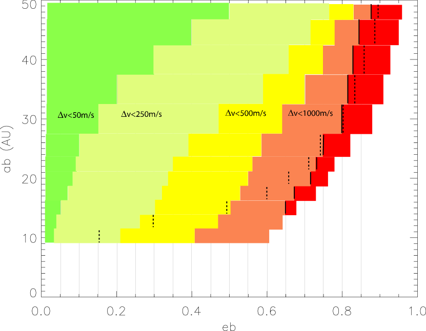
Figure 9: Same as Fig.8, but for $R_{1}=15$ and $R_{2}=50\,$km bodies. The short black vertical segments mark the limit beyond which $<\Delta v_{(R1,R2)}>$ values correspond to eroding impacts for all tested collision outcome prescriptions. The short dashed vertical segments mark the position beyond which orbital crossing occurs for 50 km bodies.

The situation is slightly more complex when considering a population of larger objects. An important point is that gas drag is less efficient and no longer able to systematically prevent orbital crossing, especially for the biggest bodies (Fig.9). As an example, for the 50 km objects considered in Fig.9, simulations show that orbital crossing always occurs as predicted if $t_{cr}\leq 10^{4}$yrs (the positions of the limit for orbital crossing approximately match that of the $t_{cr}=10^{4}\,$yrs line in Fig.3) but is prevented if it requires longer timescales (in this case, gas drag has more time to affect the bodies orbital evolution). It is worth noticing that gas drag can never delay orbital crossing: either it prevents it or it does not, and in this case crossing occurs at the time predicted by Equ.3. The only difference lies in the values of encounter velocities after orbital crossing, which are always significantly lower than in the gas free case. They remain however always high enough, i.e. $\geq 350$m.s^-1 for 50km bodies, to correspond to eroding impacts. For $R_{1}\neq R_{2}$ bodies, differential orbital phasing increases relative velocities to values generally higher than for the small planetesimal case. Nevertheless, the consequences of these high $\Delta v$ are less radical in terms of accretion inhibition efficiency. If we divide the $(a_{b},e_{b})$ parameter space in a similar way as for the previous case, then we see that the region of fully unperturbed encounters ($\Delta v\leq 50$m.s^-1) is slightly more extended. More interesting is maybe the extent of the $50\leq\Delta v\leq 250$m.s^-1 region, in which accretion still prevails despite of the increased encounter velocities, and of the “limbo” zone $250\leq\Delta v\leq 1000$m.s^-1 with uncertain accretion vs. erosion balance. Those 2 combined areas fill up most of the parameter space, leaving only a small fraction for without–doubt eroding $\Delta v\geq 1000$m.s^-1 impacts. Note also that these eroding impacts almost always occur beyond the orbital crossing limit for equal-sized 50 km bodies.

4 DISCUSSION

Comparing Figs.8 and 9 to Fig.3 for pure gravitational perturbing effects clearly shows to what extent gas drag affects the encounter velocity evolution. On one hand, orbital alignment and eccentricity damping due to gas friction tends to prevent orbital crossing and even if it occurs, $\Delta v$ are lower than in the gas free case. But on the other hand, gas drag introduces an additional source of velocity increase due to differential orbital alignment for bodies of different sizes. This additional term proves to be very efficient, leading to a $\Delta v$ increase for any departure from the exact $R_{1}=R_{2}$ condition. Furthermore, this increase is significant in a much larger region of the ($e_{b}$,$a_{b}$) phase space than that delimited by the orbital-crossing limit in the gas free case (Figs.8 and 9). The global balance between these impacts for which gas drag tends to slow down or prevent accretion, and impacts where gas drag favours mutual growth, i.e. those with 2 bodies of comparable sizes, depends of course on the planetesimal initial size distribution, and in particular the spread in planetesimal radius, a parameter which is not very well constrained in current planetary formation scenarios. This important issue is clearly beyond the scope of the present study. However, it is important to notice that large differential phasing $\Delta v$ terms arise for any small departure from the exact $R_{1}=R_{2}$ condition. As an example, for most tested cases a relative $\Delta R/R$ displacement of only 10% from the equal-size configuration results in a factor 2 (at least) increase in encounter velocities. As a consequence, the low $\Delta v$ between equal–sized objects appears as a relatively marginal result. It is likely that in a realistic planetesimal population, with a statistical spread in object sizes, the dominant effect of gas drag is the velocity increase due to differential orbital phasing.

To what extent does this velocity increase affect the accretional evolution of the system? The answer to this question depends mainly on the typical sizes within the “initial” planetesimal swarm. Should this initial population be made of small ($\leq 10$ km) objects, then gas drag would probably present a major threat to accretion, at least in the $a_{b}\leq 50\,$AU range explored here. Even taking our conservative criteria for fully eroding impacts, Fig.8 clearly shows that the fraction of accretion–inhibiting ($e_{b},a_{b}$) configurations is much higher than in the gas free case. As an example, for pure secular perturbations most configurations with $a_{b}\geq 15\,$AU are accretion friendly when $e_{b}\lesssim 0.7$, whereas for gas drag and 5 km planetesimals, in the same $a_{b}\geq 15\,$AU domain, the accretion/erosion frontier is approximately delimited by a $(a_{b}-4{\rm AU})-60\,e_{b}\simeq 0\,\,$ line. Furthermore, even if accretion is in principle possible in the “limbo” $10<\Delta v<100$m.s^-1 region of Fig.8, it can not be of a standard runaway type. Indeed, runaway growth can only develop when encounter velocities are significantly lower than the growing bodies escape velocity, increasing their geometrical cross section by a gravitational focusing factor proportional to $(v_{esc}/\Delta v)^{2}$ (e.g. Greenberg et al., 1978). Such a focusing factor would be made negligible by the encounter velocity increase in the “limbo” zone, where $\Delta v$ always exceed the escape velocity of a $\leq 10\,$km body. This leaves only a very limited ($e_{b},a_{b}$) region (the “green” area of Fig.8) where standard runaway accretion can develop, i.e. where encounter velocities do not exceed the escape velocities of typical $R<10\,$ km bodies. For bigger $10<R<50\,$km objects, the situation is significantly different. Here, differential orbital phasing almost never increases $\Delta v$ to values high enough to correspond to eroding impacts for all tested collision prescriptions. For most cases, the limit for eroding impacts is actually given by the limit for orbital crossing, thus probably making the latter mechanism the decisive factor for accretion-inhibition. However, we are not back to a simple black-or-white alternative as in a gas free case. Indeed, in most of the cases below orbital crossing, $\Delta v_{R1\neq R2}$ are increased to values exceeding the escape velocity of a $50\,$km body. As already mentioned, this would prevent the onset of standard runaway growth by decreasing the gravitational focusing factor. The ($a_{b},e_{b}$) space for unperturbed runaway accretion is then restricted to a region only marginally more extended than in the small planetesimals case.

In the extended “limbo” regions of both big and small planetesimals runs, a possible accretion growth mode would be the “type II” runaway accretion identified by Kortenkamp et al. (2001) in the context of giant planets’ perturbations on a swarm of planetesimals. Like in the present “limbo” zones, type II accretion is characterized by initial encounter velocities increased by differential gas–drag orbital phasing to values exceeding the biggest objects’ escape velocities, but without erosion overcoming accretion. The first step of this scenario is “orderly” growth (Safronov, 1969) characterized by a slow and progressive growth of all planetesimals. Growth later switches to runaway when the biggest bodies reach a size large enough for gravitational focusing to become significant again. For the specific case studied by Kortenkamp et al. (2001), this size was approximately that of Ceres. This turn–off size should of course vary with the $m_{b},a_{b},e_{b}$ parameters of the perturber, but in a first approximation Fig.9 shows that the escape velocity of a Ceres–type object of radius $\simeq 500\,$km would indeed exceed $\Delta v$ values in most of the parameter space “left of” the orbital crossing limit.

5 LIMITATION TO THIS APPROACH AND PERSPECTIVES

5.1 Initial conditions

One assumption made in our analytical derivations and numerical simulations is to start from an initial system of objects on circular orbits with very low relative velocities. As already mentioned, this is implicitly equivalent to assuming that the spread $\Delta t_{0}$ in the timescales for the formation of kilometre-sized planetesimal is negligible compared to the characteristic timescales for secular perturbations and planetesimal accretion. As discussed in section 2, the validity of this assumption is directly linked to the difficult problem of the mechanism for planetesimal formation. This mechanism is still poorly understood and we believe our initial conditions to be relatively reasonable within the frame of the current dust-to-planetesimals formation process knowledge.

One has nevertheless to be aware of the possible effects $\Delta t_{0}$ might have on the presented results. For the pure gravitational case, our assumption of initial very small relative velocities breaks down if $\Delta t_{0}$ is no longer negligible compared to $1/u$. In this case the first formed planetesimals have the time to reach high eccentricities before the later ones decouple from the gas, leading to an initial high free $\Delta v$ component which cannot be damped by later secular effects. Equ.4 shows that the typical limiting values for $\Delta t_{0}$ are in the $\simeq 10^{3}$–$10^{4}\,$years range depending on the companion’s orbital parameter, in particular $a_{b}$.

In the gas drag runs, the effect of an initial $\Delta t_{0}$ is less critical, since gas friction tends to progressively damp any initial orbital differences toward the same equilibrium value. This is clearly illustrated in the example displayed in Fig.10, where we artificially introduce an initial $\Delta t_{0}$ by allowing initial eccentricities to vary between 0 and the value they would reach at the end of the gas drag induced phasing (thus implicitly assuming that some objects appeared earlier than others and had enough time to be affected by the coupled effect of secular perturbations and gas drag). As can be seen, the initial high $\Delta v_{R1,R2}$ values are progressively damped and after a transition period of less than $\simeq 10^{4}\,$years converge towards the same equilibrium values than those obtained when starting from circular orbits. The duration of this critical transition period is of course dependent of the companion star orbital parameters and of planetesimal sizes, and it might in some cases be long enough to significantly affect the accretion process. Possible effects of initial $\Delta t_{0}$ can thus not be ruled out within the frame of our present knowledge of the planetesimal formation process. It is however important to note that any initial $\Delta t_{0}$ would necessarily act in the direction of accretion $inhibition$ by adding an additional $\Delta v$ term. Our results might thus be considered as a lower limit for perturbing effects within binaries.

5.2 Gas friction modeling

Our gas drag model is a simplified one where the gas disk is assumed to be fully axisymmetric and follows a classical Hayashi (1981) power law distribution. It is however more than likely that in reality the gas disk should depart from this simplified view because it would also ”feel” the companion star’s perturbations. Several numerical studies have investigated the complex behaviour of gaseous disks in binary systems. They all show that pronounced spiral structures rapidly form within the disk (e.g. Artymowicz and Lubow, 1994; Savonije et al., 1994) and that gas streamlines exhibit radial velocities. To follow the dynamical behaviour of planetesimals in such non-axisymmetric gas profiles would require a study of the $coupled$ evolution of both gas and planetesimal populations, which would probably have to rely on hydro–code modeling of the gas in addition to N–body type models for the planetesimals. Such an all–encompassing gas$+$planetesimals modeling is clearly the next step in binary disk studies.

5.3 Do planetesimals really form?

One implicit assumption behind our simulations is of course that, as some point, kilometre-sized planetesimals $do$ form in the system. With our present understanding of the planet–formation–in–binaries problem, nothing allows us to be sure that this assumption is valid. The crucial problem of how dust sticking and/or dust settling and gravitational instabilities can proceed in a binary system remains yet to be investigated. Problems could also arise at even earlier stages. Nelson (2000) has for instance shown that, under certain conditions, thermal energy dissipation in gas disks for equal mass binaries could inhibit dust coagulation by raising temperatures above vaporization limit. But, as recognized by the author himself, these results are still preliminary, and a complete study of this problem, taking into account a broader range of physical parameters, has yet to be carried out.

6 SUMMARY

We explore the effect of gravitational perturbations of a stellar companion of semi–major axis $a_{b}\leq 50\,$AU on a planetesimal population orbiting the primary star, with particular focus on the 1 AU region. We concentrate on the relative velocity distribution, the key parameter for the evolution of a planetesimal population, which can only accrete each other if $\Delta v$ remain below a threshold value which depends on planetesimal sizes. We investigate the companion’s influence on this distribution for timescales comparable to that of the standard runaway growth scenario.

We first address the simplified pure gravitational problem. In this case, the companion stars triggers strong phased secular orbital oscillations which might eventually become so narrow that neighboring orbits cross, leading to abrupt encounter velocity increase. We derive a set of semi-analytical expressions to determine this orbital crossing location as a function of time. Assuming initial coapsidality for planetesimal orbits at 1AU from the primary, we find that for a large fraction of companion orbital parameter configurations, schematically for $a_{b}\geq 15\,$AU and $e_{b}\leq 0.6$–$0.7$, orbital crossing does not occur within typical runaway timescales of $\simeq 10^{4}\,$years. For the cases where orbital crossing occurs, however, impacts velocities reach values almost always too high to allow mutual accretion.

The inclusion of gas drag greatly complicates this black-or-white picture and leads to a large spectrum of impact velocities between planetesimals depending on their size and on the binary orbital parameters. In our numerical exploration we observe the well known effect of forced orbital alignment between equal-sized objects which prevents orbital crossing from occurring for most planetesimal sizes explored here. But this effect is balanced by the $\Delta v$ increase between objects of different sizes due to the strong size dependency of the gas drag induced orbital phasing. In fact, we find that this differential phasing term is so sensitive to any small departure from the exact equal–size case that it is likely to be the dominant effect in any ”real” planetesimal population with even a limited spread in planetesimal sizes. For a typical companion mass $m_{b}=0.5$ and for the range of semi-major axis here explored ($a_{b}\leq 50\,$AU) we find that ”standard” runaway accretion, where $\Delta v$ remain smaller than bodies’ typical escape velocities $v_{esc}$, is only possible for companion eccentricities close to 0. In the rest of the ($e_{b}$,$a_{b}$) parameter space, impact velocities always exceed $v_{esc}$ and might even exceed the threshold values $v_{ero}$ for which the net balance for collision outcomes is erosion instead of accretion. We can thus basically divide the ($e_{b}$,$a_{b}$) parameter space in 3 regions

• The domain where $\Delta v\leq v_{esc}$. Here we expect the companion’s perturbation to have a negligible influence on the accretion evolution of the system. This region is relatively narrow, for all planetesimal sizes explored, for $a_{b}\leq 40\,$AU.

• The region where $\Delta v$ exceeds the erosion threshold value for any realistic collision outcome prescriptions we tested. The extent of this region depends on the planetesimal sizes. It is relatively wide for “small” $\leq 10\,$km bodies, where this accretion inhibition mechanism is much more efficient than orbital crossing in the gas free case. For objects in the $\simeq 50\,$km size range, the $\Delta v\geq v_{ero}$ condition is met in a more limited ($e_{b}$,$a_{b}$) domain. Besides, it occurs mostly for configurations where secular orbital crossing occurs despite gas friction, so that the latter mechanism is probably the dominant one for inhibiting accretion of large objects.

• In between these 2 well defined domains, there is an intermediate region where accretion is possible despite $\Delta v$ values exceeding $v_{esc}$, or where the erosion vs. accretion net balance is uncertain, i.e. it depends on the assumed collisional outcome model. Here, a possible accretion evolution scenario could be the type II runaway growth identified by Kortenkamp et al. (2001), where accretion starts in a slow orderly way, and only later switches to runaway when larger planetesimals have formed.

.

Acknowledgements

The Authors wish to thank Eiichiro Kokubo and an anonymous referee for fruitful comments and suggestions that helped improve the paper a lot

Table 1: Average encounter velocities in m.s^-1, at 1 AU from the primary, within a population of “small” planetesimals $1<R<10\,$km for a gas drag simulation with the companion star parameters $m_{b}=0.5$, $a_{b}=10\,$AU and $e_{b}=0.3$. $\Delta v_{R1,R2}$ values are averaged over the time interval $0<t<2\times 10^{4}$yrs. Initial starting encounter velocities are such as $\Delta v_{0}\simeq 10$m.s.^-1. $\Delta v$ values in bold correspond to accreting impacts for all tested collision outcome prescriptions. Underlined values are those for which we obtain different accretion vs. erosion balance depending on the tested prescription. Values in classical roman characters correspond to cases for which all tested models agree on a net erosive outcome.

Sizes (km)	1	2	3	4	5	6	7	8	9	10
1	10	154	233	285	327	360	391	426	452	458
2	172	10	94	133	187	223	262	287	316	334
3	238	84	11	54	99	137	177	200	230	254
4	289	144	63	12	40	80	115	149	171	198
5	325	188	103	43	12	32	70	100	122	154
6	373	228	144	83	32	11	36	56	84	104
7	400	261	182	113	68	36	12	35	48	76
8	428	298	212	147	98	56	35	12	36	45
9	450	310	238	168	123	83	48	36	13	31
10	453	338	263	196	152	107	73	48	31	13

Table 2: Same as Table 1, but for a population of bigger planetesimals $10<R<50\,$km. Initial starting encounter velocities are such as $\Delta v_{0}\simeq 30$m.s.^-1

Size (km)	10	15	20	25	30	35	40	45	50
10	28	100	163	216	261	296	329	364	385
15	99	29	109	149	204	243	277	314	345
20	170	108	133	128	177	223	249	289	324
25	215	155	140	158	183	211	224	274	304
30	263	208	185	183	221	238	247	283	316
35	299	250	218	208	237	251	253	273	311
40	337	282	259	225	257	274	257	299	335
45	365	320	291	261	277	279	276	341	338
50	387	339	321	299	303	293	314	332	356

Table 3: Same as Table 1, i.e. “small” planetesimal population, but with companion star parameters $m_{b}=0.5$, $a_{b}=20\,$AU and $e_{b}=0.4$.

Sizes (km)	1	2	3	4	5	6	7	8	9	10
1	11	127	204	255	298	342	368	390	417	442
2	126	10	84	139	185	227	258	290	317	340
3	200	91	11	68	108	158	186	218	246	272
4	258	146	61	9	48	88	120	154	186	209
5	301	192	113	54	12	44	75	111	136	164
6	339	232	152	99	43	10	31	66	92	119
7	361	262	181	126	77	28	13	26	56	87
8	395	295	219	159	112	68	26	11	28	48
9	425	320	246	190	136	92	55	25	11	23
10	446	346	266	208	163	122	82	49	22	12

Table 4: Same as Table 3 but for the “big” planetesimal population.

Size (km)	10	15	20	25	30	35	40	45	50
10	26	95	154	198	231	265	292	312	335
15	92	27	73	115	148	179	210	234	268
20	157	75	32	51	88	125	146	170	208
25	197	111	54	29	48	74	101	121	145
30	235	149	90	47	28	40	63	87	101
35	266	184	117	75	42	30	37	56	73
40	290	208	145	97	65	40	32	36	53
45	308	226	167	120	86	59	37	31	33
50	341	272	207	144	104	77	56	38	35

Figure 2: Comparison between the analytical expression for orbital crossing location given by Equ.11 (lines) and values obtained for numerical test runs (crosses). The companion star has a semi-major axis $a_{b}=20\,$AU and 3 different eccentricities. Companion masses are given in solar mass units.

Figure 3: Value of the minimum companion semi-major axis, $a_{b.cr1}$, leading to orbital crossing of planetesimals at 1 AU, for different values of the crossing time $t_{cr}$, as a function of the companion eccentricity. The companion’s mass is fixed, with $m_{b}=0.5$. The dotted lines represent constant values of $\langle\Delta v\rangle$ at orbital crossing, as given by Equ.13

Figure 4: Value of $a_{b.cr1}$ (same definition as in Fig.3), for the same 4 values of $t_{cr}$ as in Fig.3, as a function of the companion mass. The companion’s eccentricity is fixed, with $e_{b}=0.5$.

Figure 5: Time for orbital crossing at 1 AU, as a function of the companion semi–major axis, for 4 different values of $e_{b}$, and $m_{b}=0.5$

Figure 6: Example gas drag run. Snapshots, at $t=3\times 10^{3}$yrs, of the ($e,a$) and ($\varpi-\varpi_{b},a$) distributions for 2 planetesimal populations of size $R_{1}=1\,$km and $R_{2}=5\,$km. $\varpi-\varpi_{b}$ is the difference, in angular degrees, between the particles and the companion star’s longitude of periastron. The companion star orbital parameters are: $a_{b}=10\,$AU, $e_{b}=0.3$, $m_{b}=0.5$

Figure 7: Gas drag run. Temporal evolution of mutual encounter velocities $\Delta v_{(R1,R2)}$ for different target-projectile pairs $R_{1}$ and $R_{2}$. The vertical line shows the moment where orbital crossing should occur, due to pure secular perturbations, according to Equ.14. Companion star orbital parameters: $a_{b}=10\,$AU, $e_{b}=0.3$, $m_{b}=0.5$

Figure 10: Average encounter velocities, at 1 AU from the primary, between planetesimals of different sizes for 2 different initial conditions: a) circular orbits b) initial eccentricities randomly distributed between 0 and the equilibrium phased value. The companion’s orbital parameter are $a_{b}=30\,$AU, $e_{b}=0.4$, $m_{b}=0.5$

References

- Adachi et al. (1976) Adachi, I., Hayashi, C., Nakagawa, K., 1976, The gas drag effect on the elliptical motion of a solid body in the primordial solar nebula, Prog. Theor. Phys., 56, 1756
- Artymowicz and Lubow (1994) Artymowicz, P., Lubow, Stephen H., 1994, Dynamics of binary-disk interaction. 1: Resonances and disk gap sizes, ApJ, 421, 651
- Barge & Pellat (1993) Barge, P., Pellat, R., 1993, Mass spectrum and velocity dispersions during planetesimal accumulation, Icarus, 104, 79
- Benz & Asphaug (1999) Benz, W., Asphaug, E., 1999, Catastrophic Disruptions Revisited, Icarus, 142, 5
- Dominik & Tielens (1997) Dominik, C.; Tielens, A., The Physics of Dust Coagulation and the Structure of Dust Aggregates in Space, 1997, ApJ, 480, 647
- Dullemond & Dominik (2005) Dullemond, C., Dominik, C., Dust coagulation in protoplanetary disks: A rapid depletion of small grains, 2005, A&A, 434, 971
- Duquennoy and Mayor (1991) Duquennoy, A.; Mayor, M., 1991, Multiplicity among solar-type stars in the solar neighborhood. II-Distribution of the orbital elements in an unbiased sample, A&A, 248, 485
- Eggenberger et al. (2003) Eggenberger, A., Udry, S., Mayor, M., 2003, in ASP Conf. Ser. 294, Scientific Frontiers in Research on Extrasolar Planets, ed. D. Denning & S. Seager, 43
- Goldreich & Ward (1973) Goldreich, P., Ward, W., 1973, The Formation of Planetesimals, ApJ, 183, 1051
- Greenberg et al. (1978) Greenberg, R.; Hartmann, W. K.; Chapman, C. R.; Wacker, J. F., 1978, Planetesimals to planets - Numerical simulation of collisional evolution, Icarus, 35, 1
- Hayashi (1981) Hayashi, C., 1981, Structure of the solar nebula, growth and decay of magnetic fields and effects of magnetic and turbulent viscosities on the nebula, PthPS 70, 35
- Heppenheimer (1978) Heppenheimer, T., 1978, On the formation of planets in binary star systems, A&A 65, 421
- Holsapple (1994) Holsapple, K. A., 1994, Catastrophic disruptions and cratering of solar system bodies: A review and new results, P&SS, 42, 1067
- Kokubo & Ida (1998) Kokubo, Eiichiro; Ida, Shigeru, 1998, Oligarchic Growth of Protoplanets, Icarus, 131, 171
- Kokubo & Ida (2000) Kokubo, Eiichiro; Ida, Shigeru, 2000, Formation of Protoplanets from Planetesimals in the Solar Nebula, Icarus, 143, 15
- Kortenkamp et al. (2001) Kortenkamp, S., Wetherill, G., Inaba, S., 2001, Runaway Growth of Planetary Embryos Facilitated by Massive Bodies in a Protoplanetary Disk, Science, 293, 1127
- Lissauer (1993) Lissauer, J.J., 1993, Planet formation, ARA&A 31, 129
- Lissauer & Stewart (1993) Lissauer J., Stewart G., 1993, Growth of planets from planetesimals, in , the Univ. of Arizona Press, Tucson, 1061
- Marzari et al. (1995) Marzari, F.; Davis, D.; Vanzani, V., 1995, Collisional evolution of asteroid families, Icarus, 113, 168
- Marzari & Scholl (1998) Marzari F., Scholl H., 1998, Capture of Trojans by a Growing Proto-Jupiter, Icarus, 131, 41
- Marzari & Scholl (2000) Marzari F., Scholl H., 2000, Planetesimal Accretion in Binary Star Systems, ApJ 543, 328
- Nelson (2000) Nelson, A., 2000, Planet Formation is Unlikely in Equal-Mass Binary Systems with 50 AU, ApJ, 537, 65
- Rafikov (2003) Rafikov, R. 2003, The Growth of Planetary Embryos: Orderly, Runaway, or Oligarchic?, AJ, 125, 942
- Rafikov (2004) Rafikov, R. 2004, Fast Accretion of Small Planetesimals by Protoplanetary Cores, AJ, 128, 1348
- Safronov (1969) Safronov, V.S., 1969, Evolution of the Protoplanetary Cloud and Formation of the Earth and the Planets. Israel program for scientific translation, TT-F 677
- Savonije et al. (1994) Savonije, G. J., Papaloizou, J. C. B., Lin, D., 1994, On Tidally Induced Shocks in Accretion Disks in Close Binary Systems, MNRAS, 268, 13
- Thébault et al. (2002) Thébault, P., Marzari, F., Scholl, H., 2002, Terrestrial planet formation in exoplanetary systems with a giant planet on an external orbit, A&A, 384, 594
- Thébault & Doressoundiram (2003) Thébault, P., Doressoundiram, A., 2003, Colors and collision rates within the Kuiper belt: problems with the collisional resurfacing scenario, Icarus, 162, 27
- Thébault et al. (2003) Thébault P., Augereau, J.-C., Beust, H., 2003, Dust production from collisions in extrasolar planetary systems. The inner beta Pictoris disc, A&A, 408, 775
- Thébault et al. (2004) Thébault, P., Marzari, F., Scholl, H., Turrini, D., Barbieri, M.,2004, Planetary formation in the Cephei system, A&A, 427, 1097
- Weidenschilling (1980) Weidenschilling, S., 1980,Dust to planetesimals- Settling and coagulation in the solar nebula, Icarus, 44, 172
- Weidenschilling (2000) Weidenschilling, S. J, 2000,Formation of Planetesimals and Accretion of the Terrestrial Planets, SSRv, 92, 295
- Weidenschilling & Davis (1985) Weidenschilling and Davis, D. R., 1985, Orbital resonances in the solar nebula - Implications for planetary accretion, Icarus, 62, 16
- Wetherill & Stewart (1989) Wetherill, G.W., Stewart, G.R., 1989, Accumulation of a swarm of small planetesimals, Icarus, 77, 330
- Whitmire et al. (1998) Whitmire, D., Matese, J., Criswell, L., 1998, Habitable Planet Formation in Binary Star Systems,Icarus, 132, 196
- Youdin & Shu (2002) Youdin, A., Shu, F., 2002, Planetesimal Formation by Gravitational Instability, ApJ, 580, 494
- Youdin & Chiang (2004) Youdin, A., Chiang, E., 2004, Particle Pileups and Planetesimal Formation, ApJ, 601, 1109