CIRS: Cluster Infall Regions in the Sloan Digital Sky Survey I. Infall Patterns and Mass Profiles

Abstract

We use the Fourth Data Release of the Sloan Digital Sky Survey to test the ubiquity of infall patterns around galaxy clusters and measure cluster mass profiles to large radii. The Cluster And Infall Region Nearby Survey (CAIRNS) found infall patterns in nine clusters, but the cluster sample was incomplete. Here, we match X-ray cluster catalogs with SDSS, search for infall patterns, and compute mass profiles for a complete sample of X-ray selected clusters. Very clean infall patterns are apparent in most of the clusters, with the fraction decreasing with increasing redshift due to shallower sampling. All 72 clusters in a well-defined sample limited by redshift (ensuring good sampling) and X-ray flux (excluding superpositions) show infall patterns sufficient to apply the caustic technique. This sample is by far the largest sample of cluster mass profiles extending to large radii to date. Similar to CAIRNS, cluster infall patterns are better defined in observations than in simulations. Further work is needed to determine the source of this difference. We use the infall patterns to compute mass profiles for 72 clusters and compare them to model profiles. Cluster scaling relations using caustic masses agree well with those using X-ray or virial mass estimates, confirming the reliability of the caustic technique. We confirm the conclusion of CAIRNS that cluster infall regions are well fit by NFW and Hernquist profiles and poorly fit by singular isothermal spheres. This much larger sample enables new comparisons of cluster properties with those in simulations. The shapes (specifically, NFW concentrations) of the mass profiles agree well with the predictions of simulations. The mass in the infall region is typically comparable to or larger than that in the virial region. Specifically, the mass inside the turnaround radius is on average 2.19$\pm$0.18 times that within the virial radius. This ratio agrees well with recent predictions from simulations of the final masses of dark matter haloes.

1 Introduction

Clusters of galaxies are the most massive gravitationally relaxed systems in the universe. They offer a unique probe of the properties of galaxies and the distribution of matter on intermediate scales. The dynamically relaxed centers of clusters are surrounded by infall regions in which galaxies are bound to the cluster but are not in equilibrium. The Cluster and Infall Region Nearby Survey (CAIRNS) pioneered the detailed study of cluster infall regions in observations. CAIRNS studied nine nearby galaxy clusters and their infall regions with extensive spectroscopy (Rines et al., 2003, 2005) and near-infrared photometry from the Two-Micron All-Sky Survey (Rines et al., 2004). The nine CAIRNS clusters display a characteristic trumpet-shaped pattern in radius-redshift phase space diagrams. These patterns were first predicted for simple spherical infall onto clusters (Kaiser, 1987; Regös & Geller, 1989), but later work showed that these patterns reflect the dynamics of the infall region (Diaferio & Geller, 1997, hereafter DG) and (Diaferio, 1999, hereafter D99).

Using numerical simulations, DG and D99 showed that the amplitude of the caustics is a measure of the escape velocity from the cluster; identification of the caustics therefore allows a determination of the mass profile of the cluster on scales $\lesssim 10h^{-1}{\rm Mpc}$. In particular, nonparametric measurements of caustics yield cluster mass profiles accurate to $\sim$50% on scales of up to 10 $h^{-1}$ Mpc when applied to clusters extracted from cosmological simulations (thus accounting for many potential systematic uncertainties, primarily departures from spherical symmetry). This method assumes only that galaxies trace the velocity field. Many recent simulations suggest that little ($\sim$10%) or no velocity bias exists on linear and mildly non-linear scales (Kauffmann et al., 1999a, b; Diemand et al., 2004; Faltenbacher et al., 2005). Velocity bias might be more significant in the centers of clusters, where the galaxies have experienced dynamical friction. Dynamical friction should produce a smaller velocity dispersion for cluster galaxies than dark matter (Klypin et al., 1999; Yoshikawa et al., 2003; van den Bosch et al., 2005), although they may undergo more frequent mergers (due to their smaller velocities) or tidal disruption, resulting in a larger velocity dispersion of the surviving cluster galaxies relative to the dark matter (Colín et al., 1999; Diemand et al., 2004; Faltenbacher et al., 2005). Note also that the velocity bias may depend on the mass of the cluster (Berlind et al., 2003) or the luminosities of the tracer galaxies (Slosar et al., 2006). An important caveat is that the subhalo distribution of cluster galaxies in simulations does not match the observed distributions of cluster galaxies: real cluster galaxies trace the dark matter profile, while simulated cluster galaxies are significantly antibiased in cluster centers, likely due to the resilience of the stellar component of a subhalo against tidal disruption relative to the total subhalo (e.g., Diemand et al., 2004; Faltenbacher et al., 2006). The details of velocity bias depend also on the selection used to identify subhaloes, e.g., whether subhalo mass is measured prior to or after a subhalo enters the cluster (Faltenbacher et al., 2006). Because the mechanisms that may produce velocity bias depend strongly on local density, the velocity bias outside cluster cores (where the caustic technique is applied) should be smaller.

CAIRNS showed that infall patterns are well defined in observations of nearby clusters. That is, the phase space distribution of galaxies in redshift and projected radius contains a dense envelope of galaxies that is well separated from foreground and background galaxies. Surprisingly, the infall patterns or “caustics” have significantly higher contrast in the CAIRNS observations than in the simulations of DG and D99. The CAIRNS clusters are fairly massive clusters and generally have relatively little surrounding large-scale structure (but see Rines et al., 2001, 2002). One might suspect that the presence of infall patterns is limited to massive, isolated clusters. However, other investigators have found infall patterns around the Fornax Cluster (Drinkwater et al., 2001), the Shapley Supercluster (Reisenegger et al., 2000), an ensemble cluster comprised of poor clusters in the Two Degree Field Galaxy Redshift Survey (Biviano & Girardi, 2003), and even the galaxy group associated with NGC 5846 (Mahdavi et al., 2005).

CAIRNS showed that caustic masses of clusters agree well with mass estimates from both X-ray observations and Jeans’ analysis at small radii (Rines et al., 2003). Łokas & Mamon (2003) confirm that the mass of Coma estimated from higher moments of the velocity distribution agrees well with the caustic mass estimate (Geller et al., 1999). Recently, Diaferio et al. (2005) showed that caustic masses agree with weak lensing masses in three clusters at moderate redshift.

Although the presence of caustics in all nine CAIRNS clusters suggests that they are ubiquitous, some readers may wonder how robust the caustic technique is. To that end, we use the Fourth Data Release (DR4) of the Sloan Digital Sky Survey (SDSS) to test the ubiquity of infall patterns around galaxy clusters. We match four X-ray cluster catalogs derived from the ROSAT All-Sky Survey (RASS; Voges et al., 1999) to the spectroscopic area covered in DR4 and analyze the resulting sample of 72 clusters, which we refer to as the CIRS (Cluster Infall Regions in SDSS) sample. Our procedure is similar to the RASS-SDSS (Popesso et al., 2004, 2005) analysis of clusters in DR2, but we concentrate on the outskirts of clusters and on nearby systems with large redshift samples. Miller et al. (2005) construct a cluster catalog by locating overdensities in position and color within SDSS DR2.

CAIRNS also provides an important zero-redshift benchmark for comparison with more distant systems (e.g., Ellingson et al., 2001). In particular, the caustic technique is a membership algorithm. The resulting samples should therefore provide clean measures of cluster scaling relations. The CNOC1 project assembled an ensemble cluster from X-ray selected clusters at moderate redshifts. The CNOC1 ensemble cluster samples galaxies up to $\sim$2 virial radii (see Carlberg et al., 1997; Ellingson et al., 2001, and references therein). The caustic pattern is easily visible in the ensemble cluster, but Carlberg et al. (1997) apply only Jeans analysis to the cluster to determine an average mass profile. Biviano & Girardi (2003) analyzed cluster redshifts from the 2dF 100,000 redshift data release. They stacked 43 poor clusters to produce an ensemble cluster containing 1345 galaxies within 2 virial radii and analyzed the properties of the ensemble cluster with both Jeans analysis and the caustic technique. Biviano & Girardi (2003) find good agreement between the two techniques; the caustic mass profile beyond the virial radius agrees well with an extrapolation of the Jeans mass profile. In contrast to these studies, the CAIRNS clusters are sufficiently well sampled to apply the caustic technique to the individual clusters. Similarly, SDSS provides sufficiently deep and dense samples that we can study the infall regions of individual clusters, thus constraining cluster-to-cluster variations and avoiding uncertainties in stacking procedures.

The primary advantage of the CIRS sample is the large number of clusters. Besides confirming the CAIRNS results, CIRS provides a sufficiently large sample of clusters to enable much more general constraints on the properties of clusters and their dark matter profiles. CIRS also covers a wider range of cluster masses, X-ray luminosities, and environments. The larger number of clusters enables new comparisons of cluster properties (e.g., the shapes of dark matter profiles on large scales) with simulations.

We describe the data and the cluster sample in $\S$ 2. In $\S$ 3, we review the caustic technique and use it to estimate the cluster mass profiles, discuss cluster scaling relations, and compare the caustic mass profiles to simple parametric models. We discuss some individual clusters in $\S 4$. We compare the caustic mass profiles to X-ray and virial mass estimators in $\S$ 5. We compute the velocity dispersion profiles in $\S$ 6. We summarize our results in $\S 7$. We assume $H_{0}=100h~{}{\rm km~{}s}^{-1},\Omega_{m}=0.3,\Omega_{\Lambda}=0.7$ throughout.

2 The CIRS Cluster Sample

2.1 Sloan Digital Sky Survey

The Sloan Digital Sky Survey (SDSS, Stoughton et al., 2002) is a wide-area photometric and spectroscopic survey at high Galactic latitudes. The Fourth Data Release (DR4) of SDSS includes 6670 square degrees of imaging data and 4783 square degrees of spectroscopic data (Adelman-McCarthy et al., 2006).

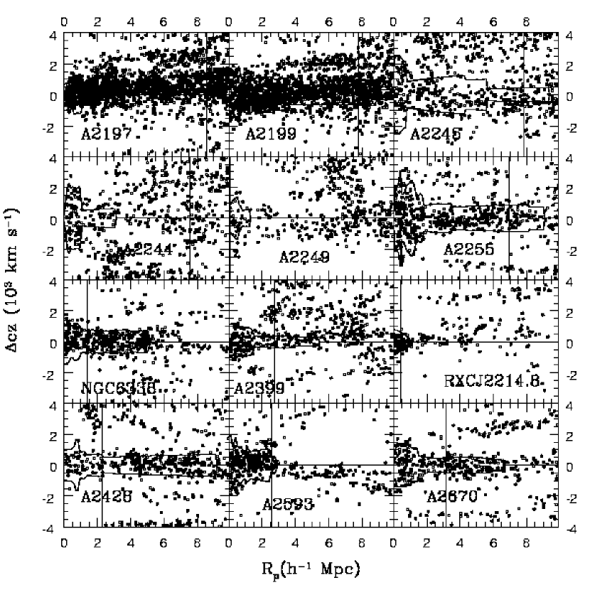
Figure 7: See Figure 2.

The spectroscopic limit of the main galaxy sample of SDSS is $r$=17.77 after correcting for Galactic extinction (Strauss et al., 2002). CAIRNS sampled all galaxies brighter than about $M^{*}+1$ and often fainter. Figure 7 of Rines et al. (2005) shows the infall patterns for galaxies brighter than $M_{K_{s}}^{*}+1$. These patterns are readily apparent, but less well-defined than the full CAIRNS samples (Rines et al., 2003). Assuming the luminosity function of Blanton et al. (2003), the spectroscopic limit of SDSS corresponds to $M_{{}^{0.1}r}^{*}+1$ at $z=0.092$. Thus, we expect that infall patterns of clusters with masses similar to CAIRNS clusters should be apparent to $z\lesssim$0.1, though not much further.

Note that the SDSS Main Galaxy Survey is $\sim$85-90% complete to the spectroscopic limit. The survey has $\approx$7% incompleteness due to fiber collisions (Strauss et al., 2002), which are likely more common in dense cluster fields. Because the target selected in a fiber collision is determined randomly, this incompleteness can theoretically be corrected for in later analysis. From a comparison of SDSS with the Millennium Galaxy Catalogue, Cross et al. (2004) conclude that there is an additional incompleteness of $\sim$7% due to galaxies misclassified as stars or otherwise missed by the SDSS photometric pipeline. For our purposes, the incompleteness is not important provided sufficient numbers of cluster galaxies do have spectra.

2.2 X-ray Cluster Surveys

Because SDSS surveys primarily low-redshift galaxies, the best sampled clusters are both nearby and massive. We therefore search X-ray cluster catalogs derived from the ROSAT All-Sky Survey for clusters in DR4. RASS (Voges et al., 1999) is a shallow survey but it is sufficiently deep to include nearby, massive clusters. RASS covers virtually the entire sky and is thus the most complete X-ray cluster survey for nearby clusters. RASS was conducted with the PSPC (Position Sensitive Proportional Counter) instrument.

Published cluster catalogs derived from the RASS include the X-ray Brightest Abell Cluster Survey (XBACS), the Bright Cluster Survey (BCS), the NOrthern ROSAT All-Sky galaxy cluster survey (NORAS), and the ROSAT-ESO flux limited X-ray galaxy cluster survey (REFLEX). XBACS is “an essentially complete, all-sky, X-ray flux-limited sample of 242 Abell clusters” from RASS I (Ebeling et al., 1996), the first processing of the RASS. BCS is the Bright Cluster Survey (Ebeling et al., 2000b) and eBCS is an extension of this survey to a smaller limiting flux (Ebeling et al., 2000a). XBACs and BCS/eBCS were constructed first by searching for X-ray sources around known optical clusters from the Abell and Zwicky catalogs; they then use a Voronoi Tesselation and Percolation (VTP) algorithm to identify extended X-ray sources (from a master catalog of X-ray point sources) not associated with optical clusters. PSPC count rates are converted to total fluxes (in the 0.1-2.4 keV energy band) using King models to account for missing flux at large radii and corrected for Galactic absorption and $K$ corrected using either temperatures from David et al. (1993) or a correction from the $L_{X}-T$ relation from an iterative process. BCS/eBCS covers the northern hemisphere at high Galactic latitudes ($\delta\geq$0^∘ and $|b|>$20^∘). The flux limits of BCS and eBCS are 4.4 and 2.8$\times 10^{-12}$erg s^-1 cm^-2 respectively. Ebeling et al. (2000b) estimate the completeness to these limits is approximately 90% and 80%, where the missing clusters are extended sources not included in the master catalog of X-ray point sources.

NORAS (Böhringer et al., 2000a) also covers the northern hemisphere at high Galactic latitudes ($\delta\geq$0^∘ and $|b|>$20^∘). The initial source catalog consists of extended objects detected in RASS I with their properties determined from RASS II (the second processing of RASS, Voges et al., 1999) data. The fluxes are computed using a method called growth curve analysis and are corrected for missing flux by fitting the emission profile to a $\beta$ model (Cavaliere & Fusco-Femiano, 1976) and extrapolating to 12 core radii. The NORAS fluxes agree well with BCS/eBCS fluxes for clusters in common. Both surveys are expected to be incomplete. Comparing NORAS and REFLEX, Böhringer et al. (2000b) estimate that the completeness of NORAS is about 50%. In a subset of NORAS (an area of sky between right ascensions 9^h and 14^h and declinations $\delta$$>$0), the completeness increases to 82% with the addition of several additional clusters found in a thorough search of Abell cluster positions and extended sources in the RASS II catalog Böhringer et al. (2000b). We include these clusters in our sample.

REFLEX (Böhringer et al., 2001, 2004) is analogous to NORAS but for the southern hemisphere. Both NORAS and REFLEX extend to smaller X-ray fluxes than XBACS. The catalog construction is different for each survey: XBACs and BCS/eBCS initially search for extended X-ray sources around known optical clusters; BCS/eBCS includes additional X-ray selected clusters selected from a master catalog of point sources. NORAS is selected from extended X-ray sources with no explicit optical selection. Finally, REFLEX matches X-ray flux overdensities with galaxy overdensities and is therefore selected jointly in X-ray and optical wavelengths. The REFLEX fluxes are calculated in the same manner as NORAS.

When multiple X-ray fluxes are available for a cluster, we use the most recently published value. The order of preferences is therefore: REFLEX, NORAS, BCS/eBCS, XBACs. We define a flux-limited and redshift-limited sample of clusters with the criteria $f_{X}\geq 3\times 10^{-12}$erg s^-1cm^-2 (0.1-2.4 keV) and $z\leq$0.10. Note that variations in the method of determining flux in different catalogs may affect the precise flux limit. The only cluster with an XBACs flux is A1750b, the southern component of A1750. We follow Böhringer et al. (2004) and treat A1750 as a single source rather than two separate sources as in XBACs. Similarly, the galaxy NGC5813 is bound to the NGC5846 group (Mahdavi et al., 2005). Because the dynamics of NGC5813 are dominated by the NGC5846 system, we eliminate NGC5813 from the sample. We inspect the redshift data around each cluster to confirm the cluster redshift and find that A2064 has an incorrect redshift (and X-ray luminosity) listed in NORAS. The correct redshift is 0.0738 instead of 0.1076. We correct the X-ray luminosity accordingly. The redshift of A2149 is listed as $z$=0.1068 in NORAS and $z$=0.0675 in eBCS. Because the X-ray peak of the RASS image lies near an apparent BCG at the latter redshift (see $\S$4), we adopt the eBCS value and adjust the X-ray luminosity accordingly. Our final flux and redshift limited sample contains 72  clusters within the SDSS DR4 spectroscopic footprint. We will refer to this sample as the CIRS (Cluster Infall Regions in SDSS) clusters hereafter. The completeness of the CIRS sample is limited by the completeness of the underlying cluster catalogs. However, by combining clusters from the various catalogs we should be more complete than any individual catalog. For our purposes, this modest potential incompleteness is not important. The clusters are an unbiased sample: the selection of the CIRS sample is based purely on X-ray flux and the footprint of the SDSS DR4 spectroscopic survey.

3 Results

3.1 Ubiquity of Infall Patterns around Clusters

We first test for the ubiquity of caustic or infall patterns around X-ray clusters. Analogous to CAIRNS, we plotted radius-redshift diagrams for all clusters in the X-ray cluster catalogs covered by DR4 with $z<$0.20. Clusters with $z>$0.10 have few spectroscopically confirmed members in DR4 (see $\S$2.1). The caustic pattern is a superposition of the “finger-of-God” elongation in redshift space of the virialized galaxies in the cluster center and the flattening due to infall at large radii. The resulting infall pattern is a characteristic trumpet shape in phase space (Kaiser, 1987, D99). Substructure in the infall region smears out the sharp enhancements in phase space predicted by simple spherical infall, so the infall pattern should be apparent as a dense envelope of galaxies in phase space with well-defined edges (D99). The detailed appearance of the redshift-radius diagrams depends on the line-of-sight of the observer, so the contrast between the dense infall envelope and foreground and background galaxies is subject to projection effects (D99). We assign a “by-eye” classification of each cluster’s infall pattern: “clean” for clusters with few background and foreground galaxies, “intermediate” for clusters with apparent infall patterns but significant contamination from either related large-scale structure or foreground and background objects, and “none” for clusters with no apparent infall pattern. Below, we demonstrate that the caustic technique can be applied successfully to clusters classified here as “intermediate” or “none”; our classification scheme is thus fairly conservative. We use this classification scheme only to show the dependence of the infall pattern appearance on cluster mass and the sampling depth.

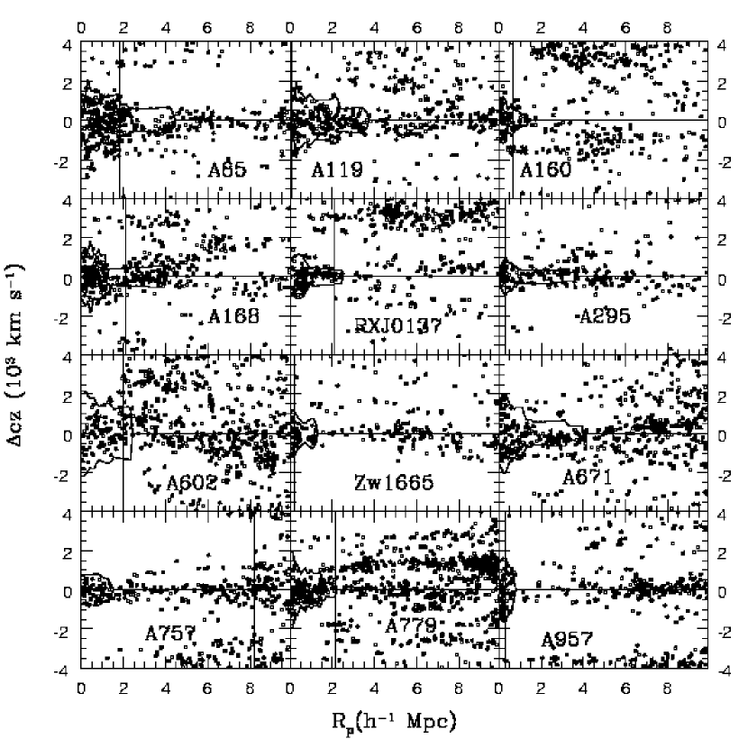
Figure 2: Redshift versus radius for SDSS galaxies around the first twelve X-ray clusters in the CIRS sample. The caustic pattern is evident as the trumpet-shaped regions with high density. The solid lines indicate our estimate of the location of the caustics in each cluster. Vertical lines in each panel indicate the radius where the spatial coverage of the SDSS DR4 spectroscopic survey is no longer complete. Figures 3-7 show similar plots for the rest of the sample.

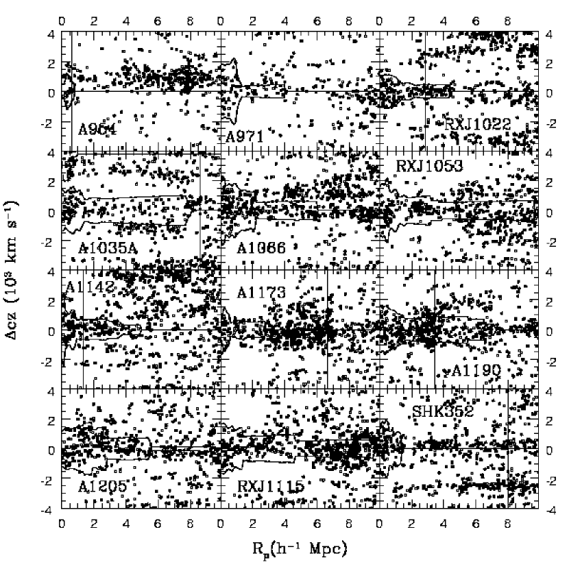
Figure 3: See Figure 2. The dashed lines in the diagram for A1035A indicate the infall pattern of a higher-redshift component.

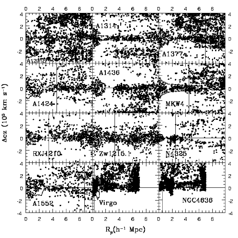
Figure 4: See Figure 2. The dashed lines in the diagram for A1291B indicate the infall pattern of a lower-redshift component.

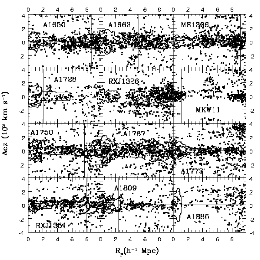
Figure 5: See Figure 2.

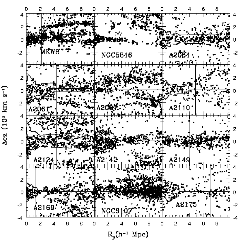
Figure 6: See Figure 2.

Figure 1 shows the dependence of this subjective classification on X-ray luminosity and redshift. As expected from the depth of SDSS ($\S\ref{sdssdesc}$), there are few “clean” infall patterns where SDSS samples shallower than $M_{*}+1$. We therefore define a “complete” sample selected by X-ray flux $f_{X}\geq 3\times 10^{-12}$erg s^-1cm^-2 (0.1-2.4 keV) and redshift ($z\leq$0.10). The CIRS sample contains 72  clusters; the vast majority of this sample (56/72  or 78%) contain “clean” infall patterns and only three (4%) show no obvious infall pattern. Of the three clusters in the latter category, two are embedded in larger structures (NGC4636 in the outskirts of the Virgo cluster and A2067 in the outskirts of A2061, part of the CorBor supercluster) and one (A1291) is a possible merging cluster with two nearly concentric components separated by $\sim$2000 ${\rm km~{}s}^{-1}$ (see $\S$4 for details). In $\S$3.2 we are able to identify caustics in 100% of the CIRS clusters. Figure 1 also shows the CAIRNS X-ray luminosity and redshift limits. The three CIRS clusters meeting this criteria were studied by CAIRNS (A119, A168, and A2199). Figure 1 demonstrates the expanded parameter space covered by the CIRS sample. Table 1 lists the clusters in the CIRS sample, their X-ray positions, luminosities, and temperatures (when available), their central redshifts and velocity dispersions (see below), and the projected radius $R_{comp}$ within which the SDSS DR4 spectroscopic survey provides complete spatial coverage. For several clusters, the caustic pattern disappears beyond $R_{comp}$ because of this edge effect. Figures 2-7 show the radius-redshift diagrams for the CIRS sample. Vertical lines in some panels indicate the radius within which the DR4 spectroscopic footprint provides complete coverage of the infall region; the absence of a caustic pattern in some clusters beyond this limit is due to incomplete spatial coverage.

Another factor which determines the presence or absence of a “clean” infall pattern is the surrounding large-scale structure. For example, the redshift-radius diagrams of groups within the infall regions of more massive clusters reflect the kinematics of the cluster’s infall region (e.g., A2199, see Rines et al., 2002). The CIRS sample contains several of these systems: NGC6107 and A2197 in the infall region of A2199, NGC4636 in the infall region of Virgo, NGC5813 in the infall region of NGC5846, and A2067 in the infall region of A2061. A1173 and A1190 are close and likely bound. Two clusters, A1035 and A1291, show evidence of two infall patterns in the projected radius-redshift diagrams. We label the two components A and B with A indicating the lower redshift component. The caustic algorithm finds A1035B and A1291A to be the larger components; we use these components when compiling results for the CIRS sample. We discuss these systems in more detail in $\S\ref{individual}$.

3.2 Caustics and Mass Profiles

Similar to CAIRNS, the CIRS clusters show infall patterns much more well defined than those of the simulations of D99. Because infall patterns are better defined in a low-density universe (D99), a possible explanation for this discrepancy is that the real universe has a smaller matter density than the simulations. Another possibility is that the semi-analytic galaxy formation recipes used in D99 are inaccurate around massive clusters.

We briefly review the method DG and D99 developed to estimate the mass profile of a galaxy cluster by identifying caustics in redshift space. The method assumes that clusters form in a hierarchical process. Application of the method requires only galaxy redshifts and sky coordinates. Toy models of simple spherical infall onto clusters produce sharp enhancements in the phase space density around the system. These enhancements, known as caustics, appear as a trumpet shape in scatter plots of redshift versus projected clustercentric radius (Kaiser, 1987; Regös & Geller, 1989). DG and D99 show that random motions smooth out the sharp pattern expected from simple spherical infall into a dense envelope in the redshift-radius diagram (see also Vedel & Hartwick, 1998). The edges of this envelope can be interpreted as the escape velocity as a function of radius. Galaxies outside the caustics are also outside the turnaround radius. The caustic technique provides a well-defined boundary between the infall region and interlopers; one may think of the technique as a method for defining membership that gives the cluster mass profile as a byproduct.

The amplitude $\mathcal{A}\mathnormal{(r)}$ of the caustics is half of the distance between the upper and lower caustics in redshift space. Assuming spherical symmetry, $\mathcal{A}\mathnormal{(}r)$ is related to the cluster gravitational potential $\phi(r)$ by

$$\mathcal{A}\mathnormal{{}^{2}(r)=-2\phi(r)\frac{1-\beta(r)}{3-2\beta(r)}}$$ (1)

where $\beta(r)=1-[\sigma_{\theta}^{2}(r)/\sigma_{r}^{2}(r)]$ is the velocity anisotropy parameter and $\sigma_{\theta}$ and $\sigma_{r}$ are the tangential and radial velocity dispersions respectively. DG show that the mass of a spherical shell of radii [$r_{0},r$] within the infall region is the integral of the square of the amplitude $\mathcal{A}\mathnormal{(r)}$

$$GM(<r)-GM(<r_{0})=F_{\beta}\int_{r_{0}}^{r}\mathcal{A}\mathnormal{{}^{2}(x)dx}$$ (2)

where $F_{\beta}\approx 0.5$ is a filling factor with a numerical value estimated from simulations. Variations in $F_{\beta}$ lead to some systematic uncertainty in the derived mass profile (see D99 for a more detailed discussion). Note that the variations in $F_{\beta}$ are included in the estimates of the systematic uncertainties in the caustic technique.

Operationally, we identify the caustics as curves which delineate a significant decrease in the phase space density of galaxies in the projected radius-redshift diagram. For a spherically symmetric system, taking an azimuthal average amplifies the signal of the caustics in redshift space and smooths over small-scale substructures. We isolate the clusters initially by studying only galaxies within $R_{p}\leq$10$h^{-1}{\rm Mpc}$ and $\pm$5000${\rm km~{}s}^{-1}$ of the nominal cluster centers from the X-ray catalogs. We perform a hierarchical structure analysis to locate the centroid of the largest system in each volume (see Appendix A of D99). This analysis consists of creating a binary tree based on estimated binding energies, identifying the largest cluster in the field, and determining its center from the two-dimensional distribution of celestial coordinates determined with adaptive kernel smoothing. This analysis sometimes finds the center of another system in the field. In these cases, limiting the galaxies to a smaller radial and/or redshift range enables the algorithm to center on the desired cluster. Table 4 lists these restrictions.

We adaptively smooth the azimuthally averaged phase space diagram (the ensemble of redshift, radius data points) and the algorithm chooses a threshold in phase space density as the edge of the caustic envelope. The upper and lower caustics at a given radius are the redshifts at which this threshold density is exceeded when approaching the central redshift from the “top” and “bottom” respectively of the redshift-radius diagram. Because the caustics of a spherical system are symmetric, we adopt the smaller of the upper and lower caustics as the caustic amplitude $\mathcal{A}\mathnormal{(r)}$ at that radius. This procedure reduces the systematic uncertainties introduced by interlopers, which generally lead to an overestimate of the caustic amplitude. The threshold is defined by the algorithm to minimize the quantity $|<$$v_{esc}^{2}$$>_{R}-4<$$v^{2}$$>_{R}|$, where R is a virial-like radius (see D99 for details). Rines et al. (2002) explore the effects of altering some of these assumptions and find that the differences are generally smaller than the estimated uncertainties.

D99 described this method in detail and showed that, when applied to simulated clusters containing galaxies modelled with semi-analytic techniques, it recovers the actual mass profiles to radii of 5-10$~{}h^{-1}{\rm Mpc}$ from the cluster centers. D99 gives a prescription for estimating the uncertainties in the caustic mass profiles. The uncertainties estimated using this prescription reproduce the actual differences between the caustic mass profiles and the true mass profiles of the simulated clusters including systematic effects such as departures from spherical symmetry. The uncertainties in the caustic mass profiles of observed clusters may be smaller than the 50% uncertainties in the simulations (Rines et al., 2003). This difference is due in part to the large number of redshifts in the CIRS redshift catalogs relative to the simulated catalogs. Furthermore, the caustics are generally more cleanly defined in the data than in the simulations. Clearly, more simulations which better reproduce the appearance of observed caustics and/or include fainter galaxies would be useful in determining the limits of the systematic uncertainties in the caustic technique. We are currently conducting an analysis for the hydrodynamical simulations of Borgani et al. (2004) with these goals (A. Diaferio et al. 2006, in preparation).

We calculate the shapes of the caustics with the technique described in D99 using a smoothing parameter of $q$=25. The smoothing parameter $q$ is the scaling between the velocity smoothing and the radial smoothing in the adaptive kernel estimate of the underlying phase space distribution (e.g., a particle which has a smoothing window in the radial direction of 0.04$h^{-1}$Mpc will have a smoothing window in the velocity direction of 100 ${\rm km~{}s}^{-1}$ for $q$=25 and 40 ${\rm km~{}s}^{-1}$ for $q$=10). Previous investigations show that the mass profiles are insensitive to changes of a factor of 2 in the smoothing parameter (Geller et al., 1999; Rines et al., 2000, 2002).

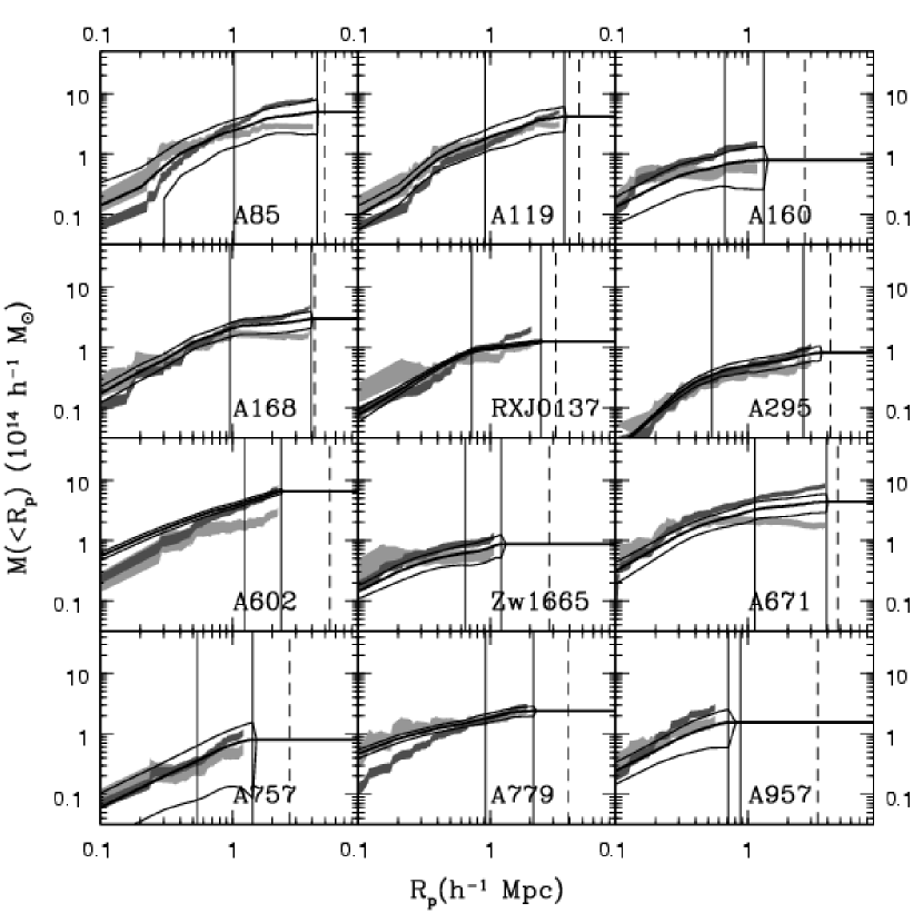
Figure 18: Comparison of caustic mass profiles to those estimates from the virial theorem and the projected mass estimator. The thick solid lines show the caustic mass profiles and the thin lines show the 1$\sigma$ uncertainties in the mass profiles. The axes are identical in all panels. The vertical bars indicate $r_{200}$ and the maximum radius of the caustic mass profile (the smaller of $r_{max}$, the extent of the infall pattern, and $r_{t}$, the turnaround radius). Vertical dashed lines indicate $r_{t}$ for clusters where the infall pattern truncates before $r_{t}$. Red and green shaded regions show the formal 1$\sigma$ uncertainties in the virial and projected mass profiles. Figures 19-23 show similar plots for the rest of the sample.

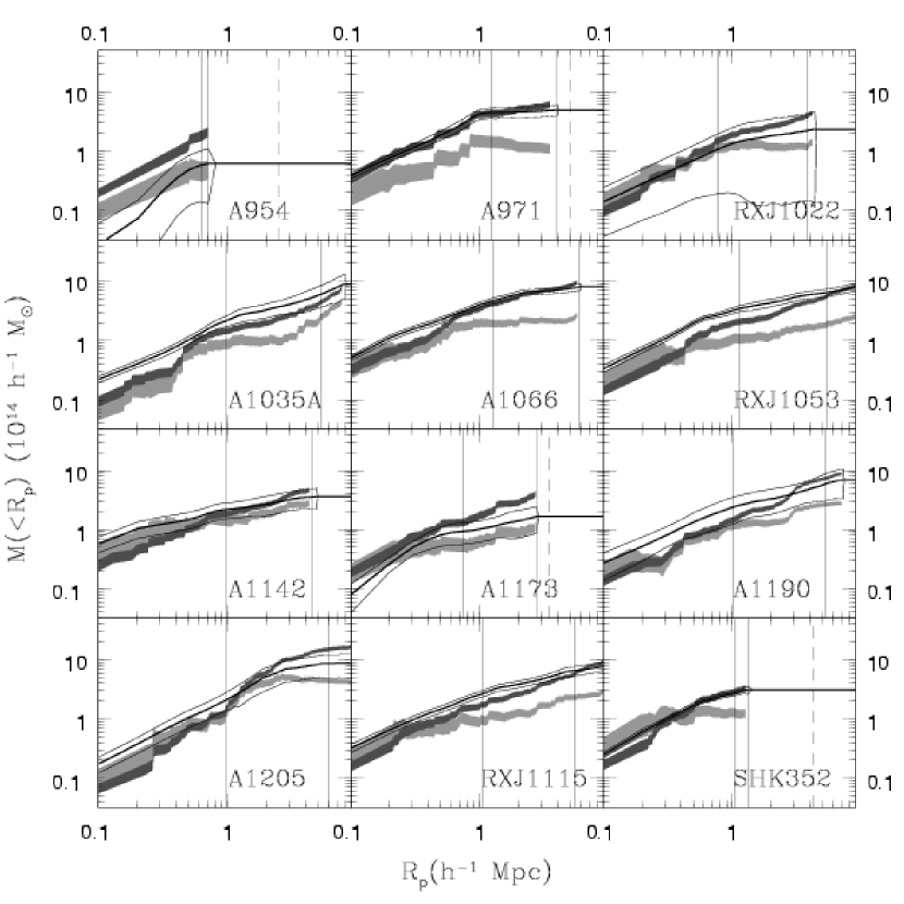
Figure 19: See Figure 18.

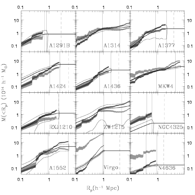
Figure 20: See Figure 18.

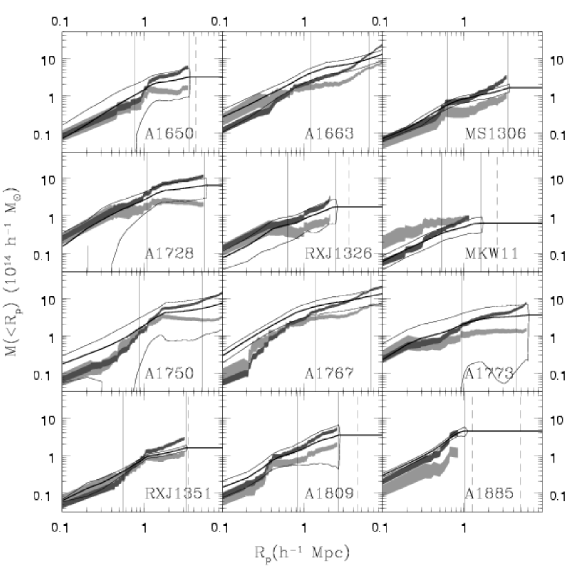
Figure 21: See Figure 18.

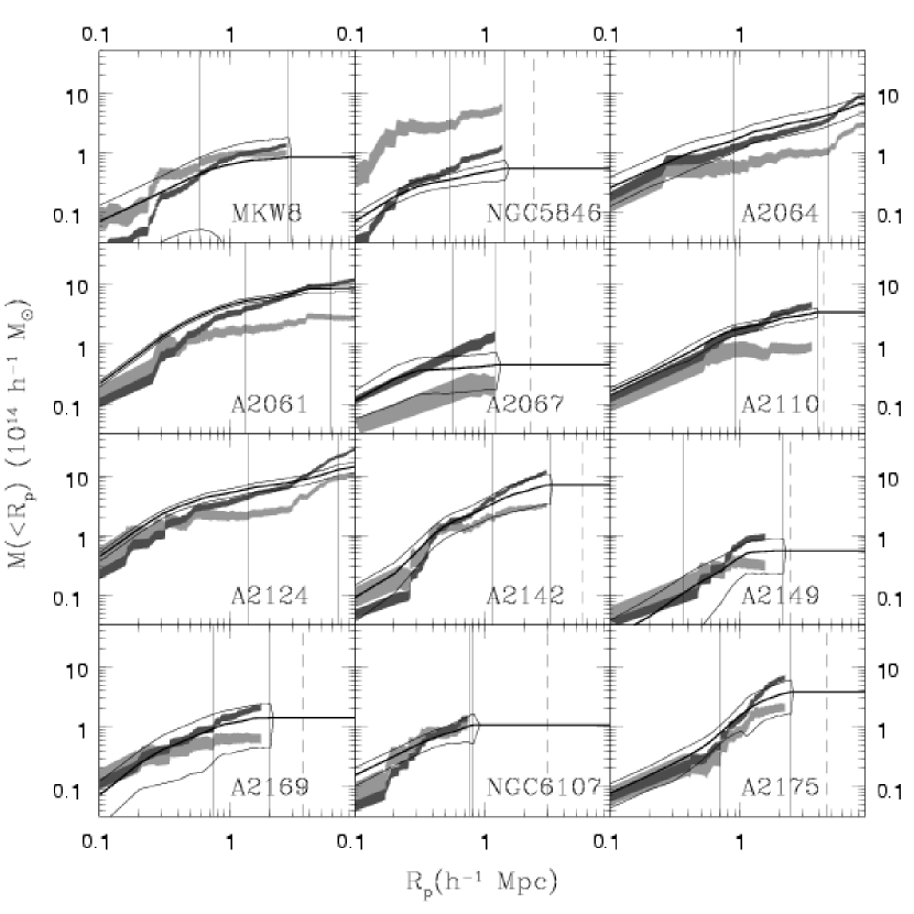
Figure 22: See Figure 18.

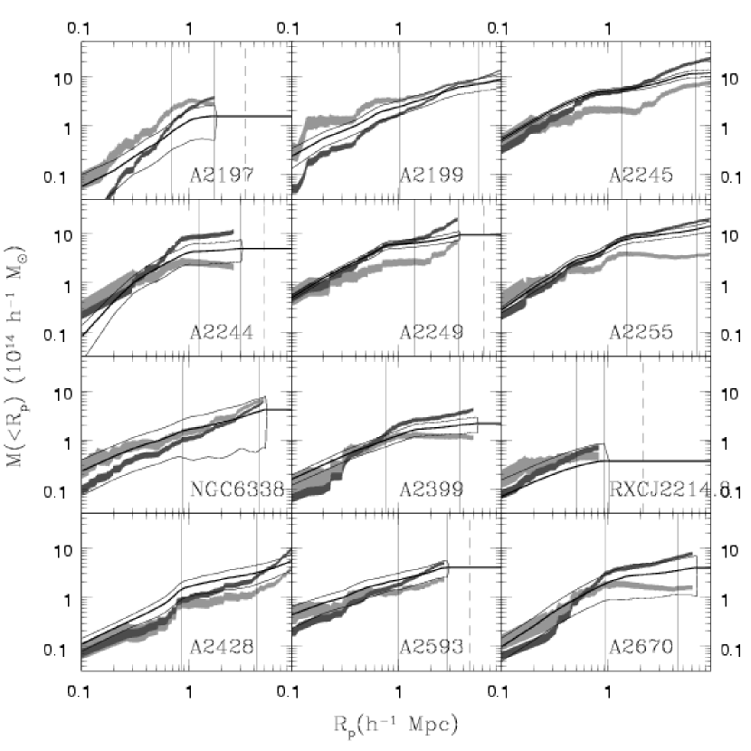
Figure 23: See Figure 18.

Table 2 lists the hierarchical centers. These centers generally agree with the X-ray positions (Table 2) with a median difference of 109$~{}h^{-1}{\rm kpc}$ and with the redshift centers from the X-ray catalogs with a median difference of -17 ${\rm km~{}s}^{-1}$. The hierarchical centers disagree by more than 500$h^{-1}{\rm kpc}$ in four clusters and by more than 1000 ${\rm km~{}s}^{-1}$ for seven clusters. The hierarchical redshift centers are more reliable than those in the X-ray cluster catalogs because the former are based on much larger redshift samples. We discuss some of the individual cases in $\S$4. Figures 2-7 show the caustics and Figures 18-23 show the associated mass profiles. Note that the caustics extend to different radii for different clusters. D99 show that the appearance of the caustics depends strongly on the line of sight; projection effects can therefore account for most of the differences in profile shape in Figures 2-7 without invoking non-homology among clusters. The uncertainties in the caustic mass profiles are estimated with the prescription of D99 for Coma-size clusters. Under this prescription, more densely sampled clusters and those with higher contrast between the caustics and the background have smaller uncertainties than sparsely sampled clusters or those with poorer contrast. Thus, the uncertainties in the caustic mass profiles for some CIRS clusters (those with smaller masses or unusually empty backgrounds) computed with this prescription may underestimate the total systematic uncertainties.

We use the caustics to determine cluster membership. Here, the term “cluster member” refers to galaxies both in the virial region and in the infall region. Figures 2-7 show that the caustics effectively separate cluster members from background and foreground galaxies, although some interlopers may lie within the caustics. This clean separation affirms our adoption of velocity dispersions calculated from cluster members as defined by the caustics ($\S$3.2).

We find a measureable signal for the caustic profile for all 72 X-ray clusters in the CIRS sample (that is, all show an identifiable cluster of galaxies with a surrounding infall pattern). This amazing success rate demonstrates the power and ubiquity of the caustic technique in identifying the galaxies associated with clusters and their infall regions.

In the simulations of D99, the degree of definition of the caustics depends on the underlying cosmology; caustics are better defined in a low-density universe than a flat, matter-dominated universe. Surprisingly, the contrast of the phase space density between regions inside and outside the caustics is much stronger in the data than in both the $\tau$CDM and $\Lambda$CDM simulated clusters in D99. The difference may arise from the cosmological model used or the semi-analytic techniques for defining galaxy formation and evolution in the simulations. The difference may be accentuated by the large numbers of redshifts in the CIRS catalogs which extend (non-uniformly) to fainter magnitudes than the simulated catalogs displayed in D99. The contrast of the caustics with the background is unlikely to be a precise cosmological indicator, but it is suggestive that real clusters more closely resemble the $\Lambda$CDM than the $\tau$CDM simulated cluster.

The caustic patterns in the CAIRNS clusters are robust to the addition of fainter galaxies to the radius-redshift diagrams (Geller et al., 1999; Rines et al., 2003). This result suggests that dwarf galaxies trace the same caustic pattern as giant galaxies. This result holds for the CIRS clusters; in particular, A2199, a CAIRNS cluster, has much deeper sampling in CIRS (double the redshifts in CAIRNS), yet the mass profiles agree quite well. These results imply that any velocity bias on the scale of infall regions does not depend strongly on galaxy luminosity.

We discuss some individual clusters in more detail in $\S\ref{individual}$.

3.3 Virial and Turnaround Masses and Radii

The caustic mass profiles allow direct estimates of the virial and turnaround radius in each cluster. For the virial radius, we estimate $r_{200}$ ($r_{\Delta}$ is the radius within which the enclosed average mass density is $\Delta\rho_{c}$, where $\rho_{c}$ is the critical density) by computing the enclosed density profile [$\rho(<r)=3M(<r)/4\pi r^{3}$]; $r_{200}$ is the radius which satisfies $\rho(<r_{200})=200\rho_{c}$. In our adopted cosmology, a system should be virialized inside the slightly larger radius $\sim$$r_{100}\approx 1.3r_{200}$ (Eke et al., 1996). We use $r_{200}$ because it is more commonly used in the literature and thus allows easier comparison of results. For the turnaround radius $r_{t}$, we use equation (8) of Regös & Geller (1989) assuming $\Omega_{m}=0.3$. For this value of $\Omega_{m}$, the enclosed density is 3.5$\rho_{c}$ at the turnaround radius. If the $w$ parameter in the equation of state of the dark energy ($P_{\Lambda}=w\rho_{\Lambda}$) satisfies $w\geq-1$, the dark energy has little effect on the turnaround overdensity (Gramann & Suhhonenko, 2002). Varying $\Omega_{m}$ in the range 0.02–1 only changes the inferred value of $r_{t}$ by $\pm$10%; the uncertainties in $r_{t}$ from the uncertainties in the mass profile are comparable or larger (Rines et al., 2002).

Table 3 lists $r_{200}$, $r_{t}$, and the masses $M_{200}$ and $M_{t}$ enclosed within these radii. For some clusters, the maximum extent of the caustics $r_{max}$ is smaller than $r_{t}$. For these clusters, $r_{t}$ is a lower bound calculated assuming that there is no additional mass outside $r_{max}$. The best estimate of the mass contained in infall regions clearly comes from those clusters for which $r_{max}\geq r_{t}$. The average mass within the turnaround radius for these clusters is 2.19$\pm$0.18 times the virial mass $M_{200}$ (the average ratio for all clusters is 1.97$\pm$0.10). The average turnaround radius is (4.96$\pm$0.08)$r_{200}$ for clusters with $r_{max}\geq r_{t}$, and (4.75$\pm$0.07)$r_{200}$ averaged over all clusters. Simulations of the future growth of large-scale structure (Lahav et al., 1991; Gramann & Suhhonenko, 2002; Nagamine & Loeb, 2003; Busha et al., 2003) for our assumed cosmology ($\Omega_{m}=0.3,\Omega_{\Lambda}=0.7$) suggest that galaxies currently inside the turnaround radius of a system will continue to be bound to that system. In open cosmologies with $\Omega_{\Lambda}=0$, objects in regions where the enclosed density exceeds the critical density are bound, whereas in closed cosmologies, all objects are bound to all other objects. Busha et al. (2005) find that the ultimate mass of dark matter haloes in $\Lambda$CDM simulations is, on average, 1.9 times their masses $M_{200}$ measured at $z$=0. Our measure of $M_{t}/M_{200}$=2.19$\pm$0.18 confirms their numerical prediction, if we expect that all the mass within $r_{t}$ will eventually fall onto the cluster. We compare the virial masses $M_{200}$ from the caustics with masses calculated using the virial theorem in $\S 7$.

One striking result of this analysis is that the caustic pattern is often visible beyond the turnaround radius of a cluster. This result suggests that clusters may have strong dynamic effects on surrounding large-scale structure beyond the turnaround radius. For our assumed cosmology, this large-scale structure is probably not bound to the cluster. See Plaga (2005) for an alternative explanation of this observed structure.

3.4 Cluster Scaling Relations

Scaling relations between simple cluster observables and masses provide insight into the nature of cluster assembly and the properties of various cluster components. Establishing these relations for local clusters is critical for future studies of clusters in the distant universe with the goal of constraining dark energy (Majumdar & Mohr, 2004; Lin et al., 2004).

We apply the prescription of Danese et al. (1980) to determine the mean redshift $cz$ and projected velocity dispersion $\sigma_{p}$ of each cluster from all galaxies within the caustics. We calculate $\sigma_{p}$ using only the cluster members projected within $r_{200}$ estimated from the caustic mass profile. Note that our estimates of $r_{200}$ do not depend on $\sigma_{p}$.

One of the simplest observables of clusters is X-ray luminosity. The X-ray luminosities are in the ROSAT band (0.1-2.4 keV) and corrected for Galactic absorption (taken from REFLEX, NORAS, and BCS/eBCS). Figure 8 shows the $L_{X}-\sigma_{p}$ relation for the CIRS clusters along with the best-fit $L_{X}-\sigma_{p}$ relation of the RASS-SDSS (Popesso et al., 2005). Although the scatter is large, the CIRS clusters follow the same relation as the RASS-SDSS sample.

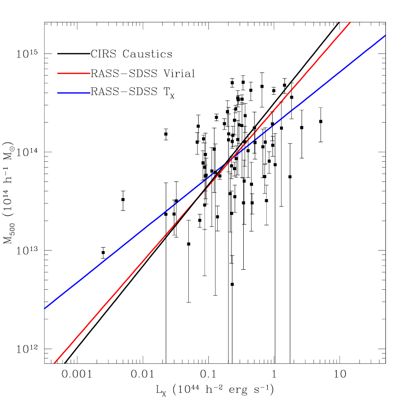
Figure 9: Caustic masses at $r_{500}$ compared to X-ray luminosities. The solid line is the bisector of the ordinary least squares fits. The red and blue lines show the $M_{500}-L_{X}$ relations for RASS-SDSS (Popesso et al., 2005) for optical and X-ray masses respectively.

Figure 9 shows $L_{X}$ versus $M_{500}$ as estimated from the caustics. The bisector of the least-squares fits to the CIRS sample agrees very well with the RASS-SDSS $M_{500}-L_{X}$ relation for masses estimated with the virial theorem (Popesso et al., 2005), but both relations are offset from the $M_{500}-L_{X}$ relation with masses estimated from $T_{X}$. The significance and origin of this offset merit a more detailed analysis than possible here.

The mass-temperature relation (Evrard et al., 1996; Horner et al., 1999; Nevalainen et al., 2000; Finoguenov et al., 2001) gives a straightforward estimate of the mass of a cluster from its X-ray temperature. We use the mass-temperature relation rather than, e.g., a $\beta$ model to estimate the mass both for simplicity and to ensure uniformity (X-ray observations allowing more detailed mass estimates are only available for a small fraction of the CIRS clusters). Numerical simulations (Evrard et al., 1996) suggest that estimating cluster masses based solely on emission-weighted cluster temperatures yields similar accuracy and less scatter than estimates which incorporate density information from the surface brightness profile.

Figure 10 shows the X-ray temperature versus $M_{500}$ as estimates from the caustics for a subset of 28 clusters with X-ray temperatures listed in Jones & Forman (1999) or Horner (2001). The solid line is the bisector of the least-squares fits; the other lines show the best-fit relations of Finoguenov et al. (2001) and RASS-SDSS (Popesso et al., 2005). We again find excellent agreement with previously determined scaling relations.

Figure 11 shows the $M_{200}-\sigma_{p}$ relation. The tight relation indicates that the caustic masses are well correlated with velocity dispersion estimates. The good correlation is perhaps not surprising because both parameters depend on the galaxy velocity distribution. The best-fit slope is $M_{200}\propto\sigma_{p}^{3.18\pm 0.19}$ with the uncertainty estimated from jackknife resampling. We compare the caustic masses to virial mass estimates in $\S$6.

The excellent agreement between the caustic masses and the X-ray masses from previously determined scaling relation between mass and X-ray temperatures confirms the prediction of D99 that the caustic mass estimate is unbiased. CAIRNS found similar agreement between caustic masses and X-ray and virial mass estimates (Rines et al., 2003); Diaferio et al. (2005) show good agreement between masses estimated from the caustics and weak lensing.

3.5 The Shapes of Cluster Mass Profiles

We fit the mass profiles of the CAIRNS clusters to three simple analytic models. The simplest model of a self-gravitating system is a singular isothermal sphere (SIS). The mass of the SIS increases linearly with radius. Navarro et al. (1997) and Hernquist (1990) propose two-parameter models based on CDM simulations of haloes. We note that the caustic mass profiles mostly sample large radii and are therefore not very sensitive to the inner slope of the mass profile. Thus, we do not consider alternative models which differ only in the inner slope of the density profile (e.g., Moore et al., 1999). At large radii, the best constraints on cluster mass profiles come from galaxy dynamics and weak lensing. The caustic mass profiles of Coma (Geller et al., 1999), A576 (Rines et al., 2000), A2199 (Rines et al., 2002) and the rest of the CAIRNS clusters (Rines et al., 2003) provided strong evidence against a singular isothermal sphere (SIS) profile and in favor of steeper mass density profiles predicted by Navarro et al. (1997) (NFW) and Hernquist (1990). Only recently have weak lensing mass estimates been able to distinguish between SIS and NFW density profiles at large radii (Clowe & Schneider, 2001; Kneib et al., 2003).

At large radii, the NFW mass profile increases as ln$(r)$ and the mass of the Hernquist model converges. The NFW mass profile is

$$M(<r)=\frac{M(a)}{\mbox{ln}(2)-\frac{1}{2}}[\mbox{ln}(1+\frac{r}{a})-\frac{r}{a+r}]$$ (3)

where $a$ is the scale radius and $M(a)$ is the mass within $a$. We fit the parameter $M(a)$ rather than the characteristic density $\delta_{c}$ (${M(a)=4\pi\delta_{c}\rho_{c}a^{3}[\mbox{ln}(2)-\frac{1}{2}]}$ where $\rho_{c}$ is the critical density) because $M(a)$ and $a$ are much less correlated than $\delta_{c}$ and $a$ (Mahdavi et al., 1999). The Hernquist mass profile is

$$M(<r)=M\frac{r^{2}}{(r+a_{H})^{2}}$$ (4)

where $a_{H}$ is the scale radius and $M$ is the total mass. Note that $M(a_{H})=M/4$. The SIS mass profile is $M(<r)\propto r$. We minimize $\chi^{2}$ and list the best-fit parameters $a$, $r_{200}$, the concentration $c_{NFW}$=$r_{200}/a$, and $M_{200}$ for the best-fit NFW model and indicate the best-fit profile type in Table 5. We also list the parameter $c_{101}$=$r_{101}/a$; some authors prefer to use $r_{101}$ as the virial radius. We perform the fits on all data points within the maximum radial extent of the caustics $r_{max}$ listed in Table 3 and with caustic amplitude $\mathcal{A}\mathnormal{(r)}>100~{}{\rm km~{}s}^{-1}$.

Because the individual points in the mass profile are not independent, the absolute values of $\chi^{2}$ are indicative only, but it is clear that the NFW and Hernquist profiles provide acceptable fits to the caustic mass profiles; the SIS is excluded for nearly all clusters. The NFW profile provides a better fit to the data than the Hernquist profile for 36 of the 72 CIRS clusters; 35 are better fit by a Hernquist profile and one is best fit by SIS. A non-singular isothermal sphere mass profile yields results similar to the SIS; thus, we report only our results for the SIS.

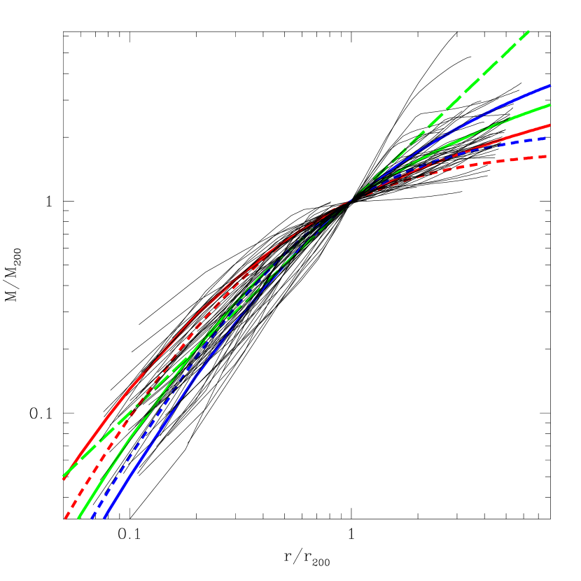
Figure 12: Scaled caustic mass profiles for the CIRS clusters compared to simple models. The thin solid lines show the caustic mass profiles normalized by $r_{200}$ and $M_{200}$. The long-dashed line shows a singular isothermal sphere, the colored solid lines show NFW profiles (with concentrations $c$=3,5,10 from top to bottom at large radii). The short-dashed lines are Hernquist profiles with scale radii different by a factor of two.

Figure 12 shows the shapes of the caustic mass profiles scaled by $r_{200}$ and $M_{200}$ along with SIS, NFW, and Hernquist model profiles. The colored lines show different model mass profiles. The straight dashed line is the SIS, the solid lines are NFW profiles with $c$=3,5, and 10, and the curved dashed lines are Hernquist profiles with two different scale radii. The best-fit average profile is an NFW profile with $c_{200}$=7.2 (this lowers to $c_{200}$=5.2 when the fits are restricted to $r$$\leq$$r_{200}$), consistent with Table 5 and with the values expected from simulations for massive clusters (NFW, Bullock et al., 2001). All three model profiles agree fairly well with the caustic mass profiles in the range (0.1-1)$r_{200}$. The SIS only fails beyond $\sim$1.5$r_{200}$; this is why lensing has had trouble distinguishing between SIS and NFW profiles. As discussed in D99, the caustic technique can be subject to large variations for individual clusters due to projection effects. The best constraints on the shapes of cluster mass profiles are obtained by averaging over many lines of sight, or for real observations, over many different clusters. The current sample is the largest sample of mass profiles at large radii to date and thus provides the best possible test of the shapes of cluster mass profiles.

The concentration parameters $c_{200}=r_{200}/a$ for the NFW models are in the range 2–60, in good agreement with the predictions of numerical simulations (Navarro et al., 1997; Bullock et al., 2001). The differences in $c$ should be small ($\sim$20%) over our mass range compared to the scatter in $c$ present in simulated clusters (Navarro et al., 1997; Bullock et al., 2001). Figure 13 indicates the average values and $1\sigma$ scatter of $c_{101}=r_{101}/a$ in simulations (Bullock et al., 2001). The dynamic range of these simulations is not large enough to contain many massive clusters, but the CIRS clusters agree well with the extrapolation of the relation found in simulations. We bin the CIRS clusters into six bins of 12 clusters and compute the mean and median of $\mbox{log}c_{101}$. There is a weak positive correlation of $c$ with mass (Figure 13), but the values of $c_{101}$ and the scatter (thin errorbars) agree well with the model of Bullock et al. (2001) (the scatter in CIRS is larger, indicating that observational uncertainties likely contribute to the observed scatter). This result addresses one concern from the CAIRNS mass profiles: the concentrations $c_{200}$ were in the range 5-17 rather than the range 4-6 expected from numerical simulations for massive clusters (Navarro et al., 1997; Rines et al., 2003). Similarly, recent mass profiles from weak lensing similarly find evidence of high concentrations in A1689 (Broadhurst et al., 2005a, b), CL0024 (Kneib et al., 2003), and MS2137 (Gavazzi, 2005). However, Figure 13 shows that the CIRS clusters have mass profiles consistent with those predicted by simulations, although with large scatter. If this scatter is physical rather than due to projection effects in the caustic mass profiles, then the apparent discrepancies between simulations and observations can be explained by an unlucky selection of clusters.

Recently, Tinker et al. (2005) investigated the dependence of the mass-to-light ratios of large-scale structure on cosmological parameters. In particular, they study simulations that reproduce the observed galaxy angular correlation function and luminosity function. They then infer the halo occupation distribution (HOD) and conditional luminosity function (CLF) for several values of $\sigma_{8}$ ($\sigma_{8}$ is the rms fluctuation in spheres of radius 8$h^{-1}{\rm Mpc}$), yielding a prediction for the dependence of mass-to-light ratio on halo mass. Comparing their simulations to observed mass-to-light ratios of cluster virial regions, Tinker et al. (2005) concluded that models with values of $\sigma_{8}$ and/or $\Omega_{m}$ smaller than those found by Tegmark et al. (2004) provide the best fits. Using a similar CLF approach with different parametrization, van den Bosch et al. (2003) also conclude that $\sigma_{8}$ and/or $\Omega_{m}$ are smaller than suggested by Tegmark et al. (2004). Tinker et al. (2005) show that the infall regions of large-mass halos (those with $M_{200}\geq$3$\times$10${}^{14}h^{-1}M_{\odot}$) in their simulations contain significantly more mass than the mass profiles inferred from CAIRNS (see their Figure 9). They suggest that either the caustic masses are systematically underestimated at large radii or that the observations conflict with the predictions. This discrepancy is especially interesting because it refers to mass ratios and is thus independent of galaxy bias. Figure 14 shows a similar plot for the CIRS clusters. The scatter is large, but the CIRS clusters are in much better agreement with the predictions of Tinker et al. (2005) than are the CAIRNS clusters. However, among clusters with $M_{200}\geq$3$\times$10${}^{14}h^{-1}M_{\odot}$, there does appear to be an offset similar to but smaller than that of the CAIRNS clusters. Future comparison of the caustic mass profiles for the CIRS clusters to clusters in simulations would help understand this discrepancy (Diaferio et al. 2006, in prep.).

3.6 The Ensemble CIRS Cluster

Following other authors (e.g., Carlberg et al., 1997; Biviano & Girardi, 2003; Rines et al., 2003, and references therein), we construct an ensemble CIRS cluster to smooth over the asymmetries in the individual clusters. We scale the velocities by $\sigma_{p}$ (Table 1) and positions with the values of $r_{200}$ determined from the caustic mass profiles (Table 3).

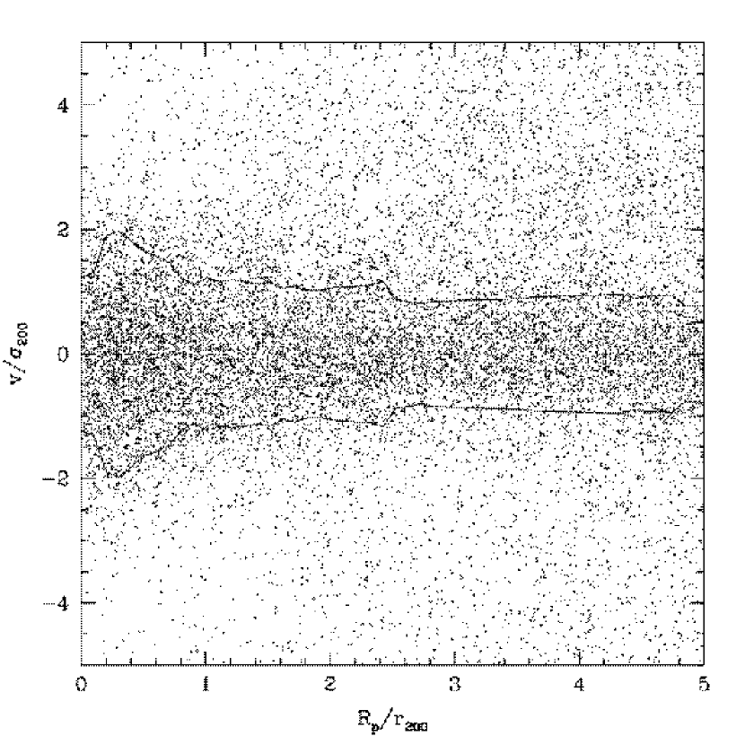
Figure 15: Redshift versus radius for galaxies around the CAIRNS ensemble cluster.

Figure 15 shows the caustic diagrams for the ensemble cluster. The ensemble cluster contains 15103 members within the caustics; 4502 of these are projected within $r_{200}$ and 10,601 have projected radii between 1 and 5 $r_{200}$ (5$r_{200}$ is comparable to the turnaround radii in Table 3). These results confirm that infall regions contain more galaxies than their parent virial regions (Rines et al., 2003, 2004). The ensemble CIRS cluster contains more galaxies both within and outside $r_{200}$ than any previous study.

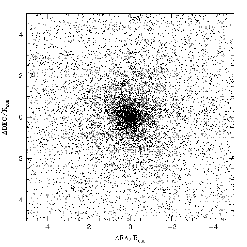
Figure 16: Sky distribution of the ensemble CIRS cluster after removing galaxies near Virgo and NGC4636.

Figure 16 shows the sky distribution of the ensemble cluster members. We remove galaxies near Virgo and NGC4636 for this figure because including them produces non-physical features from the survey pattern. Its appearance is reminiscent of globular clusters and shows that a sufficiently densely sampled ensemble cluster is close to circularly symmetric.

4 Comments on Individual Clusters

Clusters share many common features, but any large sample of clusters contains some complex systems. We comment on some of the most exceptional cases here.

• A119 This cluster is in the CAIRNS survey. See Rines et al. (2003) for discussion. The mass profile computed here is based only on SDSS DR4 data which cover only a limited fraction of the infall region of A119. Despite this difference, the mass profiles from CIRS and CAIRNS agree reasonably well.

• A168 This cluster is in the CAIRNS survey. See Rines et al. (2003) for discussion.

• NGC 5846/NGC 5813 This group is one of the closest X-ray groups. It has been studied extensively, most recently by Mahdavi et al. (2005), who present a velocity dispersion map. This map shows the infall pattern without azimuthal averaging (see their Figure 8). NGC 5846 is the dominant member of the group, and NGC 5813 is the center of a merging subgroup. Despite this ongoing merger, the velocity field on larger scales shows an infall pattern. This group demonstrates that infall patterns can exist in very low-mass systems.

• A1035 This cluster apparently consists of two systems offset by $\sim$3000 ${\rm km~{}s}^{-1}$ in redshift and nearly concentric on the sky. There appears to be two infall patterns which overlap at small radii. From the hierarchical analysis, the components A and B have redshifts $z=0.06748$ and $z=0.08008$ respectively. Component A is $\sim$10^′ SE of component B. In the RASS image, A1035 is elongated NW-SE with a peak in the NW (see Figure 2b of Ledlow et al., 2003). This morphology is confirmed by a 4617 second ROSAT PSPC observation centered 47^′ SE of A1035. Our suggested interpretation is that A1035A and A1035B are both X-ray clusters separated by $\sim$10^′ and that the more distant A1035B contributes most of the X-ray flux. This picture is confirmed by comparing the RASS image to the SDSS image. There are two concentrations of galaxies, one centered roughly on the NW X-ray peak and one centered in the SE extension. The brightest several galaxies in these concentrations confirm that the NW peak is associated with the higher redshift component and the SE extension with the lower redshift component. From the RASS image, A1035B contributes $\sim$2/3 of the total flux, so we estimate $L_{X,A}=7\times 10^{42}$erg s^-1 and $L_{X,B}=2\times 10^{43}$erg s^-1. If these clusters had been cleanly resolved by the catalogs, neither would lie above our flux limit.

• A1173/A1190 These two clusters are separated by 3.4$h^{-1}{\rm Mpc}$ in the plane of the sky and by $\lesssim$500 ${\rm km~{}s}^{-1}$ in redshift, they are likely bound. A1190 is about twice as luminous as A1173 in X-rays. This system is likely a bound binary cluster.

• A1291 This cluster, like A1035A/B, apparently consists of two systems offset by $\sim$2000 ${\rm km~{}s}^{-1}$ in redshift and nearly concentric on the sky (separation $<$4^′). The caustic diagram shows two infall patterns which overlap at small radii. In addition, A1318 (not in CIRS) lies $\sim$4$h^{-1}{\rm Mpc}$ (in projection) from A1291A/B at approximately the same redshift as the higher-redshift cluster. Unlike A1035, A1291 does not contain multiple components in the RASS image. The peak of the RASS extended source is approximately centered on a bright galaxy ($M_{r}\approx$-21.3) in the lower-redshift component. It is not clear whether there is any X-ray emission associated with the higher redshift component. The total flux is 4.2$\times$10^-12erg s^-1cm^-2, so at most one of the two components would meet our flux limit if they were resolved.

• A1728 This cluster has a large offset of 1.3$h^{-1}{\rm Mpc}$ between the X-ray and hierarchical centers. The sky distribution of galaxies reveals two components, one centered roughly on the X-ray peak and the other 1.3$h^{-1}{\rm Mpc}$ WSW which is the hierarchical center (the hierarchical center is $\sim$10’ away from the NED center of ZwCl1320.4+1121, a cluster without a known redshift). A caustic plot centered on the X-ray peak shows an infall pattern with slightly smaller amplitude and a “spike” at the radius of the WSW concentration (similar spikes at the radii of X-ray groups are seen in A2199; see Rines et al., 2002). The RASS image shows no obvious X-ray emission from the WSW concentration. If we apply the caustic technique to the pattern centered on the X-ray peak, the total mass is smaller by about a factor of two.

• A1750A/B As noted in $\S$2.2, the X-ray emission of A1750 has a secondary component to the south of the central emission. These components are separated by 340$h^{-1}{\rm kpc}$ in projection and $\sim$1300 ${\rm km~{}s}^{-1}$ in radial velocity (Belsole et al., 2004). The hierarchical center is located close to the primary X-ray source in both position and redshift.

• A2061/A2067 These two clusters are separated by 1.8$h^{-1}{\rm Mpc}$ in the plane of the sky and by $\sim$600 ${\rm km~{}s}^{-1}$ in redshift, they are likely bound. A2061 is about four times more luminous in X-rays than A2067, so this system is similar to the A2199 supercluster, i.e., a central, massive cluster with an infalling group. These clusters are part of the Cor Bor supercluster (Small et al., 1998; Marini et al., 2004). A2061 contains an X-ray ’plume’ extending in the direction of A2067, suggesting a dynamical connection between the two systems (Marini et al., 2004). The A2069 supercluster (not in CIRS) lies behind both A2067 and A2061 (Postman et al., 1988; Small et al., 1998). It is possible that hot gas in condensed substructures in the A2069 supercluster contribute to the measured X-ray flux attributed to A2067 and/or A2061.

• A2149 This cluster has two components along the line of sight, one at $z$=0.0675 and one at $z$=0.1068. The former redshift is adopted by eBCS and the latter redshift is adopted by NORAS. A close inspection of the RASS image for this cluster shows an extended area of X-ray emission peaked on the BCG of the $z$=0.0675 component. We conclude that most of the X-ray flux comes from the system at lower redshift with possible contamination from the more distant system.

• A2197/A2199 This cluster is in the CAIRNS survey. See Rines et al. (2001, 2002) for discussion. A2197 has a 750$h^{-1}{\rm kpc}$ offset between the X-ray and hierarchical centers. A2197 is composed of two X-ray groups, A2197W and A2197E. The X-ray center is the peak of A2197W; the hierarchical center is located approximately midway between A2197W and A2197E.

• A2244/A2245/A2249 These three clusters are in a fairly small volume of the universe. A2245 ($z$=0.086) is the most massive of the three, followed by A2244 ($z$=0.0997) $\sim$30^′north. A2249 ($z$=0.086) is centered about 2 degrees east and just off the edge of the SDSS spectroscopic survey. In addition, there’s a loose system (A2241B, in the background of A2241) SW of A2245 which is at $z$$\sim$0.097 but seems to have multiple components along the line of sight.

5 Comparison to Virial and Projected Mass Estimates

Zwicky (1933, 1937) first used the virial theorem to estimate the mass of the Coma cluster. With some modifications, notably a correction term for the surface pressure (The & White, 1986), the virial theorem remains in wide use (e.g., Girardi et al., 1998, and references therein). Jeans analysis incorporates the radial dependence of the projected velocity dispersion (e.g., Carlberg et al., 1997; van der Marel et al., 2000; Biviano & Girardi, 2003, and references therein) and obviates the need for a surface term.

Jeans analysis and the caustic method are closely related. Both use the phase space distribution of galaxies to estimate the cluster mass profile. The primary difference is that the Jeans method assumes that the cluster is in dynamical equilibrium; the caustic method does not. The Jeans method depends on the width of the velocity distribution of cluster members at a given radius, whereas the caustic method calculates the edges of the velocity distribution at a given radius. The caustic method is not independent of the Jeans method, as the D99 method minimizes $|<$$v_{esc}^{2}$$>_{R}-4<$$v^{2}$$>_{R}|$ within the virial region with radius R (see D99 for a more detailed discussion). Mass estimates based on Jeans analysis thus provide a consistency check but not an independent verification of the caustic mass estimates.

Applying the Jeans method requires an assumption about either the mass distribution or the orbital distribution. Typically, one assumes that light traces mass and thus that the projected galaxy density is proportional to the projected mass density (e.g., Girardi et al., 1998) or one assumes a functional form for the orbital distribution (e.g., Biviano & Girardi, 2003). Note that most authors make the implicit assumption that the orbital distribution of the dark matter can be inferred from that of the galaxies. Many recent simulations suggest that little ($\sim$10%) or no velocity bias exists on linear and mildly non-linear scales (Kauffmann et al., 1999a, b; Diemand et al., 2004; Faltenbacher et al., 2005). However, galaxies in simulated clusters often have significantly different orbital distributions than the dark matter (e.g., Klypin et al., 1999; Koranyi, 2000; Faltenbacher et al., 2005). Dynamical friction should produce a smaller velocity dispersion for cluster galaxies than dark matter (Klypin et al., 1999; Yoshikawa et al., 2003; van den Bosch et al., 2005), although they may undergo more frequent mergers (due to their smaller velocities) or tidal disruption, resulting in a larger velocity dispersion of the surviving cluster galaxies relative to the dark matter (Colín et al., 1999; Diemand et al., 2004; Faltenbacher et al., 2005). Note also that velocity bias may depend on the mass of the cluster (Berlind et al., 2003) or the luminosities of the tracer galaxies (Slosar et al., 2006). An important caveat is that the subhalo distribution of cluster galaxies in simulations does not match the observed distributions of cluster galaxies: real cluster galaxies trace the dark matter profile, while simulated cluster galaxies are significantly antibiased in cluster centers, likely due to the resilience of the stellar component of a subhalo against tidal disruption relative to the total subhalo (e.g., Diemand et al., 2004; Faltenbacher et al., 2006). The details of velocity bias depend also on the selection used to identify subhaloes, e.g., whether subhalo mass is measured prior to or after a subhalo enters the cluster (Faltenbacher et al., 2006). The amount of velocity bias in simulations is typically $\sim$10% for cluster-size haloes, although disagreement remains on whether this bias is positive or negative. Velocity bias of this size would lead to virial masses overestimated or underestimated by $\sim$20%. Future work is clearly needed to understand the nature and significance of velocity bias for cluster mass estimates. There is no clear evidence from observations in favor of or against velocity bias in clusters, although the generally good agreement between X-ray, lensing, and virial mass estimates suggests that any velocity bias is not large ($\lesssim$20%; e.g., Girardi et al., 1998; Popesso et al., 2004; Diaferio et al., 2005). Because significant velocity bias would produce incorrect virial mass estimates, the agreement between virial and caustic mass estimates is no guarantee that the caustic mass estimates are accurate. However, the mechanisms which cause velocity bias are less effective in the outskirts of clusters, so the caustic technique should be less affected by velocity bias than estimates based on Jeans’ analysis. Analysis of simulations of large-scale structure with very large dynamic range (Springel et al., 2005) or of individual clusters (Borgani et al., 2006) may provide a clearer understanding of the potential impact of velocity bias on cluster mass estimates from galaxy kinematics.

Another common assumption is that the kinematics of galaxies are independent of their luminosities. The consistency of CAIRNS mass profiles and velocity dispersion profiles for $K_{s}$-band luminosity-limited and deeper samples indicates that this is a reasonable approximation (Rines et al., 2004), but theoretical models of subhaloes suggest that velocity bias should depend on luminosity (Slosar et al., 2006). We plan to use the CIRS sample to test this assumption in future work by studying the luminosity dependence of the kinematic distribution of galaxies. Note that the CIRS clusters are sampled to depths of $\sim$$M^{*}$+1 for the most distant clusters to $\sim$$M^{*}$+7 for Virgo, so the CIRS caustics sample a wide range of luminosity limits. We confirm that the ratio of virial to caustic mass estimates in an X-ray luminosity-limited sample shows no significant trend with redshift, indicating that the different spectroscopic sampling limits do not affect these comparisons. Similarly, the ratio of caustic masses to X-ray luminosities is not significantly different for an X-ray luminosity-limited sample. These results suggest that any velocity bias does not depend strongly on galaxy luminosity. We defer further discussion to future work.

We apply the virial mass and projected mass estimators (Heisler et al., 1985) to the CIRS clusters. For the latter, we assume the galaxies are on isotropic orbits. We must define a radius of virialization within which the galaxies are relaxed. We use $r_{200}$ (Table 3) and include only galaxies within the caustics. We thus assume that the caustics provide a good division between cluster galaxies and interlopers (see Figures 2-7).

We calculate the virial mass according to

$$M_{vir}=\frac{3\pi}{2}\frac{\sigma_{p}^{2}R_{PV}}{G}$$ (5)

where $R_{PV}=2N(N-1)/\sum_{i,j>i}R_{ij}^{-1}$ is the projected virial radius and $\sigma_{p}^{2}=\sum_{i}(v_{i}-\bar{v})^{2}/(N-1)$. If the system does not lie entirely within $r_{200}$, a surface pressure term 3PV should be added to the usual virial theorem so that $2T+U=3PV$. The virial mass is then an overestimate of the mass within $r_{200}$ by the fractional amount

$$C=4\pi r_{200}^{3}\frac{\rho(r_{200})}{\int_{0}^{r_{200}}4\pi r^{2}\rho dr}\Bigg{[}{\frac{\sigma_{r}(r_{200})}{\sigma(<r_{200})}\Bigg{]}^{2}}$$ (6)

where $\sigma_{r}(r_{200})$ is the radial velocity dispersion at $r_{200}$ and $\sigma(<r_{200})$ is the enclosed total velocity dispersion within $r_{200}$ (e.g., Girardi et al., 1998). In the limiting cases of circular, isotropic, and radial orbits, the maximum value of the term involving the velocity dispersion is 0, 1/3, and 1 respectively.

The projected mass estimator is more robust in the presence of close pairs. The projected mass is

$$M_{proj}=\frac{32}{\pi G}\sum_{i}{R_{i}(v_{i}-v)^{2}}/N$$ (7)

where we assume isotropic orbits and a continuous mass distribution. If the orbits are purely radial or purely circular, the factor 32 becomes 64 or 16 respectively. We estimate the uncertainties using the limiting fractional uncertainties $\pi^{-1}(2\mbox{ln}N)^{1/2}N^{-1/2}$ for the virial theorem and $\approx 1.4N^{-1/2}$ for the projected mass. These uncertainties do not include systematic uncertainties due to membership determination or the assumption of isotropic orbits in the projected mass estimator. Table 6 lists the virial and projected mass estimates.

Figure 17 compare the virial and caustic mass estimates at $r_{200}$. The mean ratios of these estimates are $M_{c}/M_{v}=1.01\pm 0.04$. The caustic mass estimates are consistent with virial mass estimates even assuming a correction factor $C\approx 0.1-0.2M_{vir}$, consistent with the best-fit NFW profiles (see also Carlberg et al., 1997; Girardi et al., 1998; Koranyi & Geller, 2000; Rines et al., 2003).

Figures 18-23 compare the mass profiles estimated from the caustics, virial theorem, and projected mass estimator. In the caustic technique, errors on the mass profiles are estimated by the inverse of the peak of the galaxy number density in the redshift diagrams. The errors derived with this recipe agree with the typical spread of mass profiles measured in simulated clusters (D99, Diaferio et al 2006, in prep). The projected mass estimator consistently overestimates the mass at small radii and underestimates the mass at large radii relative to the other profiles. This behavior suggests that this estimator is best for estimating virial masses but not mass profiles. The virial and caustic mass profiles generally agree although there are many clusters with large disagreements. The caustic mass profiles do not appear to consistently overestimate or underestimate the mass relative to the virial mass profiles. This result supports our use of caustic mass profiles as a tracer of the total cluster mass profile ($\S$3.5).

6 Velocity Dispersion Profiles

Several authors have explored the use of the velocity dispersion profile (VDP) of clusters as a diagnostic of their dynamical states. For example, Fadda et al. (1996) find that VDPs typically have three shapes: increasing, flat, or decreasing with radius.

We calculate the VDPs of the CIRS clusters using all galaxies inside the caustics. Most of the CIRS clusters display decreasing VDPs within about $r_{200}$ (Figure 24 displays the first 12 clusters in RA). The VDPs either flatten out or continue to decrease between $r_{200}$ and $r_{t}$, consistent with the results of CAIRNS.

Some authors (Carlberg et al., 1997; Girardi et al., 1998) suggest that an accurate estimate of $r_{200}$ can be obtained for a cluster from the asymptotic value of the enclosed velocity dispersion $\sigma_{p}(<r)$ calculated for all galaxies within a given radius. Many of the CIRS clusters, however, display no obvious convergence in the enclosed velocity dispersion (shown by dashed lines in Figure 24). If the rich clusters in the CNOC1 survey are similar to their CIRS cousins, the use of the asymptotic value of the enclosed velocity dispersion to estimate $r_{200}$ may be unreliable. The caustic technique provides an alternative method for estimating $r_{200}$, although applying it requires many more redshifts than are needed for computing the velocity dispersion.

7 Summary

We use the Fourth Data Release of the Sloan Digital Sky Survey to test the ubiquity of infall patterns around galaxy clusters. The CAIRNS project found infall patterns in all 9 clusters in the survey, but the cluster sample was small and incomplete. Matching X-ray cluster catalogs with SDSS, we search for infall patterns in a complete sample of 72 X-ray selected clusters. Well-defined infall patterns are apparent in most of the clusters, with the fraction decreasing with increasing redshift due to shallower sampling. All clusters in a well-defined sample limited by redshift (ensuring good sampling) and X-ray flux (excluding superpositions) show infall patterns sufficient for calculating caustic mass profiles. Similar to CAIRNS, cluster infall patterns are better defined in observations than in simulations. Further work is needed to determine whether this difference lies in the galaxy formation recipes used in simulations or is more fundamental.

We use the infall patterns to compute mass profiles for the clusters and compare them to model profiles. We confirm the conclusion of CAIRNS that cluster infall regions are well fit by NFW and Hernquist profiles and poorly fit by singular isothermal spheres. Observed clusters resemble those in simulations, and their mass profiles are well described by extrapolations of NFW or Hernquist models out to the turnaround radius. The scaled mass profiles indicate that NFW profiles are favored over Hernquist and SIS profiles. The shapes of the best-fit NFW cluster mass profiles agree reasonably well with the predictions of simulations; the average mass profile has $c_{200}$$\approx$7.2, slightly larger than the value for cluster size halos extrapolated from Bullock et al. (2001) and with similar scatter. These mass profiles test the shapes of dark matter haloes on a scale difficult to probe with weak lensing or any other mass estimator. The caustic pattern is often visible up to and beyond the turnaround radius. The mass within the turnaround radius (for clusters where the radial extent of the caustics $r_{max}$ exceeds the turnaround radius) is 2.19$\pm$0.18 times the virial mass $M_{200}$ (the average ratio for all clusters is 1.97$\pm$0.10), in agreement with the numerical simulations of $\Lambda$CDM clusters of Busha et al. (2005), who find that the final mass of cluster scale halos in the far future is 1.9 times larger than $M_{200}$ measured at the present epoch.

We stack the clusters to produce an ensemble cluster containing 4502 galaxies projected within $r_{200}$ and an additional 10,601 within 5$r_{200}$ (roughly the turnaround radius). The infall region thus contains more galaxies than the virial region. The ensemble cluster appears circularly symmetric.

At small radii, the caustic mass profiles are consistent with independent X-ray mass estimates using previously determined scaling relations such as those found for RASS-SDSS (Popesso et al., 2005). This good agreement indicates that the caustic technique is a reliable mass estimator (see also Rines et al., 2003). At larger radii, the caustic masses agree well with virial masses.

The CAIRNS project demonstrated that the caustic pattern is common in rich, X-ray luminous galaxy clusters. The CIRS sample, eight times larger than the CAIRNS sample, confirms and extends many of the results of CAIRNS. Future papers in the CIRS project will analyze the relative distributions of mass and light in cluster infall regions, X-ray and optical substructure within infall regions, and the dependence of galaxy properties on environment.

Figure 1: Redshift versus X-ray luminosity (0.1-2.4 keV) for X-ray clusters from XBACS, BCS/eBCS, NORAS, and REFLEX contained in the SDSS DR4 spectroscopic survey region. Filled squares, open squares and crosses indicate clusters with “clean” infall patterns, “intermediate” infall patterns, and no obvious infall pattern respectively. The X-ray cluster catalogs are complete to approximately $f_{X}>$3$\times$10^-12erg s^-1 (curved line). The solid line shows the flux and redshift limits of the CIRS cluster sample. The dash-dotted line shows the redshift and luminosity limits of CAIRNS.

Figure 8: Velocity dispersions at $r_{200}$ compared to X-ray luminosities. The solid line is the bisector of the least squares fits. The dashed lines show the $\sigma_{200}-L_{X}$ relations from RASS-SDSS (Popesso et al., 2005).

Figure 10: X-ray temperatures versus caustic masses at $r_{200}$. The solid line is the bisector of the ordinary least squares fits. The dashed and dash-dotted lines are the relations found by Popesso et al. (2005) and Finoguenov et al. (2001) respectively.

Figure 11: Caustic masses at $r_{200}$ compared to velocity dispersions within $r_{200}$. The solid line is the bisector of the ordinary least squares fits.

Figure 13: Concentrations $c_{101}$=$r_{101}/a$ of the best-fit NFW profiles verus $M_{101}$. The heavy dashed line shows the expected trend from simulations and the thin dashed line shows a model of this trend, while the errorbars show the expected $1\sigma$ scatter in $c_{101}$ (Bullock et al., 2001). The stars and triangles show the mean and median values of $\mbox{log}(c_{101})$ in six bins of 12 clusters. The thin errorbars show the $1\sigma$ scatter in the mean values of $\mbox{log}(c_{101})$ in each bin.

Figure 14: Ratio of maximum mass $M_{max}$ to virial mass $M_{200}$ versus maximum radius $R_{max}$. Squares are clusters where $r_{t}<r_{max}$, triangles are clusters with $r_{t}\geq r_{max}$. Solid points indicate clusters with $M_{200}\geq$3$\times$10${}^{14}h^{-1}M_{\odot}$. Crosses are the CAIRNS clusters. The two lines indicate the simulations of Tinker et al. (2005) for massive clusters for $\Omega_{m}=0.1$ and 0.45.

Figure 17: Caustic masses at $r_{200}$ compared to virial masses at the same radius. Errorbars show 1$\sigma$ uncertainties and the solid line has slope unity.

Figure 24: Velocity dispersion profiles for the CIRS clusters. The solid lines show the velocity dispersion profile of member galaxies (those within the caustics) in a moving bin of 25 galaxies. Errorbars indicate 1-$\sigma$ uncertainties for independent bins. The dashed lines show the enclosed velocity dispersion profiles. Vertical lines indicate $r_{200}$ and $r_{t}$. The axes are identical in all panels.

Table 1: CIRS Basic Properties

Cluster	X-ray Coordinates		$z_{\odot}$	$L_{X}/10^{43}$	Catalog	$T_{X}$	$\sigma_{p}$	Flag	$R_{comp}$
	RA (J2000)	DEC (J2000)		erg s-1		keV	${\rm km~{}s}^{-1}$		$h^{-1}{\rm Mpc}$
A0085	10.45880	-9.30190	0.0557	2.805	REF	5.87	$692^{+55}_{-45}$	2	1.8
A0119	14.07620	-1.21670	0.0446	0.781	REF	5.93	$589^{+68}_{-51}$	2	0.1
A0160	18.27410	15.51700	0.0432	0.092	NOR	2.70	$489^{+62}_{-45}$	2	0.7
A0168	18.80000	00.33000	0.0451	0.247	REF	2.60	$577^{+50}_{-40}$	2	2.1
RXJ0137	24.31420	-9.20280	0.0409	0.155	REF	0.00	$392^{+45}_{-34}$	2	2.1

Table 2: CIRS Hierarchical Centers and Offsets

Cluster	Hierarchical Center		$\Delta cz$	$\Delta R$
	RA (J2000)	DEC (J2000)	${\rm km~{}s}^{-1}$	$h^{-1}{\rm kpc}$
A0085	10.42629	-9.42550	-45	347
A0119	14.03449	-1.16356	-106	149
A0160	18.25117	15.49587	285	65
A0168	18.81422	00.26408	-17	150
RXJ0137	24.35443	-9.27309	-12	164

Table 3: CIRS Characteristic Radii and Masses

Cluster	$r_{500}$	$r_{200}$	$r_{t}$	$r_{max}$	$M_{200}$	$M_{t}$	$M_{max}/M_{200}$
	$h^{-1}{\rm Mpc}$	$h^{-1}{\rm Mpc}$	$h^{-1}{\rm Mpc}$	$h^{-1}{\rm Mpc}$	$10^{14}M_{\odot}$	$10^{14}M_{\odot}$
A0085	0.67	1.02	4.99	4.34	2.50$\pm$ 1.19	5.04$\pm$2.95	2.02
A0119	0.60	0.91	4.69	3.64	1.77$\pm$ 0.70	4.19$\pm$1.88	2.37
A0160	0.46	0.67	2.70	1.31	0.68$\pm$ 0.38	0.80$\pm$0.54	1.17
A0168	0.63	0.95	4.19	3.94	2.02$\pm$ 0.51	3.00$\pm$0.93	1.48
RXJ0137	0.46	0.72	3.14	2.42	0.87$\pm$ 0.06	1.26$\pm$0.09	1.45

Table 4: Individual Limits for CIRS Clusters

Cluster	$R_{p}$	$\Delta cz$
	$h^{-1}{\rm Mpc}$	${\rm km~{}s}^{-1}$
A160	–	$-1500\rightarrow+3000$
RXJ0137	5	$-5000\rightarrow+3000$
A954	5	–
A1035B	–	$+1500\rightarrow+7000$
A1173	3	–
A1291A	5	$-5000\rightarrow-1000$
A1377	5	$-5000\rightarrow+2000$
A1436	6	–
RXJ1210	4	–
NGC4325	1.5	–
NGC4636	1.0	$\pm$2000
RXJ1351	3	–
MS1306	5	–
NGC5846	5	–
A2067	1.5	–
A2149	4	–
NGC6107	4	–
A2197	1.5	–
A2245	–	$-5000\rightarrow+3000$
A2244	1.5	$-3000\rightarrow+5000$
A2249	6	$\pm 4000$

Table 5: CIRS Mass Profile Fit Parameters

Cluster	$a_{NFW}$	$r_{200}$	$c_{NFW}$	$M_{200}$	Best-fit	$c_{101}$
	$h^{-1}{\rm Mpc}$	$h^{-1}{\rm Mpc}$		$10^{14}M_{\odot}$	Profile
A85	0.223	1.00	4.50	2.35	H	6.07
A119	0.350	0.89	2.55	1.65	H	3.52
A160	0.064	0.65	10.14	0.64	H	13.36
A168	0.114	0.88	7.69	1.57	H	10.20
RXJ0137	0.105	0.67	6.34	0.69	H	8.45

Table 6: CIRS Virial and Projected Masses

Cluster	$r_{200}$	$M_{200}$	$M_{proj}$	$M_{vir}$
	$h^{-1}{\rm Mpc}$	$10^{14}M_{\odot}$	$10^{14}M_{\odot}$	$10^{14}M_{\odot}$
A0085	1.02	2.50$\pm$ 1.19	2.11$\pm$0.30	2.94$\pm$0.29
A0119	0.91	1.77$\pm$ 0.70	1.68$\pm$0.33	1.33$\pm$0.17
A0160	0.67	0.68$\pm$ 0.38	0.56$\pm$0.12	1.17$\pm$0.15
A0168	0.95	2.02$\pm$ 0.51	1.49$\pm$0.23	2.02$\pm$0.21
RXJ0137	0.72	0.87$\pm$ 0.06	0.63$\pm$0.12	0.84$\pm$0.10

References

- Adelman-McCarthy et al. (2006) Adelman-McCarthy, J. et al. 2006, ApJS, 162, 38
- Böhringer et al. (2000a) Böhringer, H. et al. 2000a, ApJS, 129, 435
- Böhringer et al. (2000b) —. 2000b, ApJS, 129, 435
- Böhringer et al. (2001) —. 2001, A&A, 369, 826
- Böhringer et al. (2004) —. 2004, A&A, 425, 367
- Belsole et al. (2004) Belsole, E., Pratt, G. W., Sauvageot, J.-L., & Bourdin, H. 2004, A&A, 415, 821
- Berlind et al. (2003) Berlind, A. A. et al. 2003, ApJ, 593, 1
- Biviano & Girardi (2003) Biviano, A. & Girardi, M. 2003, ApJ, 585, 205
- Blanton et al. (2003) Blanton, M. R. et al. 2003, ApJ, 592, 819
- Borgani et al. (2004) Borgani, S. et al. 2004, MNRAS, 348, 1078
- Borgani et al. (2006) —. 2006, MNRAS, 270
- Broadhurst et al. (2005a) Broadhurst, T., Takada, M., Umetsu, K., Kong, X., Arimoto, N., Chiba, M., & Futamase, T. 2005a, ApJ, 619, L143
- Broadhurst et al. (2005b) Broadhurst, T. et al. 2005b, ApJ, 621, 53
- Bullock et al. (2001) Bullock, J. S. et al. 2001, MNRAS, 321, 559
- Busha et al. (2003) Busha, M. T., Adams, F. C., Wechsler, R. H., & Evrard, A. E. 2003, ApJ, 596, 713
- Busha et al. (2005) Busha, M. T., Evrard, A. E., Adams, F. C., & Wechsler, R. H. 2005, MNRAS, 363, L11
- Carlberg et al. (1997) Carlberg, R. G., Yee, H. K. C., & Ellingson, E. 1997, ApJ, 478, 462
- Cavaliere & Fusco-Femiano (1976) Cavaliere, A. & Fusco-Femiano, R. 1976, A&A, 49, 137
- Clowe & Schneider (2001) Clowe, D. & Schneider, P. 2001, A&A, 379, 384
- Colín et al. (1999) Colín, P., Klypin, A. A., Kravtsov, A. V., & Khokhlov, A. M. 1999, ApJ, 523, 32
- Cross et al. (2004) Cross, N. J. G., Driver, S. P., Liske, J., Lemon, D. J., Peacock, J. A., Cole, S., Norberg, P., & Sutherland, W. J. 2004, MNRAS, 349, 576
- Danese et al. (1980) Danese, L., de Zotti, G., & di Tullio, G. 1980, A&A, 82, 322
- David et al. (1993) David, L. P., Slyz, A., Jones, C., Forman, W., Vrtilek, S. D., & Arnaud, K. A. 1993, ApJ, 412, 479
- Diaferio (1999) Diaferio, A. 1999, MNRAS, 309, 610
- Diaferio & Geller (1997) Diaferio, A. & Geller, M. J. 1997, ApJ, 481, 633
- Diaferio et al. (2005) Diaferio, A., Geller, M. J., & Rines, K. J. 2005, ApJ, 628, L97
- Diemand et al. (2004) Diemand, J., Moore, B., & Stadel, J. 2004, MNRAS, 352, 535
- Drinkwater et al. (2001) Drinkwater, M. J., Gregg, M. D., & Colless, M. 2001, ApJ, 548, L139
- Ebeling et al. (2000a) Ebeling, H., Edge, A. C., Allen, S. W., Crawford, C. S., Fabian, A. C., & Huchra, J. P. 2000a, MNRAS, 318, 333
- Ebeling et al. (2000b) —. 2000b, MNRAS, 318, 333
- Ebeling et al. (1996) Ebeling, H., Voges, W., Bohringer, H., Edge, A. C., Huchra, J. P., & Briel, U. G. 1996, MNRAS, 281, 799
- Eke et al. (1996) Eke, V. R., Cole, S., & Frenk, C. S. 1996, MNRAS, 282, 263
- Ellingson et al. (2001) Ellingson, E., Lin, H., Yee, H. K. C., & Carlberg, R. G. 2001, ApJ, 547, 609
- Evrard et al. (1996) Evrard, A. E., Metzler, C. A., & Navarro, J. F. 1996, ApJ, 469, 494
- Fadda et al. (1996) Fadda, D., Girardi, M., Giuricin, G., Mardirossian, F., & Mezzetti, M. 1996, ApJ, 473, 670
- Faltenbacher et al. (2005) Faltenbacher, A., Kravtsov, A. V., Nagai, D., & Gottlöber, S. 2005, MNRAS, 358, 139
- Faltenbacher et al. (2006) —. 2006, MNRAS, submitted (astro-ph/0602197)
- Finoguenov et al. (2001) Finoguenov, A., Reiprich, T. H., & Böhringer, H. 2001, A&A, 368, 749
- Gavazzi (2005) Gavazzi, R. 2005, A&A, 443, 793
- Geller et al. (1999) Geller, M. J., Diaferio, A., & Kurtz, M. J. 1999, ApJ, 517, L23
- Girardi et al. (1998) Girardi, M., Giuricin, G., Mardirossian, F., Mezzetti, M., & Boschin, W. 1998, ApJ, 505, 74
- Gramann & Suhhonenko (2002) Gramann, M. & Suhhonenko, I. 2002, MNRAS, 337, 1417
- Heisler et al. (1985) Heisler, J., Tremaine, S., & Bahcall, J. N. 1985, ApJ, 298, 8
- Hernquist (1990) Hernquist, L. 1990, ApJ, 356, 359
- Horner (2001) Horner, D. 2001, Ph.D. Thesis, University of Maryland
- Horner et al. (1999) Horner, D. J., Mushotzky, R. F., & Scharf, C. A. 1999, ApJ, 520, 78
- Jones & Forman (1999) Jones, C. & Forman, W. 1999, ApJ, 511, 65
- Kaiser (1987) Kaiser, N. 1987, MNRAS, 227, 1
- Kauffmann et al. (1999a) Kauffmann, G., Colberg, J. M., Diaferio, A., & White, S. D. M. 1999a, MNRAS, 303, 188
- Kauffmann et al. (1999b) —. 1999b, MNRAS, 307, 529
- Klypin et al. (1999) Klypin, A., Gottlöber, S., Kravtsov, A. V., & Khokhlov, A. M. 1999, ApJ, 516, 530
- Kneib et al. (2003) Kneib, J.-P. et al. 2003, ApJ, 598, 804
- Koranyi (2000) Koranyi, D. M. 2000, Ph.D. Thesis, Harvard University
- Koranyi & Geller (2000) Koranyi, D. M. & Geller, M. J. 2000, AJ, 119, 44
- Lahav et al. (1991) Lahav, O., Rees, M. J., Lilje, P. B., & Primack, J. R. 1991, MNRAS, 251, 128
- Ledlow et al. (2003) Ledlow, M. J., Voges, W., Owen, F. N., & Burns, J. O. 2003, AJ, 126, 2740
- Lin et al. (2004) Lin, Y., Mohr, J. J., & Stanford, S. A. 2004, ApJ, 610, 745
- Łokas & Mamon (2003) Łokas, E. L. & Mamon, G. A. 2003, MNRAS, 343, 401
- Mahdavi et al. (1999) Mahdavi, A., Geller, M. J., Böhringer, H., Kurtz, M. J., & Ramella, M. 1999, ApJ, 518, 69
- Mahdavi et al. (2005) Mahdavi, A., Trentham, N., & Tully, R. B. 2005, AJ, 130, 1502
- Majumdar & Mohr (2004) Majumdar, S. & Mohr, J. J. 2004, ApJ, 613, 41
- Marini et al. (2004) Marini, F. et al. 2004, MNRAS, 353, 1219
- Miller et al. (2005) Miller, C. J. et al. 2005, AJ, 130, 968
- Moore et al. (1999) Moore, B., Quinn, T., Governato, F., Stadel, J., & Lake, G. 1999, MNRAS, 310, 1147
- Nagamine & Loeb (2003) Nagamine, K. & Loeb, A. 2003, New Astronomy, 8, 439
- Navarro et al. (1997) Navarro, J. F., Frenk, C. S., & White, S. D. M. 1997, ApJ, 490, 493
- Nevalainen et al. (2000) Nevalainen, J., Markevitch, M., & Forman, W. 2000, ApJ, 532, 694
- Plaga (2005) Plaga, R. 2005, A&A, 440, L41
- Popesso et al. (2005) Popesso, P., Biviano, A., Böhringer, H., Romaniello, M., & Voges, W. 2005, A&A, 433, 431
- Popesso et al. (2004) Popesso, P., Böhringer, H., Brinkmann, J., Voges, W., & York, D. G. 2004, A&A, 423, 449
- Postman et al. (1988) Postman, M., Geller, M. J., & Huchra, J. P. 1988, AJ, 95, 267
- Regös & Geller (1989) Regös, E. & Geller, M. J. 1989, AJ, 98, 755
- Reisenegger et al. (2000) Reisenegger, A., Quintana, H., Carrasco, E. R., & Maze, J. 2000, AJ, 120, 523
- Rines et al. (2004) Rines, K., Geller, M. J., Diaferio, A., Kurtz, M. J., & Jarrett, T. H. 2004, AJ, 128, 1078
- Rines et al. (2002) Rines, K., Geller, M. J., Diaferio, A., Mahdavi, A., Mohr, J. J., & Wegner, G. 2002, AJ, 124, 1266
- Rines et al. (2000) Rines, K., Geller, M. J., Diaferio, A., Mohr, J. J., & Wegner, G. A. 2000, AJ, 120, 2338
- Rines et al. (2003) Rines, K., Geller, M. J., Kurtz, M. J., & Diaferio, A. 2003, AJ, 126, 2152
- Rines et al. (2005) —. 2005, AJ, 130, 1482
- Rines et al. (2001) Rines, K., Mahdavi, A., Geller, M. J., Diaferio, A., Mohr, J. J., & Wegner, G. 2001, ApJ, 555, 558
- Slosar et al. (2006) Slosar, A., Seljak, U., & Tasitsiomi, A. 2006, MNRAS, 366, 1455
- Small et al. (1998) Small, T. A., Ma, C., Sargent, W. L. W., & Hamilton, D. 1998, ApJ, 492, 45
- Springel et al. (2005) Springel, V. et al. 2005, Nature, 435, 629
- Stoughton et al. (2002) Stoughton, C. et al. 2002, AJ, 123, 485
- Strauss et al. (2002) Strauss, M. A. et al. 2002, AJ, 124, 1810
- Tegmark et al. (2004) Tegmark, M. et al. 2004, Phys. Rev. D, 69, 103501
- The & White (1986) The, L. S. & White, S. D. M. 1986, AJ, 92, 1248
- Tinker et al. (2005) Tinker, J. L., Weinberg, D. H., Zheng, Z., & Zehavi, I. 2005, ApJ, 631, 41
- van den Bosch et al. (2003) van den Bosch, F. C., Mo, H. J., & Yang, X. 2003, MNRAS, 345, 923
- van den Bosch et al. (2005) van den Bosch, F. C., Weinmann, S. M., Yang, X., Mo, H. J., Li, C., & Jing, Y. P. 2005, MNRAS, 361, 1203
- van der Marel et al. (2000) van der Marel, R. P., Magorrian, J., Carlberg, R. G., Yee, H. K. C., & Ellingson, E. 2000, AJ, 119, 2038
- Vedel & Hartwick (1998) Vedel, H. & Hartwick, F. D. A. 1998, ApJ, 501, 509
- Voges et al. (1999) Voges, W. et al. 1999, A&A, 349, 389
- Yoshikawa et al. (2003) Yoshikawa, K., Jing, Y. P., & Börner, G. 2003, ApJ, 590, 654
- Zwicky (1933) Zwicky, F. 1933, Helv. Phys. Acta, 6, 110
- Zwicky (1937) —. 1937, ApJ, 86, 217