SDSS J143030.22-001115.1: A misclassified narrow-line Seyfert 1 galaxy with flat X-ray spectrum

Abstract

We used multi-component profiles to model H$\beta$ and [O III]$\lambda\lambda$4959,5007 lines for SDSS J143030.22-001115.1, a narrow-line Seyfert 1 galaxy (NLS1) in a sample of 150 NLS1s candidates selected from the Sloan Digital Sky Survey (SDSS) Early Data Release (EDR). After subtracting the H$\beta$ contribution from narrow line regions (NLRs), we found that its full width half maximum (FWHM) of broad H$\beta$ line is nearly 2900 km s^-1, significantly larger than the customarily adopted criterion of 2000 km s^-1. With its weak Fe II multiples, we think that SDSS J143030.22-001115.1 can’t be classified as a genuine NLS1. When we calculate the virial black hole masses of NLS1s, we should use the H$\beta$ linewidth after subtracting the H$\beta$ contribution from NLRs.

1 Introduction

Narrow-line Seyfert 1 galaxies (NLS1s) were defined by their optical spectral characteristics: H$\beta$ full width half maximum(FWHM) less than 2000 km s^-1; strong optical FeII multiples; the line-intensity ratio of [O III]$\lambda 5007$ to H$\beta$ less than 3 (Osterbrock & Pogge 1985; Goodrich 1998). These properties suggested that NLS1s likely contain less massive black holes with higher Eddington ratios (Pounds et al. 1995; Wandel & Boller (1998); Laor et al. 1997; Mineshige et al. 2000), putting NLS1s at one extreme end of the so-called Boroson & Green (1992) eigenvector 1. Their locus in the $M-\sigma$ relation plane is possible special relative to the other AGNs(e.g. Bian & Zhao 2004; Grupe & Mathur 2004; Greene & Ho 2005c). X-ray observation of NLS1s revealed a strong X-ray excess and NLS1s generally have softer X-ray spectra than other active galactic nuclei (AGNs) (Boller et al. 1996; Leighly 1999). Grupe et al. (2004) found that ultra-soft X-ray selection method can be used to find large numbers of NLS1s.

Williams et al. (2003) presented a sample of 150 NLS1s candidates found within Sloan Digital Sky Survey (SDSS) Early Data Release (EDR; Stoughton et al. 2002), which is the largest published sample of NLS1s. 17 of these SDSS NLS1s are observed with Chandra and it is suggested ultrasoft X-ray emission is not a universal characteristic of NLS1s (Williams et al. 2004). For two objects with the smallest photon indices, SDSS J125943.59+010255.1 and SDSS J143030.22-001115.1, the photon indices are less than one. For this sample of 150 SDSS NLS1s, we have used multi-component profiles model to carefully analysis the narrow line regions (NLRs) outflow relative to broad line regions (BLRs) (Bian, Yuan & Zhao 2005). For SDSS J143030.22-001115.1, the line-intensity ratio of [O III]$\lambda$5007 to narrow H$\beta$ is the largest, up to 9.6.

In this paper, we presented our multi-component profiles modelling for SDSS J143030.22-001115.1. The spectral analysis method is introduced in Sect. 2. The results of profile fitting are given in Sect. 3. Our discussion is presented in the last section. All of the cosmological calculations in this paper assume $H_{0}=75\rm{~{}km~{}s^{-1}~{}Mpc^{-1}}$, $\Omega_{M}=0.3$, $\Omega_{\Lambda}=0.7$.

2 DATA and ANALYSIS

Using the SDSS Query Tool, Williams et al. (2003) selected objects fron SDSS EDR that were flagged as QSOs and that showed narrow H$\beta$ lines. They then directly measured the width of the line halfway between the fitted continuum and the H$\beta$ line peak as the FWHM(H$\beta$). At last, they obtained a sample of 150 SDSS NLS1s. SDSS J143030.22-001115.1 is one object in this sample and its spectrum is obtained from SDSS Data Release 3 (DR3; Abazajian et al. 2005) (See left panel in Fig. 1).

There generally exists strong Fe II multiples in the NLS1s opticla spectra. And at the same time, there exists the asymmetry of [O III] and/or H$\beta$ lines. Therefore, we reduced its spectrum of SDSS J143030.22-001115.1 by the multi-component fitting task SPECFIT (Kriss 1994) in the IRAF-STS package. The used components are: (1) the Galactic interstellar reddening curve; (2) Fe II template; (3) power-law continuum; (4) three sets of two-gaussian profiles for [O III]$\lambda\lambda$4959, 5007 and H$\beta$ lines. We take the same linewidth for each component, and fix the flux ratio of [O III]$\lambda$4959 to [O III]$\lambda$5007 to be 1:3. Firstly we didn’t consider the starlight contribution because of no obvious stellar lines (Gu et al. 2005). For more detail, please referee to Bian, Yuan & Zhao (2005; 2006).

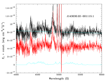
Figure 1: Unprocessed spectrum of SDSS J143030.22-001115.1 (left). Rest-frame spectra of SDSS J143030.22-001115.1 (right): the observed spectrum and a power-law continuum (top curve), Fe II-subtracted spectrum (middle curve), and Fe II spectrum (buttom curve).

3 RESULTS

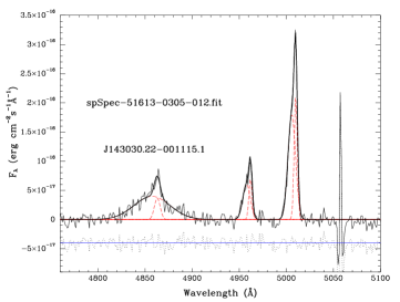
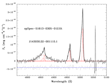
Figure 2: Multi-component fitting of the H$\beta$ and [O III]$\lambda\lambda$ 4959, 5007: modelled composite profile (thick solid line), individual components (the dotted lines), the residual spectrum (lower panel). Left: two components to model the H$\beta$ line; Right: three components to model the H$\beta$ line.

For SDSS J143030.22-001115.1, the [O III]$\lambda$5007 is very strong relative to $H\beta$ and the Fe II multiples are not too strong (See Fig. 1). The flux ratio of Fe II (between 4434 and 4684Å) to total H$\beta$ (Fe II$\lambda$ 4570/H$\beta$) is 0.59$\pm$ 0.17, which is much smaller than the mean value for the sample of 150 NLS1s (See Fig. 2 in Bian, Yuan & Zhao 2005).

In the left panel of Fig. 2, we showed two-component fitting of H$\beta$ and [O III]$\lambda\lambda$ 4959, 5007 for the rest-frame spectrum of SDSS J143030.22-001115.1. The FWHM, flux of each components are listed in Table 1.

Line	Component	Rest Wavelength	FWHM	Line flux
		($\AA$)	(km s-1)	($10^{-16}ergs^{-1}cm^{-2}$)
(1)	(2)	(3)	(4)	(5)
Two components to model the H$\beta$ line
H$\beta$	n	$4859.9\pm$ 1.1	$447\pm 199$	$2.8\pm 1.1$
	b	$4854.3\pm$ 1.1	$2785\pm 276$	$19.1\pm 1.2$
[O III]$\lambda$4959	n	$4960.6\pm$ 0.1	$238\pm 21$	$3.0\pm 0.5$
	b	$4956.5\pm$ 0.4	$563\pm 27$	$6.0\pm 0.5$
[O III]$\lambda$5007	n	$5006.8\pm$ 0.1	$238\pm 21$	$9.0\pm 1.5$
	b	$5002.60\pm$ 0.4	$563\pm 27$	$18.0\pm 1.5$
Three components to model the H$\beta$ line
H$\beta$	n1	$4862.6\pm$ 0.1	$231\pm 21$	$1.4\pm 0.3$
	n2	$4858.6\pm$ 0.4	$567\pm 25$	$1.9\pm 0.6$
	b	$4856.4\pm$ 1.2	$2911\pm 210$	$18.9\pm 1.1$
[O III]$\lambda$4959	n	$4960.6\pm$ 0.1	$231\pm 21$	$2.9\pm 0.4$
	b	$4956.5\pm$ 0.4	$567\pm 25$	$6.2\pm 0.5$
[O III]$\lambda$5007	n	$5006.8\pm$ 0.1	$231\pm 21$	$8.6\pm 1.2$
	b	$5002.6\pm$ 0.4	$567\pm 27$	$18.5\pm 1.5$
Starlight contribution and three components to model the H$\beta$ line
H$\beta$	n1	$4860.8\pm$ 0.5	$307\pm 44$	$2.4\pm 2.6$
	n2	$4855.4\pm$ 0.7	$408\pm 56$	$1.3\pm 2.7$
	b	$4856.7\pm$ 1.4	$2657\pm 154$	$15.7\pm 3.3$
[O III]$\lambda$4959	n	$4958.8\pm$ 0.5	$307\pm 44$	$5.6\pm 1.9$
	b	$4953.3\pm$ 0.7	$408\pm 56$	$4.3\pm 1.2$
[O III]$\lambda$5007	n	$5006.8\pm$ 0.5	$307\pm 44$	$16.8\pm 5.6$
	b	$5001.2\pm$ 0.7	$408\pm 56$	$12.9\pm 3.7$

Table 1: Results of the multi-component profile fitting of SDSS J143030.22-001115.1. Columns are: (1) emission line; (2) emission line components, where “n, n1, n2” and “b” represent the narrow and broad components, respectively; (3) the rest wavelength of the line component in angstroms; (4) FWHM of the line components (km s^-1); (5) integrated line flux ($10^{-16}ergs^{-1}cm^{-2}$).

From left panel of Fig. 2 and Table 1, we found that the line-intensity ratio of [O III]$\lambda$5007 to the narrow H$\beta$ is 9.6$\pm$ 3.8, which is consistent with the universal adopted value of 10 from the photoionization model for NLRs clouds. Considering the errors of the linewidth, the FWHM of the narrow H$\beta$ line is consistent with that of FWHM of the narrow and broad [O III] lines. The FWHM of the broad H$\beta$ line is 2785$\pm$ 276 km s^-1.

The template built from [O III] or [S II] is usually used to model narrow H$\beta$ and H$\alpha$ (Grupe et al. 1998; Grupe et al. 1999; Grupe et al. 2004; Greene & Ho, 2005a; 2005b). Since we used two-component profiles to model the asymmetric [O III]$\lambda$5007 profile, we should use three-component profiles to model H$\beta$, two components are coming from NLRs and one is BLRs. We take the same linewidth for each component of H$\beta$ and [O III] emitted from NLRs. And the flux ratio of [O III] to H$\beta$ from NLRs is set to be free. In the right panel of Fig. 2, we showed the three-component fitting of the H$\beta$ line. The FWHM, flux of each components are also listed in Table 2. The line-intensity ratio of [O III]$\lambda$5007 to the narrow H$\beta$ line is 8.2$\pm$ 3.2. The FWHM of the broad H$\beta$ line is 2911$\pm$ 210 km s^-1. Therefore, SDSS J143030.22-001115.1 is not a genuine NLS1 when we subtracted the H$\beta$ contribution from NLRs.

4 DISCUSSION

4.1 Black hole mass correction

NLS1s belong to seyfert 1 galaxies and were initially defined by their optical characteristics: FWHM(H$\beta$) less than 2000 km s^-1, which is usually used to calculate the central black hole virial mass (e.g. Wang & Lu 2001; Bian & Zhao 2004). We should use the line width of H$\beta$ coming from the BLRs to trace the BLRs virial movement. For SDSS J143030.22-001115.1, Williams et al. (2003) directly measured the width of the line halfway between the fitted continuum and the H$\beta$ line peak and obtained FWHM(H$\beta$) to be 1744 km s^-1. Considering the empirical size-luminosity formula and FWHM(H$\beta$) (Kaspi et al. 2000), we have calculate its central supermassive black hole mass using the value of 1744 km s^-1(Bian & Zhao 2004). Its mass is $10^{6.5}$  $\rm M_{\odot}$and its Eddington ratio log$L_{bol}/L_{Edd}$ is -0.60. Here we used the FWHM of broad H$\beta$ to recalculate the black hole mass. Its mass would be 0.44 larger if we take 2911 km s^-1as FWHM(H$\beta$), 0.41 larger if we take 2785 km s^-1as FWHM(H$\beta$). And log$L_{bol}/L_{Edd}$ would be -1.04$\sim$ -1.01. If we used the FWHM of narrow [O III] line to trace the bulge stellar velocity dispersion, we found SDSS J143030.22-001115.1 follow the so-called $M_{bh}-\sigma$ relation, $M_{\rm bh}=10^{8.13}(\frac{\sigma}{200{\rm km~{}s^{-1}}})^{4.02}\mbox{\,$\rm M_{\odot}$}$ (Tremaine et al. 2002).

For seven NLS1s, Rodriguez-Ardila et al. (2000) found that the narrow component of H$\beta$ (H$\beta_{n}$) is about, 50% of the total line flux and the [O III] $\lambda$5007/H$\beta_{n}$ ratio emitted in the NLRs varies from 1 to 5, instead of the universally adopted value of 10. We also found the [O III] is not too weak in many SDSS NLSls. This is consistent with the results of a sample of 64 NLSls presented by Veron-Cetty et al. (2001). When we calculate the virial black hole masses of NLS1s, we should measure the H$\beta$ linewidth after subtracting the H$\beta$ contribution from NLRs, which is especially important for NLS1s with luminous [O III] line. For the mass correction of other objects in the sample of 150 NLS1s and their locus in $M-\sigma$ plane, please referee to Bian, Yuan & Zhao (2006). There is no consideration about multi-component in $H\beta$ line in the traditional definition of NLS1s by Osterbrock & Pogge (1985) and Goodrich (1998). Therefor, we should cations about this traditional definition and just consider the H$\beta$ line from BLRs in this definition to classify NLS1s.

4.2 Starlight contribution

The fibers in SDSS have a diameter of 3” on the sky, corresponding to  6.5kpc at the redshift of SDSS J143030.22-001115.1. Its SDSS spectrum taken through such a fixed aperture includes most of the emission from the host galaxy emission (petroRad_r=3”.43). At the same time, the nuclear luminosity is comparable with its host galaxy (psfMag_r=18.85 and petroMag_r=17.9). Using the method of Lu et al. (2005) (Li et al. 2005; Hao et al. 2005), the stellar component is modelled. The results are showed in Fig. 3 and Table 3. The main conclusions are not changed.

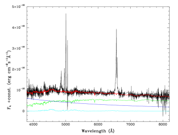
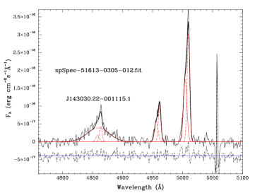
Figure 3: Left: the observed spectrum (black curve), a power-law continuum (middle blue curve), Fe II spectrum (bottom cyan curve), starlight contribution (middle Green curve), and composition of continuum, Fe II and starlight (red curve). Right: three components to model the H$\beta$ line.

4.3 X-ray photon index

ROSAT/ASCA X-ray observation of NLS1s showed that NLS1s generally have softer X-ray spectra than other AGNs, i.e. the larger photon index $\Gamma$, where $N_{E}\propto E^{-\Gamma}$ (e.g. Boller et al. 1996; Leighly 1999). Williams et al. (2004) suggested it is not always the case. They presented the Chandra observation of 17 NLS1s selected from the sample of 150 SDSS NLS1s (Williams et al. 2003). They derived $\Gamma$ from spectral fitting in Sherpa or hardness ratio. They found two objects have $\Gamma$ less than one: $0.25^{+0.80}_{-1.01}$ for SDSS J125943.59+010255.1, $0.92\pm 0.64$ for SDSS J143030.22-001115.1. For SDSS J125943.59+010255.1, its net Chandra 0.5-8keV count rate is $0.003\pm 0.001$ and the uncertainties of $\Gamma$ is too large. For SDSS J143030.22-001115.1, as we discussed above, it is not a genuine NLS1. We should remove these two objects to do the statistics of $\Gamma$ of NLS1s. The mean $\Gamma$ is $2.39\pm 0.15$ with the standard deviation of 0.59 when these two objects are excluded. Comparing with the result of Boller et al. (1996), the value of $\Gamma$ is smaller, which is partially due to the the different energy range coverage (Williams et al. 2004). It is suggested there is a correlation between $\Gamma$ and the accretion Eddington ratio (e.g. Bian & Zhao 2003; Grupe 2004; Williams et al. 2004; Bian 2005). There possibly exists NLS1s with smaller Eddington ratio and flat X-ray spectra.

It has been found that the optical properties of some NLS1s with flat X-ray spectrum are not quite different from those with steep X-ray spectrum. The Eddington ratio of the former may be smaller than the latter. NLS1s as presently defined are unlikely to be a homogeneous class. The apparent scarcity of ”NLS1s” with low Eddington ratio should result in selection effect: in flux limited surveys, it is difficult to find AGNs with small black hole and low mass accretion rate.

References

- [] Abazajian K., et al., 2005, AJ, 129,1755
- [] Bian W., Zhao, Y., 2003, MNRAS, 343, 164
- [] Bian W., Zhao, Y., 2004, MNRAS, 347, 607
- [] Bian W., 2005, ChJA&A, 5, S289
- [] Bian W., Yuan Q., Zhao Y., 2005, MNRAS, 364, 187
- [] Bian W., Yuan Q., Zhao Y., 2006, MNRAS, in press
- [] Boller Th., Brandt W. N., & Fink H. 1996, A&A, 305, 53
- [] Goodrich R.W., 1989, ApJ, 342, 224
- [] Boroson T. A., Green R. F., 1992, ApJS, 80, 109
- [] Greene J. E., Ho L. C., 2005a, ApJ, 627, 721
- [] Greene J. E., Ho L. C., 2005b, ApJ, 630, 122
- [] Greene J. E., Ho L. C., 2005c, ApJL, in press, astro-ph/0512461
- [] Grupe D., Wills B.J., Wills D., Beuermann K., 1998, A&A, 333, 827
- [] Grupe D., Beuermann K., Mannheim K., Thomas H.-C., 1999, A&A, 350, 805
- [] Grupe D., et al., 2004, AJ, 127, 156
- [] Grupe D., 2004, AJ, 127, 1799
- [] Gu Q. S., et al., 2005, MNRAS, in press, astro-ph/0510742
- [] Hao L., et al., 2005, AJ, 129, 1795
- [] Kaspi S., Smith P.S., Netzer H., Maoz D., Jannuzi B.T., Giveon U., 2000, ApJ, 533, 631
- [] Kriss G. A., 1994, in ASP Conf. Ser. 61, Astronomical Data Analysis Software and Systems III, ed. Crabtree D. R., Hanisch R. J., Barnes J. (San Francisco: ASP), 437
- [] Laor A., Fiore F., Elvis M., Wilkes B. J., McDowell J. C. 1997, ApJ, 477, 93
- [] Leighly K. M., 1999, ApJS, 125, 297
- [] Li C., et al., 2005, AJ, 129, 669
- [] Lu H., et al., 2005, AJ, in press, astro-ph/0510246
- [] Mineshige S., Kawaguchi T., Takeuchi M., Hayashida K., 2000, PASJ, 52, 499
- [] Osterbrock D.E., Pogge R., 1985, ApJ, 297, 166
- [] Pounds K. A., Done C., Osborne, 1995, MNRAS, 277, L5
- [] Rodriguez-Ardila A., et al., 2000, ApJ, 538, 581
- [] Stoughton C., et al., 2002, AJ, 123, 485
- [] Wandel A., Boller Th., 1998, A&A, 331, 884
- [] Wang T. G., Lu Y. J., 2001, A&A, 377, 52
- [] Williams R.J., Pogge R.W., Mathur S., 2003, AJ, 124, 3042
- [] Williams R. J., Mathur S., Pogge R. W., 2004, ApJ, 610, 737
- [] Tremaine S., et al., 2002, Ap J, 574, 740
- [] Veron-Cetty M.-P., Veron P., Goncalves A. C., 2001, A&A, 372, 730