Kinematic Dynamos using Constrained Transport
with High Order Godunov Schemes
and Adaptive Mesh Refinement

Abstract

We propose to extend the well-known MUSCL-Hancock scheme for Euler equations to the induction equation modeling the magnetic field evolution in kinematic dynamo problems. The scheme is based on an integral form of the underlying conservation law which, in our formulation, results in a “finite-surface” scheme for the induction equation. This naturally leads to the well-known “constrained transport” method, with additional continuity requirement on the magnetic field representation. The second ingredient in the MUSCL scheme is the predictor step that ensures second order accuracy both in space and time. We explore specific constraints that the mathematical properties of the induction equations place on this predictor step, showing that three possible variants can be considered. We show that the most aggressive formulations (referred to as C-MUSCL and U-MUSCL) reach the same level of accuracy as the other one (referred to as Runge-Kutta), at a lower computational cost. More interestingly, these two schemes are compatible with the Adaptive Mesh Refinement (AMR) framework. It has been implemented in the AMR code RAMSES. It offers a novel and efficient implementation of a second order scheme for the induction equation. We have tested it by solving two kinematic dynamo problems in the low diffusion limit. The construction of this scheme for the induction equation constitutes a step towards solving the full MHD set of equations using an extension of our current methodology.

1 Introduction

The extension of Godunov-type conservative schemes for Euler equations of fluid dynamics (Toro, 1999; Bouchut, 2005) to the system of ideal magnetohydrodynamics (MHD) has been a matter of intensive research, starting from the early 90’s. The great variety of different MHD implementations of the original Godunov method, especially in a multidimensional setting, has left several unexplored paths opened in designing MHD conservative methods.

The most natural approach in adapting finite-volume schemes to the MHD equations is to define the magnetic field component at the center of each cell, where the traditional hydrodynamical variables are also defined. One then takes advantage of decades of experience in the development of stable and accurate shock-capturing schemes. In this case, the solenoidality constraint $\mbox{\boldmath$\nabla$}\cdot\hbox{\bf B}=0$ has to be enforced using either a “divergence cleaning” step (see for example Brackbill and Barnes, 1980 and Ryu et al., 1998), or various reformulations of the MHD equations including additional divergence-waves (Powell et al., 1999) or divergence-damping terms (Dedner et al., 2002). A novel cell-centered MHD scheme has been recently developed by Crockett et al. (2005) that combines most of these ideas into one single algorithm.

An alternative approach is to use the Constrained Transport (CT) algorithm for the induction equation, as suggested in the late 60’s by Yee (1966), and later revisited by Evans and Hawley (1988). In this description, the magnetic field is defined at the cell faces, while other hydrodynamical variables are defined at the cell center. This is often called a “staggered mesh” discretization. As we will see in this paper, CT provides a natural expression of the induction equation in conservative form. Combining CT with the Godunov framework to design high-order, stable schemes is therefore a very attractive solution. This combined approach was first explored in the context of the MHD equations by Balsara and Spicer (1999). This method directly uses face-centered Godunov fluxes and averages these on the cell edges to estimate the Electro-Motive Force (EMF). Tóth (2000) proposed an interesting cell-centered alternative to this scheme. More recently, Londrillo and Del Zanna (2000, 2004) have revisited the problem and shown that the proper way of defining the edge-centered EMF is to solve a 2D Riemann problem at the cell edges. They have applied this idea to design high-order, Runge-Kutta, ENO schemes. Finally, Gardiner and Stone (2005) have extended Balsara and Spicer scheme to design a more stable and more robust way of computing the EMF.

The implementation of these various schemes within the Adaptive Mesh Refinement framework is another challenging issue. It introduces two main new technical difficulties: first, proper fluxes and EMF corrections between different levels of refinement must be accounted for. Second, when refining or de-refining cells, divergence-free preserving interpolation and prolongation operators must be designed. Both of these issues have recently been discussed in the framework of the CT algorithm by several authors (Balsara, 2001; Tóth and Roe, 2002; Li and Li, 2004).

The purpose of this article is to present a novel algorithm based on a high-order Godunov implementation of the CT algorithm within a tree-based Adaptive Mesh Refinement (AMR) code called RAMSES (Teyssier, 2002). As opposed to the grid-based (or patch-based) original AMR designed introduced by Berger and Oliger (1984) and Berger and Colella (1989), tree-based AMR trigger local grid refinements on a cell by cell basis. In this way, the grid follows more closely the geometrical features of the computed flow, at the cost of a greater algorithm’s complexity. Nevertheless, such tree-based AMR schemes have been implemented with success by various authors in the framework of astrophysics and fluid dynamics (Kravtsov et al., 1997; Khokhlov, 1998; Teyssier, 2002; Popinet, 2003) but not yet in the MHD context. On the other hand, patch-based AMR algorithms have been developed by several authors in recent years (Balsara, 2001; Kleimann et al., 2004; Powell et al., 1999; Samtaney et al., 2004; Ziegler, 1999) and used for MHD applications. The main requirement that tree-based AMR usually place on the underlying solver is the compactness of the computational stencil: any high order scheme with a stencil extending to two points, or less, in each direction can easily be coupled to an “octree” data structure (Khokhlov, 1998).

In this paper, our goal is to solve the induction equation using the MUSCL scheme, originally presented by van Leer (1977), and widely used in the literature for the Euler equations. This very simple method is second order accurate in time and space and has a compact stencil: only 2 neighboring cells in each direction (and for each dimension) are necessary to update the central cell solution to the next time step. This compactness property is of particular importance for our tree based AMR approach. It is also useful for an efficient parallelization relying on domain decomposition. To our knowledge, this is the first implementation of the MUSCL scheme combined with the Constrained Transport algorithm that solves the induction equation. The key ingredient that ensures second order accuracy is the so-called “predictor step”, in which the solution is first advanced by half a time step. We will consider a few different computational strategies for this predictor step and discuss their respective merits. Finally, we will present our overall tree-based AMR scheme.

This paper is limited to the induction equation. We intend to apply the same approach to the full MHD equations in a future paper. Nevertheless, it is interesting to determine if such a numerical approach can be applied to kinematic dynamo problems, for which the induction equation alone applies. The induction equation is linear, but it can yield remarkably rich magnetic instabilities corresponding to exponential field growth and referred to as “dynamo instabilities”. The description of these instabilities, and the conditions under which they occur, constitute an active field of research, with important consequences in astrophysics and in geophysics, since they account for the origin of magnetic fields in the Earth, planets, stars and even galaxies. We will restrict our attention here to well known dynamo flows and use them to investigate the numerical properties of our scheme.

An important problem in dynamo theory is related to a subclass of dynamo flows, known as “fast dynamos” which yield exponential field growth with finite growth rates in the limit of vanishing resistivity. This is of particular importance for astrophysical applications. Fast dynamos, when investigated with small, but finite, resistivity yield eigenmodes that are very localized in space, and are therefore ideal candidates for an investigation using the AMR scheme.

Dynamo problems have traditionally been studied using spectral methods (Galloway and Frisch, 1986; Christensen et al., 2001). Some recent models have been produced using finite differences (Archontis et al., 2003), finite volumes (Harder and Hansen, 2005) or finite elements (Matsui and Okuda, 2005). However, all of these methods rely on explicit physical diffusion to ensure numerical stability. The interest of using CT within the Godunov framework together with an AMR approach is twofold. First, fast dynamo modes have a very localized spatial structure (scaling as $Rm^{-1/2}$ where $Rm$ is the magnetic Reynolds number). Adapting the computational grid to the typical geometry of these modes therefore appears as a very natural strategy to minimize computational cost. Second, the Godunov methodology, using the CT scheme, introduces the minimal amount of numerical dissipation needed to ensure stability. This is an important property when using an AMR approach, for which cells of very different sizes coexist. This last property of the scheme is then mandatory to allow the use of a coarse grid in regions barely affected by the physical diffusion.

We will present several tests that demonstrate the efficiency of our tree-based AMR Godunov CT scheme for solving complex dynamo problems: we will first reproduce a simple advection problem of a magnetic loop and then validate the approach on two well known dynamo flows: the Ponomarenko dynamo and a fast ABC dynamo.

2 Constrained Transport in Two Space Dimensions

In this section, we briefly review the design of stable numerical schemes for hyperbolic systems of conservation laws in two space dimensions using the Godunov approach. Following Londrillo and Del Zanna (2000), such systems are called here “Euler systems”, as opposed to the “induction system” we will consider later.

2.1 First Order Godunov Scheme for Euler systems

We first examine the problem in one space dimension. The following Euler system,

$$\frac{\partial\hbox{\bf U}}{\partial t}+\mbox{\boldmath$\nabla$}\cdot\hbox{\bf F}(\hbox{\bf U})=0\,,$$ (1)

can be written in integral form by defining finite control volume elements in space and time, where we define a cell by $V_{i}=[x_{i-{\textstyle\frac{1}{2}}},x_{i+{\textstyle\frac{1}{2}}}]$ and a time interval by $\Delta t=t^{n+1}-t^{n}$. The conservative system writes for each cell $V_{i}$

$$\left<U\right>_{i}^{n+1}-\left<U\right>_{i}^{n}+\frac{\Delta t}{\Delta x}\left(F_{i+{\textstyle\frac{1}{2}}}^{n+{\textstyle\frac{1}{2}}}-F_{i-{\textstyle\frac{1}{2}}}^{n+{\textstyle\frac{1}{2}}}\right)=0\,.$$ (2)

Note that this integral form is exact for the corresponding Euler system. The averaged, cell-centered state is defined by

$$\left<U\right>_{i}^{n}=\frac{1}{\Delta x}\int_{x_{i-{\textstyle\frac{1}{2}}}}^{x_{i+{\textstyle\frac{1}{2}}}}U(x,t^{n})\,{\rm d}x\,,$$ (3)

while the averaged, time-centered intercell flux is defined by

$$F_{i+{\textstyle\frac{1}{2}}}^{n+{\textstyle\frac{1}{2}}}=\frac{1}{\Delta t}\int_{t^{n}}^{t_{n+1}}F(x_{i+{\textstyle\frac{1}{2}}},t)\,{\rm d}t\,.$$ (4)

The Godunov method states that the intercell flux is computed using the solution of a Riemann problem with left and right states given by the left and right averaged states

$$U^{*}_{i+{\textstyle\frac{1}{2}}}(x/t)=RP\left[\left<U\right>_{i}^{n},\left<U\right>_{i+1}^{n}\right]\,.$$ (5)

This approach, called “first order Godunov scheme”, assumes that the solution inside cell $V_{i}$ is piecewise constant. Taking advantage of the self-similarity of the Riemann solution for initially piecewise constant states, one can simplify further the time-average of the flux and obtain

$$F_{i+{\textstyle\frac{1}{2}}}^{n+{\textstyle\frac{1}{2}}}=F(U^{*}_{i+{\textstyle\frac{1}{2}}}(0))\,.$$ (6)

Note that again the time evolution of the average state over one time step is exact. Numerical approximations arise when one assumes at the next time step that the new solution inside cell $V_{i}$ is also piecewise constant and equal to the new averaged state.

We now extend the previous method to Euler systems in 2 space dimensions. The conservative system can also be written in the following unsplit formulation

$$\left<U\right>_{i,j}^{n+1}-\left<U\right>_{i,j}^{n}+\frac{\Delta t}{\Delta x}\left(F_{i+{\textstyle\frac{1}{2}},j}^{n+{\textstyle\frac{1}{2}}}-F_{i-{\textstyle\frac{1}{2}},j}^{n+{\textstyle\frac{1}{2}}}\right)+\frac{\Delta t}{\Delta y}\left(G_{i,j+{\textstyle\frac{1}{2}}}^{n+{\textstyle\frac{1}{2}}}-G_{i,j-{\textstyle\frac{1}{2}}}^{n+{\textstyle\frac{1}{2}}}\right)=0\,,$$ (7)

where the average state is now defined over a 2 dimensional cell $V_{i,j}$, and intercell fluxes are now time averaged fluxes integrated over the line separating neighboring cells

$$F_{i+{\textstyle\frac{1}{2}},j}^{n+{\textstyle\frac{1}{2}}}=\frac{1}{\Delta t}\frac{1}{\Delta y}\int_{t^{n}}^{t_{n+1}}\int_{y_{j-{\textstyle\frac{1}{2}}}}^{y_{j+{\textstyle\frac{1}{2}}}}F(x_{i+{\textstyle\frac{1}{2}}},y,t)\,{\rm d}t\,{\rm d}y\,,$$ (8)

$$G_{i,j+{\textstyle\frac{1}{2}}}^{n+{\textstyle\frac{1}{2}}}=\frac{1}{\Delta t}\frac{1}{\Delta x}\int_{t^{n}}^{t_{n+1}}\int_{x_{i-{\textstyle\frac{1}{2}}}}^{x_{i+{\textstyle\frac{1}{2}}}}G(x,y_{j+{\textstyle\frac{1}{2}}},t)\,{\rm d}t\,{\rm d}x\,.$$ (9)

At this point, the integral form is still exact. The generalization of the 1D Godunov scheme to multidimensional problems now relies on solving two dimensional Riemann problems at each corner, defined by four initially piecewise constant states

$$U^{*}_{i+{\textstyle\frac{1}{2}},j+{\textstyle\frac{1}{2}}}(x/t,y/t)=RP\left[\left<U\right>_{i,j}^{n},\left<U\right>_{i+1,j}^{n}\left<U\right>_{i,j+1}^{n}\left<U\right>_{i+1,j+1}^{n}\right]\,.$$ (10)

The fundamental difference with the 1D case is that we now need to average the complete solutions of 2 adjacent Riemann solutions over the entire transverse line segment, where fluxes are defined. These space-averaged fluxes are not functions of a unique self-similar variable anymore, but depend explicitly on time. Building such a numerical scheme is barely possible for simple scalar linear advection problem and far too complex to implement for non-linear systems.

The traditional approach is to approximate the true solution using a predictor-corrector scheme. This is also the key ingredient of any high-order scheme, where the self-similarity of the Riemann problem breaks down, even in one space dimension, due to the underlying piecewise linear or parabolic representation of the data. The idea is to compute a predicted state at time level $t^{n+1/2}$ and to use this intermediate state as an input state for the two final 1D Riemann solvers.

We list here 3 classical methods to implement this predictor step

• Godunov method: no predictor step is performed. This greatly simplifies the method, which now relies on one Riemann solver in each direction. The prize to pay is a somewhat restrictive Courant stability condition: $(u/\Delta x+v/\Delta y)\Delta t\leq 1$, where $u$ and $v$ are the maximum wave speed in each direction.

• Runge-Kutta method: the predictor step is performed using the 2D Godunov method with half the time step. The resulting intermediate states are then used to compute the fluxes for the final conservative update. The Courant condition is the same as for the Godunov method, but one has to perform 2 Riemann solvers per cell in each direction (4 in total).

• Corner Transport Upwind method: predicted states for a given Riemann problem are computed with a 1D update in the transverse direction only, for the time interval $\Delta t/2$. This scheme was first proposed by Colella (1990). It allows up to a factor of two larger time steps than the two previous schemes, since the Courant condition is now $\max(u/\Delta x,v/\Delta y)\Delta t\leq 1$, but 2 Riemann solvers per cell in each direction (4 in total) are still needed.

All three methods are directionally unsplit, first order approximations (in space) of the underlying Euler system.

2.2 First Order Godunov Scheme for the Induction Equation

The magnetic field evolution in the MHD approximation is governed by the induction equation which neglects free charge density and displacement currents. It is written in conservative form as

$$\frac{\partial\hbox{\bf B}}{\partial t}=\mbox{\boldmath$\nabla$}\times\hbox{\bf E}+\eta\,\Delta\hbox{\bf B}\,,$$ (11)

where the EMF E is given by

$$\hbox{\bf E}=\hbox{\bf v}\times\hbox{\bf B}\,,$$ (12)

and $\eta$ is the magnetic diffusivity. The magnetic field also satisfies the divergence free constraint

$$\mbox{\boldmath$\nabla$}\cdot\hbox{\bf B}=0\,.$$ (13)

It is usually more convenient to consider (11) in non-dimensional form by introducing a typical lengthscale ${\mathcal{L}}$ and a typical timescale ${\mathcal{T}}={\mathcal{L}}/U$ where $U$ is some norm of the velocity (usually based on the maximal value over space and time). The resulting non-dimensional equation is

$$\frac{\partial\hbox{\bf B}}{\partial\tilde{t}}=\mbox{\boldmath$\nabla$}\times\left(\tilde{\hbox{\bf v}}\times\hbox{\bf B}\right)+\mbox{Rm}^{-1}\,\,\Delta\hbox{\bf B}\,,$$ (14)

where $\mbox{Rm}=(U{\mathcal{L}})/\eta$ while $\tilde{t}=t/{\mathcal{T}}$ and $\tilde{\hbox{\bf v}}=\hbox{\bf v}/U$ are respectively the non-dimensionnal time and velocities and the spatial derivative are taken with respect to normalized distances.

The EMF E is here the analog of the flux function for Euler systems. We now restrict our attention to 2D dimensional flows, for which only one component of the EMF, say $E_{z}$, is sufficient.

Following the Godunov approach, we write the 2D induction equation in integral form over a finite control volume in space and time. For the $B_{x}$ component of the magnetic field, we define a finite surface element $S_{i+1/2,j}=[y_{j-1/2},y_{j+1/2}]$ at position $x_{i+1/2}$

$$\left<B_{x}\right>_{i+{\textstyle\frac{1}{2}},j}^{n+1}=\left<B_{x}\right>_{i+{\textstyle\frac{1}{2}},j}^{n}+\frac{\Delta t}{\Delta y}\left(\left<E_{z}\right>_{i+{\textstyle\frac{1}{2}},j+{\textstyle\frac{1}{2}}}^{n+{\textstyle\frac{1}{2}}}-\left<E_{z}\right>_{i+{\textstyle\frac{1}{2}},j-{\textstyle\frac{1}{2}}}^{n+{\textstyle\frac{1}{2}}}\right)\,.$$ (15)

For the $B_{y}$ component, we define a finite surface element $S_{i,j+1/2}=[x_{i-1/2},x_{j+1/2}]$ at position $y_{i+1/2}$. The induction equation in integral form has a similar representation

$$\left<B_{y}\right>_{i,j+{\textstyle\frac{1}{2}}}^{n+1}=\left<B_{y}\right>_{i,j+{\textstyle\frac{1}{2}}}^{n}-\frac{\Delta t}{\Delta x}\left(\left<E_{z}\right>_{i+{\textstyle\frac{1}{2}},j+{\textstyle\frac{1}{2}}}^{n+{\textstyle\frac{1}{2}}}-\left<E_{z}\right>_{i-{\textstyle\frac{1}{2}},j+{\textstyle\frac{1}{2}}}^{n+{\textstyle\frac{1}{2}}}\right)\,.$$ (16)

Note that this integral form in space and time is exact. The average, surface centered, magnetic states are defined as the average magnetic field components on their corresponding control surfaces

$$\left<B_{x}\right>_{i+{\textstyle\frac{1}{2}},j}^{n}=\frac{1}{\Delta y}\int_{y_{i-{\textstyle\frac{1}{2}}}}^{y_{i+{\textstyle\frac{1}{2}}}}B_{x}(x_{i+{\textstyle\frac{1}{2}}},y,t^{n})\,{\rm d}y\,,$$ (17)

$$\left<B_{y}\right>_{i,j+{\textstyle\frac{1}{2}}}^{n}=\frac{1}{\Delta x}\int_{x_{i-{\textstyle\frac{1}{2}}}}^{x_{i+{\textstyle\frac{1}{2}}}}B_{y}(x,y_{i+{\textstyle\frac{1}{2}}},t^{n})\,{\rm d}x\,.$$ (18)

2.2.1 2D Riemann Problem

The time centered EMF results from a time average at the corner points

$$\left<E_{z}\right>_{i+{\textstyle\frac{1}{2}},j+{\textstyle\frac{1}{2}}}^{n+{\textstyle\frac{1}{2}}}=\frac{1}{\Delta t}\int_{t^{n}}^{t_{n+1}}E_{z}(x_{i+{\textstyle\frac{1}{2}}},y_{j+{\textstyle\frac{1}{2}}},t)\,{\rm d}t\,.$$ (19)

Let us now apply the Godunov method to the 2D induction equation. Upon noticing that our initial conditions are given by four piecewise constant states around each corner points, we can use the self-similar solution of the 2D Riemann problem at the corner point,

$$U^{*}_{i+{\textstyle\frac{1}{2}},j+{\textstyle\frac{1}{2}}}(x/t,y/t)=RP\left[\left<U\right>_{i,j}^{n},\left<U\right>_{i+1,j}^{n}\left<U\right>_{i,j+1}^{n}\left<U\right>_{i+1,j+1}^{n}\right]\,,$$ (20)

and time integration vanishes in equation (19)

$$\left<E_{z}\right>_{i+{\textstyle\frac{1}{2}},j+{\textstyle\frac{1}{2}}}^{n+{\textstyle\frac{1}{2}}}=E_{z}(U^{*}_{i+{\textstyle\frac{1}{2}},j+{\textstyle\frac{1}{2}}}(0,0))\,.$$ (21)

The Godunov method, applied to the induction equation in 2D, shares this interesting property with the Godunov method applied to 1D Euler system. The self-similarity of the flux function was lost for 2D Euler systems. The self-similarity of the EMF function is still valid for the 2D induction equation, provided our initial conditions are described by piecewise constant states. We will see in the next section, that this is unfortunately not true in the general case, even at lowest order.

\psfrag{ijk}{\small$(i,j,k)$}\psfrag{ijpk}{\small$(i,j\!+\!1,k)$}\psfrag{ipjpk}{\small\ \ \ $(i\!+\!1,j\!+\!1,k)$}\psfrag{ipjk}{\small\ $(i\!+\!1,j,k)$}\psfrag{x}{\footnotesize{\bf x}}\psfrag{y}{\footnotesize{\bf y}}\includegraphics[width=170.71652pt]{scheme2D.eps}

Figure 1: The 2D Riemann problem in the x-y plane to compute the EMF in the z direction at edge ($i+{\textstyle\frac{1}{2}}$, $j+{\textstyle\frac{1}{2}}$). The face-centered magnetic fields are shown as vertical and horizontal arrows. The velocity field is shown as the dashed arrow.

As noticed by Londrillo and Del Zanna (2000), the 2D Riemann problem is the key ingredient for solving the induction equation with a stable (upwind) scheme. The 4 initial states (with 2 magnetic field components per state) need to satisfy the $\mbox{\boldmath$\nabla$}\cdot\hbox{\bf B}=0$ property. $B_{x}$ should therefore be the same for the two top states, and for the two bottom states, while $B_{y}$ should be the same for the two left states, and for the two right states (see Fig. 1). This condition is naturally satisfied as long as magnetic field is defined as a surface-average, see (17) and (18).

In the general MHD case, designing 2D Riemann solvers (even approximate ones) is a very ambitious task. For the kinematic induction case, the solution is however remarkably simple, since the solution is nothing else but the upwind state. The edge-centered EMF can therefore be written in the following closed form

$$\left<E_{z}\right>_{i+{\textstyle\frac{1}{2}},j+{\textstyle\frac{1}{2}}}^{n+{\textstyle\frac{1}{2}}}=u\frac{\left<B_{y}\right>_{i+1,j+{\textstyle\frac{1}{2}}}+\left<B_{y}\right>_{i,j+{\textstyle\frac{1}{2}}}}{2}-v\frac{\left<B_{x}\right>_{i+{\textstyle\frac{1}{2}},j+1}+\left<B_{x}\right>_{i+{\textstyle\frac{1}{2}},j}}{2}$$

$$-\left|u\right|\frac{\left<B_{y}\right>_{i+1,j+{\textstyle\frac{1}{2}}}-\left<B_{y}\right>_{i,j+{\textstyle\frac{1}{2}}}}{2}+\left|v\right|\frac{\left<B_{x}\right>_{i+{\textstyle\frac{1}{2}},j+1}-\left<B_{x}\right>_{i+{\textstyle\frac{1}{2}},j}}{2}\,,$$ (22)

where $u$ and $v$ are respectively the $x$ and $y$ components of the flow velocity $\hbox{\bf v}=(u,v,w)$ computed at the center of the edge $(i+{\textstyle\frac{1}{2}},j+{\textstyle\frac{1}{2}})$. This last equation is familiar in the framework of upwind finite-volume schemes. It can be decomposed into two contributions. The first line is the EMF computed using the average magnetic fields at the cell corners: this EMF is a second-order in space. The resulting scheme (retaining this term only) would have been unconditionally unstable, if it was not for the second term, the contribution of the upwinding. It is equivalent to a 2D numerical diffusivity, with directional diffusivity coefficients given by $\eta_{x}=\left|u\right|\Delta x/2$ and $\eta_{y}=\left|v\right|\Delta y/2$. This (relatively large) resistivity introduces the minimal but necessary amount of numerical diffusion for the scheme to remain stable.

2.2.2 Constrained Transport as a Finite Surface Approximation

This straightforward extension of the Godunov methodology has lead us to the well known “Constrained Transport” (CT) scheme, that was designed a long time ago for the MHD equations by Yee (1966). The key property of the CT scheme is that one can also write the $\mbox{\boldmath$\nabla$}\cdot\hbox{\bf B}=0$ constraint in integral form as

$$\frac{\left<B_{x}\right>_{i+{\textstyle\frac{1}{2}},j}^{n}-\left<B_{x}\right>_{i-{\textstyle\frac{1}{2}},j}^{n}}{\Delta x}+\frac{\left<B_{y}\right>_{i,j+{\textstyle\frac{1}{2}}}^{n}-\left<B_{y}\right>_{i,j-{\textstyle\frac{1}{2}}}^{n}}{\Delta y}=0\,.$$ (23)

This integral form is exact. Moreover, if it is satisfied by our initial data, the integral forms in (15) and (16) ensure that it will be satisfied at all iterations during the numerical integration. Using equation (23), and assuming that formally $\Delta x\rightarrow 0$, we show that the following property holds:

Remark 1

$\left<B_{x}\right>_{j}^{n}(x)$ is a continuous function of coordinate $x$,

and, symmetrically, assuming that formally $\Delta y\rightarrow 0$, we have:

Remark 2

$\left<B_{y}\right>_{i}^{n}(y)$ is a continuous function of coordinate $y$,

This means that $\left<B_{x}\right>_{i+1/2,j}^{n}$ can be considered as piecewise constant in the y direction, but has to be considered as piecewise linear in the x direction. This constitutes our lowest order approximation of the magnetic field. Symmetrically, to lowest order, $\left<B_{y}\right>_{i,j+1/2}^{n}$ can be considered as piecewise constant in the x direction, but has to be considered as piecewise linear in the y direction.

This last property provides a fundamental difference between the induction equations and Euler systems. It is due to the divergence free constraint, expressed in integral form on a staggered magnetic field representation. One consequence of this property is that our initial state for the 2D Riemann problem cannot be piecewise constant anymore, but instead piecewise linear. We therefore loose the property of self-similarity for the Riemann solution at corner points, and cannot perform an exact time integration to compute the time average EMF. We now have to rely on approximations. Following the strategies developed in section 2.1, we approximate the time averaged EMF using various predictor-corrector schemes.

2.3 The Predictor step

2.3.1 Godunov Scheme

The first possibility is to drop the predictor step and solve the Riemann problem defined at time $t^{n}$. Using (15) and (16), together with the EMF computed from (22), we obtain the Godunov scheme for the induction equation. In the simple case of a constant velocity field with $u>0$ and $v>0$ (the pure advection case), we can write the overall scheme as

$$\left<B_{x}\right>_{i+{\textstyle\frac{1}{2}},j}^{n+1}=\left<B_{x}\right>_{i+{\textstyle\frac{1}{2}},j}^{n} + u\frac{\Delta t}{\Delta y}\left(\left<B_{y}\right>_{i,j+{\textstyle\frac{1}{2}}}^{n}-\left<B_{y}\right>_{i,j-{\textstyle\frac{1}{2}}}^{n}\right)$$ (24)

$$- v\frac{\Delta t}{\Delta y}\left(\left<B_{x}\right>_{i+{\textstyle\frac{1}{2}},j}^{n}-\left<B_{x}\right>_{i+{\textstyle\frac{1}{2}},j-1}^{n}\right)\,.$$

Using the $\mbox{\boldmath$\nabla$}\cdot\hbox{\bf B}=0$ constraint at time $t^{n}$ in integral form (23), we further simplify the scheme to obtain

$$\left<B_{x}\right>_{i+{\textstyle\frac{1}{2}},j}^{n+1}=\left<B_{x}\right>_{i+{\textstyle\frac{1}{2}},j}^{n} - u\frac{\Delta t}{\Delta x}\left(\left<B_{x}\right>_{i+{\textstyle\frac{1}{2}},j}^{n}-\left<B_{x}\right>_{i-{\textstyle\frac{1}{2}},j}^{n}\right)$$ (25)

$$- v\frac{\Delta t}{\Delta y}\left(\left<B_{x}\right>_{i+{\textstyle\frac{1}{2}},j}^{n}-\left<B_{x}\right>_{i+{\textstyle\frac{1}{2}},j-1}^{n}\right)\,.$$

We can therefore conclude:

Proposition 1

For the advection case, if the initial data satisfy the integral form of the solenoidality constraint, the Godunov method for the induction equation is identical to the Godunov method for the advection equation on the staggered grid.

This rather simple point is actually quite important, since it proves that CT has advection properties quite similar (in this case identical) to traditional finite-volume methods. The Godunov scheme for the induction equation has a compact stencil. It is however of mere theoretical interest, since, as we will see in the next section, it is not the first order limit of higher order Godunov implementations of the induction equation.

Runge-Kutta                         U-MUSCL                         C-MUSCL

       

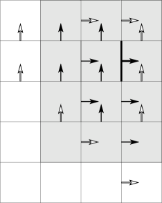
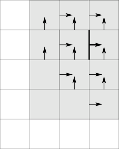
Figure 2: Stencils of our various schemes for the induction equation: Runge-Kutta scheme (left plot), U-MUSCL scheme (middle plot) and C-MUSCL scheme (right plot). The flux being computed is indicated by a bold face and arrow. For the purpose of this example, the velocity field is pointing in the upper right direction ($u>0$ and $v>0$). The first order stencil in space (second order in time) is represented with black arrows. Additional components required for the second order stencils in time and space are shown with white arrows. The shaded region indicates cells that are available in a tree-based AMR implementation. Only the two right schemes have stencils compact enough for such an implementation.

2.3.2 Runge-Kutta Scheme

As discussed above, the $\mbox{\boldmath$\nabla$}\cdot\hbox{\bf B}=0$ constraint, and the loss of self-similarity in the Riemann solution, pushes towards using a predictor step in designing our first order scheme. The most natural approach is the Runge-Kutta scheme, for which the solution is advanced first to the intermediate time coordinate $t^{n+1/2}$, using the (previously described) Godunov scheme with time step $\Delta t/2$. These predicted states are then used to define the 4 initial states for the 2D Riemann problem. The resulting EMF is used to advance the solution from time $t^{n}$ to the next time coordinate $t^{n+1}$ with time step $\Delta t$. A similar, 2 step, Runge-Kutta method for the induction equation is used for example in Londrillo and Del Zanna (2000) and Londrillo and Del Zanna (2004) to solve the MHD equations.

Using similar arguments as in the previous section, it is easy to show that, for a uniform velocity field, since the predicted magnetic field satisfies the integral form of the solenoidality constraint, the corrector step for the induction equation is identical to the predictor step for the advection equation. As we have shown in the last section, this property also holds for the predictor step, we therefore obtain a second important result:

Proposition 2

For a uniform velocity field, if the initial data satisfy the integral form of the solenoidality constraint, the Runge-Kutta method for the induction equation is identical to the Runge-Kutta method for the advection equation on the staggered grid.

We will show later that it is also possible to design higher order schemes for this algorithm. This scheme has two nice properties: it is second order in time (while still first order in space), and the predicted magnetic field satisfies exactly $\mbox{\boldmath$\nabla$}\cdot\hbox{\bf B}^{n+1/2}=0$. There are also issues associated with it, especially in the AMR framework. It can be easily shown (see Fig. 2) that the stencil is not compact enough for a tree-based AMR: 3 ghost cells are needed in each direction (resp. 2) for the second order (resp. first order) scheme. We will see in the test section that it is also slightly more diffusive than the other schemes we will describe in the following sections. The Courant stability condition is also rather restrictive

$$\left(\frac{u}{\Delta x}+\frac{v}{\Delta y}\right)\Delta t\leq 1\,.$$ (26)

2.3.3 Upwind-MUSCL Scheme

When deriving the MUSCL scheme for Euler systems, van Leer (1977) noticed that it was not necessary for the predictor step to be strictly conservative. A conservative update was however mandatory for the corrector step. Similarly, for the induction equation, it is a priori not necessary for the predictor step to satisfy the solenoidality constraint. It is however mandatory for the initial and final data. Instead of computing one EMF at each cell corner, using a 2D Riemann solver, we now propose to compute for the predictor step only 4 EMFs at each cell corner, corresponding to each input magnetic field.

These EMFs are defined as $\left<E_{z}\right>_{i+1/2,j+1/2}^{L}$, $\left<E_{z}\right>_{i+1/2,j+1/2}^{R}$, $\left<E_{z}\right>_{i+1/2,j+1/2}^{B}$ and $\left<E_{z}\right>_{i+1/2,j+1/2}^{T}$, where each upper index corresponds to the “left”, “right”, “bottom” and “top” face, respectively. Each EMF is specialized to its corresponding face-centered magnetic field component. One EMF per face is allowed, in order to satisfy the continuity constraint: we need to solve a 1D Riemann problem in the perpendicular direction. The Riemann solution is here the “upwind” state. The “bottom” and “top” EMF for the predictor step are therefore

$$\left<E_{z}\right>_{i+{\textstyle\frac{1}{2}},j+{\textstyle\frac{1}{2}}}^{B} = u\left({\left<B_{y}\right>_{i+1,j+{\textstyle\frac{1}{2}}}+\left<B_{y}\right>_{i,j+{\textstyle\frac{1}{2}}}}\right)/{2}-v\left<B_{x}\right>_{i+{\textstyle\frac{1}{2}},j}$$

$$- \left|u\right|\left({\left<B_{y}\right>_{i+1,j+{\textstyle\frac{1}{2}}}-\left<B_{y}\right>_{i,j+{\textstyle\frac{1}{2}}}}\right)/{2}\,,$$

$$\left<E_{z}\right>_{i+{\textstyle\frac{1}{2}},j+{\textstyle\frac{1}{2}}}^{T} = u\left({\left<B_{y}\right>_{i+1,j+{\textstyle\frac{1}{2}}}+\left<B_{y}\right>_{i,j+{\textstyle\frac{1}{2}}}}\right)/{2}-v\left<B_{x}\right>_{i+{\textstyle\frac{1}{2}},j+1}$$ (27)

$$- \left|u\right|\left({\left<B_{y}\right>_{i+1,j+{\textstyle\frac{1}{2}}}-\left<B_{y}\right>_{i,j+{\textstyle\frac{1}{2}}}}\right)/{2}\,.$$

Similarly, the “left” and “right” EMF are

$$\left<E_{z}\right>_{i+{\textstyle\frac{1}{2}},j+{\textstyle\frac{1}{2}}}^{L}=u\left<B_{y}\right>_{i,j+{\textstyle\frac{1}{2}}} - v\left({\left<B_{x}\right>_{i+{\textstyle\frac{1}{2}},j+1}+\left<B_{x}\right>_{i+{\textstyle\frac{1}{2}},j}}\right)/{2}$$

$$+ \left|v\right|\left({\left<B_{x}\right>_{i+{\textstyle\frac{1}{2}},j+1}-\left<B_{x}\right>_{i+{\textstyle\frac{1}{2}},j}}\right)/{2}\,,$$

$$\left<E_{z}\right>_{i+{\textstyle\frac{1}{2}},j+{\textstyle\frac{1}{2}}}^{R}=u\left<B_{y}\right>_{i+1,j+{\textstyle\frac{1}{2}}} - v\left({\left<B_{x}\right>_{i+{\textstyle\frac{1}{2}},j+1}+\left<B_{x}\right>_{i+{\textstyle\frac{1}{2}},j}}\right)/{2}$$ (28)

$$+ \left|v\right|\left({\left<B_{x}\right>_{i+{\textstyle\frac{1}{2}},j+1}-\left<B_{x}\right>_{i+{\textstyle\frac{1}{2}},j}}\right)/{2}\,.$$

The predictor step for the x component of the magnetic field becomes

$$\left<B_{x}\right>_{i+{\textstyle\frac{1}{2}},j}^{n+1/2}=\left<B_{x}\right>_{i+{\textstyle\frac{1}{2}},j}^{n}+\frac{\Delta t}{2\Delta y}\left(\left<E_{z}\right>_{i+{\textstyle\frac{1}{2}},j+{\textstyle\frac{1}{2}}}^{B}-\left<E_{z}\right>_{i+{\textstyle\frac{1}{2}},j-{\textstyle\frac{1}{2}}}^{T}\right)\,,$$ (29)

and for the y component we have

$$\left<B_{y}\right>_{i,j+{\textstyle\frac{1}{2}}}^{n+1/2}=\left<B_{y}\right>_{i,j+{\textstyle\frac{1}{2}}}^{n}-\frac{\Delta t}{2\Delta x}\left(\left<E_{z}\right>_{i+{\textstyle\frac{1}{2}},j+{\textstyle\frac{1}{2}}}^{L}-\left<E_{z}\right>_{i-{\textstyle\frac{1}{2}},j+{\textstyle\frac{1}{2}}}^{R}\right)\,.$$ (30)

To complete this scheme, the corrector step is performed using a final 2D Riemann solver to compute the time-centered EMF (22) and a final conservative update of each magnetic field component (15) and (16).

Let us now examine the property of the Upwind–MUSCL scheme in the case of a uniform velocity field. We can assume, without loss of generality, that $u>0$ and $v>0$. In this case, the predicted state can be written in a more compact form

$$\left<B_{x}\right>_{i+{\textstyle\frac{1}{2}},j}^{n+1/2}=\left<B_{x}\right>_{i+{\textstyle\frac{1}{2}},j}^{n}+u\frac{\Delta t}{2\Delta y}\left(\left<B_{y}\right>_{i,j+{\textstyle\frac{1}{2}}}^{n}-\left<B_{y}\right>_{i,j-{\textstyle\frac{1}{2}}}^{n}\right)\,,$$ (31)

which is equivalent, using (23), to

$$\left<B_{x}\right>_{i+{\textstyle\frac{1}{2}},j}^{n+1/2}=\left<B_{x}\right>_{i+{\textstyle\frac{1}{2}},j}^{n}-u\frac{\Delta t}{2\Delta x}\left(\left<B_{x}\right>_{i+{\textstyle\frac{1}{2}},j}^{n}-\left<B_{x}\right>_{i-{\textstyle\frac{1}{2}},j}^{n}\right)\,.$$ (32)

Similar expressions can be derived for $\left<B_{y}\right>_{i,j+1/2}^{n+1/2}$. Inserting these predicted values into (22) and (15), we get, after some tedious manipulations, the final updated solution

$$\left<B_{x}\right>_{i+{\textstyle\frac{1}{2}},j}^{n+1} = \left<B_{x}\right>_{i+{\textstyle\frac{1}{2}},j}^{n}\left(1-C_{x}\right)\left(1-C_{y}\right)+\left<B_{x}\right>_{i-{\textstyle\frac{1}{2}},j}^{n}C_{x}\left(1-C_{y}\right)$$ (33)

$$+ \left<B_{x}\right>_{i+{\textstyle\frac{1}{2}},j-1}^{n}C_{y}\left(1-C_{x}\right)+\left<B_{x}\right>_{i-{\textstyle\frac{1}{2}},j-1}^{n}C_{x}C_{y}\,,$$

where the following definitions have been used $C_{x}=u\Delta t/\Delta x$ and $C_{y}=v\Delta t/\Delta y$. One can recognize here the Corner Transport Upwind (CTU) advection scheme presented in Colella (1990), for which the Courant stability condition is

$$\max\left[\frac{u}{\Delta x},\frac{v}{\Delta y}\right]\Delta t\leq 1\,.$$ (34)

We therefore conclude:

Proposition 3

For a uniform velocity field, if the initial data satisfy the integral form of the solenoidality constraint, the Upwind-MUSCL Scheme for the induction equation is identical to Colella’s first order CTU scheme for the advection equation on the staggered grid.

It is apparent in (33) that the stencil of this MUSCL scheme is more compact that it is for the Runge-Kutta scheme (see also Fig. 2). Since our goal is here to develop an AMR code for the induction equation, this is a very attractive solution. The predictor step is performed using upwinding in the normal direction. As for Colella’s CTU scheme, the Courant stability condition is very efficient. We now explore one last possibility for our MUSCL predictor step.

2.3.4 Conservative-MUSCL Scheme

The last scheme was designed in dropping the solenoidality constraint for the predictor step. We propose in this section to drop the upwinding in the EMF computation for the predictor step, which now becomes

$$\left<E_{z}\right>_{i+{\textstyle\frac{1}{2}},j+{\textstyle\frac{1}{2}}}^{n}=u\frac{\left<B_{y}\right>_{i+1,j+{\textstyle\frac{1}{2}}}^{n}+\left<B_{y}\right>_{i,j+{\textstyle\frac{1}{2}}}^{n}}{2}-v\frac{\left<B_{x}\right>_{i+{\textstyle\frac{1}{2}},j+1}^{n}+\left<B_{x}\right>_{i+{\textstyle\frac{1}{2}},j}^{n}}{2}\,.$$

Since we now have a single EMF per cell corner, the predicted magnetic field satisfies by construction $\mbox{\boldmath$\nabla$}\cdot\hbox{\bf B}^{n+1/2}=0$. The corrector step is the same as for all 3 methods. Here again, we would like to examine the property of the scheme for the case of uniform advection. Because in this case $\mbox{\boldmath$\nabla$}\cdot\hbox{\bf B}^{n+1/2}=0$, the corrector step is identical to the corrector step for the Godunov advection scheme on the staggered grid. The predictor step, on the other hand, can be written as the Forward Euler scheme for the advection equation on the staggered grid. When combined together, we obtain a new first order advection scheme for which the Courant stability condition is the same as for the Runge-Kutta scheme. For this new scheme to be monotone, however, the time step has to satisfy the following more restrictive condition

$$\left(\frac{u}{\Delta x}+\frac{v}{\Delta y}\right)\Delta t\leq\frac{2}{\sqrt{2}+1}\,.$$ (35)

Proposition 4

For a uniform velocity field, if the initial data satisfy the integral form of the solenoidality constraint, the Conservative-MUSCL Scheme for the induction equation is identical to a new, consistent and stable first order scheme for the advection equation on the staggered grid.

At the expense of a more restrictive constraint on the time step, we have obtain a new scheme which is conservative for the predicted step, in the sense that the predicted magnetic field satisfies the solenoidality constraint.

2.4 High Order Schemes

Extensions of the three above schemes (Runge-Kutta, U-MUSCL and C-MUSCL) to second order are based on a piecewise linear reconstruction of each magnetic field component, using “magnetic flux conserving” interpolation at each cell interface. Following the MUSCL approach, one can compute corner (or edge) centered interpolated quantities, using a Taylor expansion both in time and space as follows, for $B_{x}$

$$\left<B_{x}\right>_{i+{\textstyle\frac{1}{2}},j+{\textstyle\frac{1}{2}}}^{n+1/2,B}=\left<B_{x}\right>_{i+{\textstyle\frac{1}{2}},j}^{n}+\left(\frac{\partial B_{x}}{\partial t}\right)_{i+{\textstyle\frac{1}{2}},j}^{n}\frac{\Delta t}{2}+\left(\frac{\partial B_{x}}{\partial y}\right)_{i+{\textstyle\frac{1}{2}},j}^{n}\frac{\Delta y}{2}\,,$$

$$\left<B_{x}\right>_{i+{\textstyle\frac{1}{2}},j-{\textstyle\frac{1}{2}}}^{n+1/2,T}=\left<B_{x}\right>_{i+{\textstyle\frac{1}{2}},j}^{n}+\left(\frac{\partial B_{x}}{\partial t}\right)_{i+{\textstyle\frac{1}{2}},j}^{n}\frac{\Delta t}{2}-\left(\frac{\partial B_{x}}{\partial y}\right)_{i+{\textstyle\frac{1}{2}},j}^{n}\frac{\Delta y}{2}\,,$$ (36)

and for $B_{y}$

$$\left<B_{y}\right>_{i+{\textstyle\frac{1}{2}},j+{\textstyle\frac{1}{2}}}^{n+1/2,L}=\left<B_{y}\right>_{i,j+{\textstyle\frac{1}{2}}}^{n}+\left(\frac{\partial B_{y}}{\partial t}\right)_{i,j+{\textstyle\frac{1}{2}}}^{n}\frac{\Delta t}{2}+\left(\frac{\partial B_{y}}{\partial x}\right)_{i,j+{\textstyle\frac{1}{2}}}^{n}\frac{\Delta x}{2}\,,$$

$$\left<B_{y}\right>_{i-{\textstyle\frac{1}{2}},j+{\textstyle\frac{1}{2}}}^{n+1/2,R}=\left<B_{y}\right>_{i,j+{\textstyle\frac{1}{2}}}^{n}+\left(\frac{\partial B_{y}}{\partial t}\right)_{i,j+{\textstyle\frac{1}{2}}}^{n}\frac{\Delta t}{2}-\left(\frac{\partial B_{y}}{\partial x}\right)_{i,j+{\textstyle\frac{1}{2}}}^{n}\frac{\Delta x}{2}\,.$$ (37)

In this way, second-order, edge-centered components of the magnetic field can be used in the 2D Riemann solver to compute the EMF and update the solution to time $t^{n+1}$. Our three different schemes differ in the way they implement the terms $\partial B_{x}/\partial t$ and $\partial B_{y}/\partial t$.

Let us stress that to recover second order accuracy in space, one needs to perform a predictor step which is also second order accurate in space. For the C-MUSCL scheme, this is already the case if one uses exactly the predictor step presented in the last section. For both the Runge-Kutta and the U-MUSCL schemes, however, one needs to use a linear reconstruction of each magnetic field component and compute the EMF for the predictor step. This is done using the following equations

$$\left<B_{x}\right>_{i+{\textstyle\frac{1}{2}},j+{\textstyle\frac{1}{2}}}^{n,B}=\left<B_{x}\right>_{i+{\textstyle\frac{1}{2}},j}^{n}+\left(\frac{\partial B_{x}}{\partial y}\right)_{i+{\textstyle\frac{1}{2}},j}^{n}\frac{\Delta y}{2}\,,$$

$$\left<B_{x}\right>_{i+{\textstyle\frac{1}{2}},j-{\textstyle\frac{1}{2}}}^{n,T}=\left<B_{x}\right>_{i+{\textstyle\frac{1}{2}},j}^{n}-\left(\frac{\partial B_{x}}{\partial y}\right)_{i+{\textstyle\frac{1}{2}},j}^{n}\frac{\Delta y}{2}\,,$$ (38)

$$\left<B_{y}\right>_{i+{\textstyle\frac{1}{2}},j+{\textstyle\frac{1}{2}}}^{n,L}=\left<B_{y}\right>_{i,j+{\textstyle\frac{1}{2}}}^{n}+\left(\frac{\partial B_{y}}{\partial x}\right)_{i,j+{\textstyle\frac{1}{2}}}^{n}\frac{\Delta x}{2}\,,$$

$$\left<B_{y}\right>_{i-{\textstyle\frac{1}{2}},j+{\textstyle\frac{1}{2}}}^{n,R}=\left<B_{y}\right>_{i,j+{\textstyle\frac{1}{2}}}^{n}-\left(\frac{\partial B_{y}}{\partial x}\right)_{i,j+{\textstyle\frac{1}{2}}}^{n}\frac{\Delta x}{2}\,.$$ (39)

These edge-centered components are then used to compute the EMF, using (22) for the Runge-Kutta method, or (27) and (28) for the U-MUSCL scheme. As usually done in higher order finite volume schemes, spatial derivatives are approximated using slope limiters, in order to obtain positivity preserving, non oscillatory solutions. For that purpose we use a standard slope limiter (used in many fluid dynamics codes), the Monotonized Central Limiter, which is given by

$$\left(\frac{\partial B}{\partial x}\right)=\rm{minmod}\left(\frac{B_{i+1}-B_{i-1}}{2\Delta x},\rm{minmod}\left(2\frac{B_{i+1}-B_{i}}{\Delta x},2\frac{B_{i}-B_{i-1}}{\Delta x}\right)\right)\,.$$ (40)

Far from discontinuities, this slope reduces to Fromm’s finite difference approximation of the spatial derivative. In this case, one can show that, for a uniform velocity field, all 3 schemes are again strictly equivalent to their second order parent scheme for the advection equation on the staggered grid.

In non smooth parts of the flow, however, this is no longer true. Slope limiting destroys the strict equivalence between the induction schemes and their advection counterparts. One must also be aware that traditional slope limiters, such as the one we use here, are designed for the advection equation in finite-volume schemes. The monotonicity of the solution for the induction equation is therefore not guaranteed. Deriving slope limiters for the induction equation is beyond the scope of this paper. We have to rely on the numerical tests performed in the test section to assess the non oscillatory properties of our schemes.

It is also apparent in (40) that for both Runge-Kutta and U-MUSCL schemes, the computational stencil increases by one cell in each direction, compared to the first order scheme (see Fig. 2). The second order U-MUSCL and the C-MUSCL schemes are therefore both compact enough for our AMR implementation, while the second order Runge-Kutta scheme is not.

2.5 Conclusion

We have derived in this section three numerical schemes for the solution of the induction equation using the CT algorithm in two-dimensions. All of them are second order in space and time. We have called these schemes Runge-Kutta, U-MUSCL and C-MUSCL. Only the last two have compact computational stencils, which makes them suitable for our tree-based AMR implementation. More interestingly, we have proven that, in case of a uniform velocity field, the U-MUSCL scheme is strictly identical to Colella’s Corner Transport Upwind scheme for the advection equation on the staggered grid. For the C-MUSCL scheme, we have shown that it is strictly identical to another well-behaved advection scheme, with however a more restrictive stability condition on the time step. This shows that CT, when properly derived within Godunov’s framework, has advection properties similar to traditional finite-volume schemes.

3 A Constrained Transport AMR Scheme in three Dimensions

In this section, we describe our MUSCL-type schemes for the induction equation in three space dimensions. It is mostly a straightforward generalization of the previous 2D schemes, we will however repeat each step of the algorithm in order to summarize our method, and introduce the discussion of the AMR implementation.

3.1 Definitions

Let us generalize the schemes discussed in 2D in section 2 to 3D problems. The three magnetic field components are discretized on a staggered grid using a finite-surface representation

$$\left<B_{x}\right>_{i+{\textstyle\frac{1}{2}},j,k}^{n}=\frac{1}{\Delta y}\frac{1}{\Delta z}\int_{y_{i-1/2}}^{y_{i+1/2}}\int_{z_{i-1/2}}^{z_{i+1/2}}B_{x}(x_{i+1/2},y,z,t^{n})\,{\rm d}y\,{\rm d}z\,,$$ (41)

$$\left<B_{y}\right>_{i,j+{\textstyle\frac{1}{2}},k}^{n}=\frac{1}{\Delta x}\frac{1}{\Delta z}\int_{x_{i-1/2}}^{x_{i+1/2}}\int_{z_{i-1/2}}^{z_{i+1/2}}B_{y}(x,y_{i+1/2},z,t^{n})\,{\rm d}x\,{\rm d}z\,,$$ (42)

$$\left<B_{z}\right>_{i,j,k+{\textstyle\frac{1}{2}}}^{n}=\frac{1}{\Delta x}\frac{1}{\Delta y}\int_{x_{i-1/2}}^{x_{i+1/2}}\int_{y_{i-1/2}}^{y_{i+1/2}}B_{z}(x,y,z_{i+1/2},t^{n})\,{\rm d}x\,{\rm d}z\,.$$ (43)

These three conservative variables satisfy the divergence-free constraint in integral form

$$\frac{\left<B_{x}\right>_{i+{\textstyle\frac{1}{2}},j,k}^{n}-\left<B_{x}\right>_{i-{\textstyle\frac{1}{2}},j,k}^{n}}{\Delta x}+\frac{\left<B_{y}\right>_{i,j+{\textstyle\frac{1}{2}},k}^{n}-\left<B_{y}\right>_{i,j-{\textstyle\frac{1}{2}},k}^{n}}{\Delta y}$$

$$+\frac{\left<B_{z}\right>_{i,j,k+{\textstyle\frac{1}{2}}}^{n}-\left<B_{z}\right>_{i,j,k-{\textstyle\frac{1}{2}}}^{n}}{\Delta z}=0\,.$$ (44)

3.2 Conservative update

The magnetic field components are updated from time $t^{n}$ to time $t^{n+1}$ using the induction equation in integral form, which becomes (for $B_{x}$)

$$\left<B_{x}\right>_{i+{\textstyle\frac{1}{2}},j,k}^{n+1}=\left<B_{x}\right>_{i+{\textstyle\frac{1}{2}},j,k}^{n} + \frac{\Delta t}{\Delta y}\left(\left<E_{z}\right>_{i+{\textstyle\frac{1}{2}},j+{\textstyle\frac{1}{2}},k}^{n+{\textstyle\frac{1}{2}}}-\left<E_{z}\right>_{i+{\textstyle\frac{1}{2}},j-{\textstyle\frac{1}{2}},k}^{n+{\textstyle\frac{1}{2}}}\right)$$ (45)

$$- \frac{\Delta t}{\Delta z}\left(\left<E_{y}\right>_{i+{\textstyle\frac{1}{2}},j,k+{\textstyle\frac{1}{2}}}^{n+{\textstyle\frac{1}{2}}}-\left<E_{y}\right>_{i+{\textstyle\frac{1}{2}},j,k-{\textstyle\frac{1}{2}}}^{n+{\textstyle\frac{1}{2}}}\right)\,,$$

see (15) for comparison.

Similar expressions can be derived for $B_{y}$ and $B_{z}$. Here, $E_{x}$, $E_{y}$ and $E_{z}$ are time-averaged EMFs defined at each cell edges.

3.3 2D Riemann Solver

Each of these EMFs components are obtained as the solution of a 2D Riemann problem, defined by 4 initial states surrounding the corresponding edge. The upwind solution of this 2D Riemann problem for $E_{x}$ is given by

$$\left<E_{x}\right>_{i,j+{\textstyle\frac{1}{2}},k+{\textstyle\frac{1}{2}}}^{n+{\textstyle\frac{1}{2}}} = v\left({\left<B_{z}\right>_{i,j+{\textstyle\frac{1}{2}},k+{\textstyle\frac{1}{2}}}^{n+{\textstyle\frac{1}{2}},R}+\left<B_{z}\right>_{i,j+{\textstyle\frac{1}{2}},k+{\textstyle\frac{1}{2}}}^{n+{\textstyle\frac{1}{2}},L}}\right)/2$$ (46)

$$- w\left({\left<B_{y}\right>_{i,j+{\textstyle\frac{1}{2}},k+{\textstyle\frac{1}{2}}}^{n+{\textstyle\frac{1}{2}},T}+\left<B_{y}\right>_{i,j+{\textstyle\frac{1}{2}},k+{\textstyle\frac{1}{2}}}^{n+{\textstyle\frac{1}{2}},B}}\right)/2$$

$$- \left|v\right|\left({\left<B_{z}\right>_{i,j+{\textstyle\frac{1}{2}},k+{\textstyle\frac{1}{2}}}^{n+{\textstyle\frac{1}{2}},R}-\left<B_{z}\right>_{i,j+{\textstyle\frac{1}{2}},k+{\textstyle\frac{1}{2}}}^{n+{\textstyle\frac{1}{2}},L}}\right)/2$$

$$+ \left|w\right|\left({\left<B_{y}\right>_{i,j+{\textstyle\frac{1}{2}},k+{\textstyle\frac{1}{2}}}^{n+{\textstyle\frac{1}{2}},T}-\left<B_{y}\right>_{i,j+{\textstyle\frac{1}{2}},k+{\textstyle\frac{1}{2}}}^{n+{\textstyle\frac{1}{2}},B}}\right)/2\,,$$

Where the magnetic field components, labeled $n+1/2,R$; $n+1/2,L$; $n+1/2,T$ and $n+1/2,B$ are the time-centered predicted states interpolated at cell edges. Similar expressions for $E_{y}$ and $E_{z}$ can be deduced by permutations.

3.4 Predictor Step

The predicted states of the magnetic field are obtained through a Taylor expansion in time and space. For $B_{x}$, this translates into

$$\left<B_{x}\right>_{i+{\textstyle\frac{1}{2}},j+{\textstyle\frac{1}{2}},k}^{n+1/2,B}=\left<B_{x}\right>_{i+{\textstyle\frac{1}{2}},j,k}^{n}+\left(\frac{\partial B_{x}}{\partial t}\right)_{i+{\textstyle\frac{1}{2}},j,k}^{n}\frac{\Delta t}{2}+\left(\frac{\partial B_{x}}{\partial y}\right)_{i+{\textstyle\frac{1}{2}},j,k}^{n}\frac{\Delta y}{2}\,,$$

$$\left<B_{x}\right>_{i+{\textstyle\frac{1}{2}},j-{\textstyle\frac{1}{2}},k}^{n+1/2,T}=\left<B_{x}\right>_{i+{\textstyle\frac{1}{2}},j,k}^{n}+\left(\frac{\partial B_{x}}{\partial t}\right)_{i+{\textstyle\frac{1}{2}},j,k}^{n}\frac{\Delta t}{2}-\left(\frac{\partial B_{x}}{\partial y}\right)_{i+{\textstyle\frac{1}{2}},j,k}^{n}\frac{\Delta y}{2}\,,$$

$$\left<B_{x}\right>_{i+{\textstyle\frac{1}{2}},j,k+{\textstyle\frac{1}{2}}}^{n+1/2,B}=\left<B_{x}\right>_{i+{\textstyle\frac{1}{2}},j,k}^{n}+\left(\frac{\partial B_{x}}{\partial t}\right)_{i+{\textstyle\frac{1}{2}},j,k}^{n}\frac{\Delta t}{2}+\left(\frac{\partial B_{x}}{\partial z}\right)_{i+{\textstyle\frac{1}{2}},j,k}^{n}\frac{\Delta z}{2}\,,$$

$$\left<B_{x}\right>_{i+{\textstyle\frac{1}{2}},j,k-{\textstyle\frac{1}{2}}}^{n+1/2,T}=\left<B_{x}\right>_{i+{\textstyle\frac{1}{2}},j,k}^{n}+\left(\frac{\partial B_{x}}{\partial t}\right)_{i+{\textstyle\frac{1}{2}},j,k}^{n}\frac{\Delta t}{2}-\left(\frac{\partial B_{x}}{\partial z}\right)_{i+{\textstyle\frac{1}{2}},j,k}^{n}\frac{\Delta z}{2}\,.$$ (47)

Similar expressions can be written for $B_{y}$ and $B_{z}$ . The spatial derivatives are computed in each direction using the slope limiter function (40). Our three schemes differ only in the way the time derivative is estimated in the above expansion.

3.4.1 Runge-Kutta Scheme

The Runge-Kutta predictor step is equivalent to the corrector step, except for the time derivative in (47). We use spatial derivatives to define edge-centered magnetic field components and the 2D Riemann solver to define the edge-centered EMF components. This unique EMF vector, defined at time $t^{n}$, is finally used in the conservative formula (45) to obtain a finite difference approximation of the time derivative in (47). For a uniform velocity field, the first order scheme is again identical to the Runge-Kutta scheme for the advection equation on the staggered grid. For the second order scheme, this is only true in smooth regions of the solution.

3.4.2 U-MUSCL Scheme

For the U-MUSCL scheme, the EMF used to compute the predicted states is not uniquely defined at each edge anymore, so that the predicted magnetic field does not satisfy the divergence-free constraint. In fact, we compute at each cell edge 4 EMF components, specialized to each face-centered magnetic field component. By solving a 1D Riemann problem at each faces, we perform a proper upwinding in the normal direction. The input states of these 1D Riemann problem are reconstructed magnetic field components at cell edges using slope limiters. Note that for a uniform velocity field, this first order scheme is not equivalent anymore to the CTU scheme in 3D.

3.4.3 C-MUSCL Scheme

Like the Runge-Kutta method, the C-MUSCL scheme involves one single EMF vector to compute the time-derivative in the Taylor expansion, therefore preserving the solenoidal property on the predicted step. This EMF is computed using the average of the face-centered magnetic field components, as in (2.3.4). It does not involve any limited slope computations, but still retains second order accuracy in space. As explained in the previous section, the cost is a more restrictive time-step stability condition. For a uniform velocity field the scheme is identical to the new advection scheme on the 3D staggered grid discussed in section 2.3.4.

3.4.4 Merits of the Various Schemes

We compare, in this section, the different advantages and drawbacks of each of the above described methods. The corrector step is the same for each cases.

The Runge-Kutta scheme is the most natural scheme to write. However, it will prove to be very expensive for MHD, since it requires a 2D Riemann solver in the predictor step. Moreover, it has a restrictive Courant condition and its stencil is too large to be implemented in the AMR implementation, which is not the case of the two other schemes.

The U-MUSCL scheme has better stability properties, the time step is less restrictive. It is also expected to be more efficient in MHD applications, since one 1D Riemann problem only is required in the predictor step. Note however that its rigorous 3D extension is problematic and requires further investigation.

Unlike the U-MUSCL scheme, for which the non-conservation of the solenoidality condition in the predictor step may cause problems in some cases, the C-MUSCL scheme is conservative. No Riemann solver is needed in the predictor step, which should make it very efficient for MHD (Fromang et al. (2006)). But these advantages are obtained at the cost of a smaller timestep than the U-MUSCL scheme.

3.5 AMR Implementation

We have included both of the compact schemes (U-MUSCL and C-MUSCL) in the RAMSES code. It is a tree-based AMR code originally designed for astrophysical fluid dynamics (Teyssier, 2002). The data structure is a “Fully Threaded Tree” (Khokhlov, 1998). The grid is divided into groups of 8 cells, called “octs”, that share the same parent cell. Each oct has access to its parent cell address in memory, but also to neighboring parent cells. When a cell is refined, it is called a “split” cell, while in the opposite case, it is called a “leaf” cell. The computational domain is always defined as the unit cube, which corresponds in our terminology to the first level of refinement in the hierarchy $\ell=1$. The grid is then recursively refined up to the minimum level of refinement $\ell_{min}$, in order to build the coarse grid. This coarse grid is the base Cartesian grid, covering the whole computational domain, from which adaptive refinement can proceed. This base grid is eventually refined further up to some maximum level of refinement $\ell_{max}$, according to some user defined refinement criterion.

When $\ell_{max}=\ell_{min}$, the computational grid is a traditional Cartesian grid, for which the previous induction schemes apply without any modification. When refined cells are created, however, some issues specific to AMR must be addressed.

3.5.1 Divergence-free Prolongation Operator

When a cell is refined, eight new cells (i.e. a new “oct”) are created for which new magnetic field components are needed. More precisely, each of the six faces of the parent cell are split into 4 new fine faces. Three new faces, at the center of the parent cell, are also split into four new children faces. The resulting magnetic field components, fine or coarse, need to satisfy the divergence-free constraint in integral form.

This critical step, usually called in the multigrid terminology the Prolongation Operator, has been solved by Balsara (2001) and Tóth and Roe (2002) in the CT framework. We recommend both of these articles for a detailed description of the method. The idea is to used slope limiters to interpolate the magnetic field component inside each parent face, in a flux-conserving way, and then to use a 3D reconstruction, which is divergence-free in a local sense inside the whole cell volume, in order to compute the new magnetic field components for each central children faces. In our case, the same slope limiter as in the Godunov scheme (40) has been used.

This prolongation operator is used to estimate the magnetic field in newly refined cells, but also to define a temporary “buffer zone”, two “ghost cells” wide, that set the proper boundary for fine cells at a coarse-fine level boundary. This is the main reason why a compact stencil is needed for the underlying Godunov scheme.

3.5.2 Magnetic Flux Corrections

The other important step is to define the reverse operation, when a split cell is de-refined, and becomes a leaf cell again. This operation is usually called the Restriction Operator in the multigrid terminology. The solenoidality constraint needs again to be satisfied, which translates into conserving the magnetic flux. The magnetic field component in the coarse face is just the arithmetic average of the 4 fine face values. This is reminiscent of the “flux correction step” of AMR implementations for Euler systems (Berger and Oliger, 1984; Berger and Colella, 1989; Teyssier, 2002).

3.5.3 EMF Corrections

The “EMF correction step” is more specific to the induction equation. For a coarse face which is adjacent, in any direction, to a refined face, the coarse EMF in the conservative update of the solution needs to be replaced by the arithmetic average of the two fine EMF vectors. This guarantees that the magnetic field remains divergence-free, even at coarse-fine boundaries.

3.6 Physical resistivity

We have now completely described our AMR implementation for the induction equation. It can be used as such, without explicitly including physical resistivity, to investigate fast-dynamo action associated with a given flow. The resulting integration is stable and produce an exponentially growing field very similar to what we expect in dynamo theory. However, resistivity (and thus reconnection), which is necessary to identify a growing eigenmode, is solely due to the underlying numerical scheme. This numerical resistivity is usually non-uniform in time and space, anisotropic and non-linear. The mathematical properties of the resulting eigenmodes are unclear, and the results usually depend on the mesh resolution. Instead, we have chosen to explicitly introduce a physical resistivity in the induction equation, see (14), in order to allow a proper identification of the eigenmode.

The amplitude of the resistive term is here controlled by the inverse of the magnetic Reynolds number $Rm=UL/\eta$. We shall concentrate on large magnetic Reynolds numbers (i.e. the fast dynamo limit). It may, at first, seem strange to introduce this term when the Godunov approach has precisely been introduced to ensure numerical stability and reduced numerical diffusion. In fact, because of the very nature of the fast dynamo solution, the effect of physical resistivity will be limited to very localized regions. Its effect will therefore be limited to the very fine AMR cells and the stabilizing property of the Godunov approach will be essential for the coarser cells.

Physical diffusivity is introduced in our scheme using the operator splitting technique. After the induction equation has been advanced to the next time coordinate $t^{n+1}$ with solution $\hbox{\bf B}^{*}$, we solve for the diffusive source term, using the following equation

$$\frac{\hbox{\bf B}^{n+1}-\hbox{\bf B}^{*}}{\Delta t}=\eta\mbox{\boldmath$\nabla$}\times\hbox{\bf j}^{n+1}~{}~{}~{}\rm{where}~{}~{}~{}\hbox{\bf j}^{n+1}=\nabla\times\hbox{\bf B}^{n+1}\,,$$ (48)

where j is the current. It is defined at cell edges. For example, the finite difference approximation for $j_{x}$ ($j_{y}$ and $j_{z}$ are not shown) is written as

$$(j_{x})_{i,j+{\textstyle\frac{1}{2}},k+{\textstyle\frac{1}{2}}}=\frac{\left<B_{z}\right>_{i,j,k+{\textstyle\frac{1}{2}}}^{n+1}-\left<B_{z}\right>_{i,j,k+{\textstyle\frac{1}{2}}}^{n+1}}{\Delta y}-\frac{\left<B_{y}\right>_{i,j+{\textstyle\frac{1}{2}},k}^{n+1}-\left<B_{y}\right>_{i,j+{\textstyle\frac{1}{2}},k}^{n+1}}{\Delta z}\,.$$ (49)

Considering the current as the analog of the EMF, all the ingredients of the previous sections can be applied to design a conservative AMR implementation to solve for the diffusion source term. We use for that purpose a fully implicit time discretization, in order for the time step to be limited only by the induction scheme Courant stability condition. The resulting linear system is solved iteratively using the Jacobi method. Note that in the problems we address in this paper, only a few iterations were necessary to reach $10^{-3}$ accuracy.

4 Tests and Application to Kinematic Dynamos

In this section, we test our various schemes using the advection of a magnetic field loop in 2D. We conclude that the three Godunov schemes we described for the induction equation have very good and similar performances. The U-MUSCL scheme seems to be slightly better than the other two. We also test the AMR implementation, showing that the results are almost indistinguishable from the reference Cartesian run. We will then use this code to compute the evolution of two well-studied dynamo flows: the Ponomarenko dynamo and the ABC flow. This will serve as a final integrated test of our scheme.

4.1 Magnetic Loop Advection

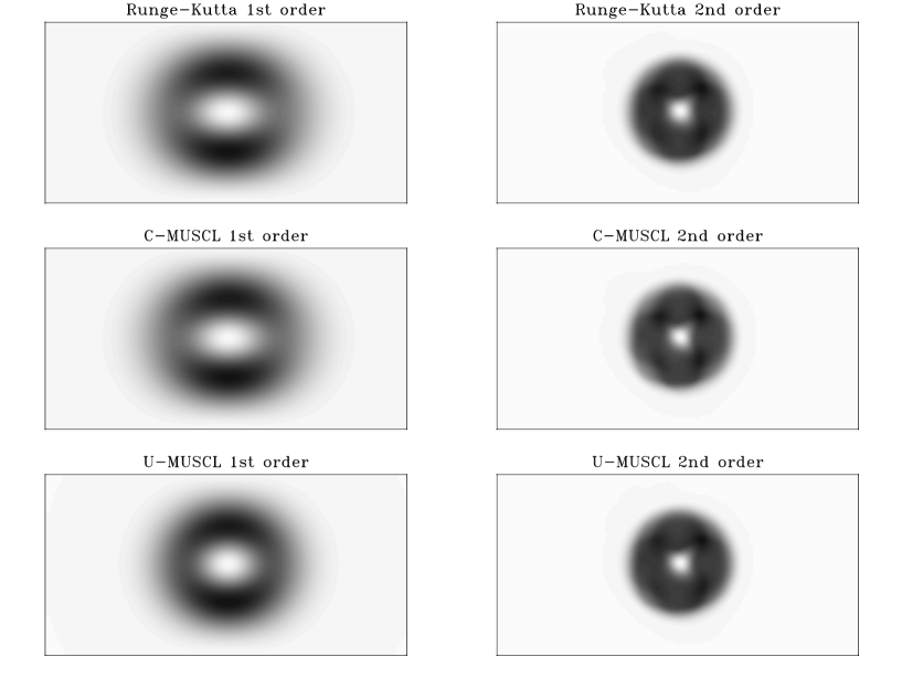
Figure 3: Magnetic loop advection test for a Cartesian grid with $n_{x}=128$ and $n_{y}=64$: each panel shows a gray-scale image of the magnetic energy ($B_{x}^{2}+B_{y}^{2}$) at time $t=2$. The scheme used to compute each image is provided in the title of each panel. Second-order schemes give very similar results, while the first order U-MUSCL scheme performs slightly better than the two other first order schemes.

Figure 4: Magnetic energy as a function of time for the field loop advection test. The upper solid line is the solution for perfect advection. The lower lines are for the first order schemes: Runge-Kutta (dotted line), C-MUSCL (dashed line) and U-MUSCL (solid line). Runge-Kutta and C-MUSCL results are indistinguishable in this case. The 3 intermediate lines correspond to second order schemes and use the same line convention. The dot-dashed lines is the AMR result obtained with U-MUSCL and using $\ell_{min}=3$ and $\ell_{max}=9$.

Let us first focus our attention on a simple test of pure advection which was recently proposed by Gardiner and Stone (2005) to investigate the advection properties of their CT scheme. It consists in the advection of a magnetic field loop with a uniform velocity field. It is of particular relevance in our case, since we are dealing with kinematic induction problems. The computational domain is defined by $-1<x<1$ and $-0.5<y<0.5$. The boundary conditions are periodic. The flow velocity is set to $u=2$, $v=1$ and $w=0$.

The initial magnetic field is such that $B_{z}=0$, while $B_{x}$ and $B_{y}$ are defined using the z-component of the potential vector A (with $\hbox{\bf B}=\mbox{\boldmath$\nabla$}\times\hbox{\bf A}$), as an axisymmetric function of the form

$$A_{z}=\left\{\begin{array}[]{cc}R-r&\rm{for~{}}r<R\,,\\ 0&\rm{otherwise}\,,\end{array}\right.$$ (50)

with $R=0.3$ and $r=\sqrt{x^{2}+y^{2}}$. The exact amplitude of the magnetic field is arbitrary, since we are solving a linear equation, we used $B=1$. In the following, we use exactly the same resolution as Gardiner and Stone (2005).

We perform the numerical integration of the induction equation up to time $t=2$ with a Courant factor see (34) is equal to $0.8$, for which the magnetic loop has evolved twice across the computing box. Our first set of runs use a regular Cartesian grid with $N_{x}=128$ and $N_{y}=64$. We test the three different schemes, to first order (slope limiters were set to zero) and to second order. The aim here is to estimate the numerical diffusion of our various schemes.

Figure 3 shows gray-scale images of the magnetic energy $B_{x}^{2}+B_{y}^{2}$ for the six runs. Maximum field dissipation occurs at the center and boundaries of the loop where the current density is initially singular. Second order schemes all give very similar results. At first order, the U-MUSCL scheme performs slightly better than the other two, with a more isotropic pattern. To estimate more quantitatively the numerical diffusion, we have plotted in Figure 4 the total magnetic energy in the computational box as a function of time. Perfect advection would have given a constant value of $E_{tot}=\pi R^{2}$. As expected, first order schemes are much more diffusive than the second order ones. All the latter give almost identical results, Runge-Kutta being the most diffusive, followed by C-MUSCL and then U-MUSCL. At first order, the U-MUSCL scheme also appears less diffusive than the two other schemes.

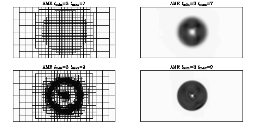
Figure 5: Magnetic loop advection test: AMR result with the U-MUSCL scheme. The two upper plots are for $\ell_{max}=7$, while the two lower plots are for $\ell_{max}=9$. The right panels show gray-scale images of the magnetic energy, while the left panels show the AMR grid (only “oct” boundaries are shown for clarity, but each oct is in fact subdivided into 4 children cells).

We now present the results obtained with our AMR implementation using the U-MUSCL scheme (C-MUSCL giving almost identical results). We start with a base Cartesian grid with $N_{x}=8$ and $N_{y}=4$, corresponding to $\ell_{min}=3$. It is then adaptively refined up to $\ell_{max}$, using the following refinement criterion on the magnetic energy $E=B_{x}^{2}+B_{y}^{2}$

$$\frac{\max{\left(\left|\Delta_{x}E\right|,\left|\Delta_{y}E\right|\right)}}{E+0.01}>0.05\,.$$ (51)

With this criterion, each cell for which the change of local magnetic energy exceeds 5% of the local magnetic energy is refined. The first test is done with $\ell_{max}=7$, in order to reach the same spatial resolution as the previous simulations with a $128\times 64$ Cartesian grid. The magnetic energy map at $t=2$ is shown in Figure 5, together with a line plot showing the corresponding AMR grid. In this last plot, only “oct” boundaries are shown for clarity (each oct is in fact subdivided into four children cells). We conclude that the AMR results are indistinguishable from the equivalent resolution Cartesian run, but the computational cost is lower: at time $t=2$, the total number of leaf cells in the AMR tree is $3149$. This is to be compared with the number of cells in a Cartesian grid equivalent to the finer resolution which would be $128\times 64=8129$.

In order to illustrate more convincingly the interest of using an AMR grid in this case, we have performed the same simulation with now $\ell_{max}=9$. The magnetic energy map and the corresponding AMR grid are shown in Figure 5. Refinements are now much more localized at the center and boundaries of the magnetic loop. Numerical diffusion has dramatically decreased, as shown on Figure 4, where the time history of the total magnetic energy is plotted. The agreement with the ideal case has improved substantially. The total number of cells at $t=2$ is now $16433.$ This is only a factor of 2 greater than the previous Cartesian runs, but a factor of 8 lower than the Cartesian grid equivalent to the finer resolution $512\times 256=131072$.

4.2 The Ponomarenko Dynamo

One of the simplest known dynamo flows, and the one we will start our investigation with, is the Ponomarenko dynamo (Ponomarenko, 1973). The geometry of the flow is remarkably simple. In cylindrical polar coordinates $(s,\phi,z)$, it is

$$\hbox{\bf v}=\left\{\begin{array}[]{ll}(0,s\Omega,u_{z})\mbox{\ \hskip 28.45274pt\ }&\mbox{for\ }s\leq s_{0}\,,\\ \mbox{\boldmath$0$}&\mbox{for\ }s>s_{0}\,.\end{array}\right.$$ (52)

This flow features an abrupt discontinuity across the cylinder at $s=s_{0}$, such discontinuity yields an intricate behavior in the limit $\mbox{Rm}\rightarrow\infty$. The growth rate remains constant in this limit, but the flow does not qualify as a proper fast dynamo, for the critical eigenmode keeps changing with Rm (see Childress and Gilbert, 1995). Variants of this flow, known as “smoothed Ponomarenko flows” introduce a typical length scale over which the flow vanishes, and can help circumvent this difficulty (Gilbert, 1988). We will however consider here the original Ponomarenko flow with an abrupt discontinuity. Since the flow is discontinuous, an explicit physical resistivity (associated with a finite value of the Reynolds number Rm) is essential in setting the typical lengthscale of the magnetic field ($\ell\sim\mbox{Rm}^{-1/2}$).

As with most dynamo problems, numerical resolution is classically achieved using spectral expansions (e.g. Childress and Gilbert, 1995). We use here our numerical approach to validate our scheme as well as to test the properties of the AMR implementation and its ability to deal with a discontinuous input flow. Because of the cylindrical nature of the flow, it is natural to think of adapting the scheme to this system of coordinates. We have therefore written a cylindrical version of our algorithm (note however that AMR has not been implemented in this version of the code). The discontinuity at $s=s_{0}$ correspond exactly to a cell boundary. It is important to appreciate that there is no flow along the $s$ direction with this approach. This implies that numerical diffusion vanishes in this direction. It is only nonzero in the $\phi$ and $z$ directions. This emphasizes the importance of physical resistivity to obtain meaningful results.

In most practical work, sharp structures in the flow can occur which are not necessarily aligned with the grid (see for example the next application). We will therefore solve this same dynamo problem using also a Cartesian grid. A very large resolution is needed in order to reach a fine discretisation of the cylinder at $s=s_{0}$ (around which the field is localized over a lengthscale $\ell\sim\mbox{Rm}^{-1/2}$). This will be achieved using our AMR approach.

The Ponomarenko flow can be investigated analytically (Ponomarenko, 1973). Such an analysis reveals that an exponentially growing solution in time can be obtained for $\mbox{Rm}=Us_{0}/\eta\geq\mbox{Rm}_{c}\simeq 17.7$ (where $U=\sqrt{\Omega^{2}s_{0}^{2}+u_{z}^{2}}$). This is obtained using a spectral expansion of the variables in $z$ and $\phi$ of the form $\exp(im\phi+ikz)$. The most unstable mode (at $\mbox{Rm}=\mbox{Rm}_{c}$) corresponds to $u_{z}=1.3\,\Omega s_{0}$, $m=1$ and $k_{c}\,s_{0}=0.39$. For larger magnetic Reynolds number, other modes become unstable.

Figure 6: Growth rate for the Ponomarenko dynamo as a function of the magnetic Reynolds number. The solid curve corresponds to the first unstable mode, and the dotted line to its harmonic $k=2\times k_{c}$ . For both modes, the growth rate first increases and then decreases with Rm (as expected from analytical linear theory). As the Reynolds number increases, a transition occurs from $k_{c}$ to $2\times k_{c}$ . The star symbol $\mbox{Rm}=400$ corresponds to the AMR simulation.

Using the cylindrical version of our code, we have numerically calculated the magnetic energy growth rates for the Ponomarenko flow for a large range of magnetic Reynolds numbers, going from $Rm=16.7$ to $Rm=2000$.

We use $s_{0}$ as unit of length, thus senting $s_{0}\equiv 1$. The grid extends from $0.2$ to $3.5$ in radius and the azimuthal coordinate cover the full $2\pi$ range. The resolution of the grid is $(N_{r},N_{\phi},N_{z})=(64,50,64)$. For the vertical extent of the computational domain $L_{\rm box}$, we consider two different cases: case I, for which $L_{\rm box}=2\pi/k_{g}$, with $k_{g}$ being $0.39$ and case II for which $k_{g}=0.78$. Let us recall that the classical numerical approach for this problem relies on a Fourier expansion in $z$. In this case, a single mode $k$ is retained in $z$ to enlighten the numerical procedure, the optimal value of $k_{c}$ being obtained after optimization. Our numerical approach does not allow this sort of mode selection. Instead, we can only fix the $z$-periodicity of the computational box. In case I, $L_{\rm box}$ was chosen to match the wavelength of the most unstable mode. However, harmonics of the critical mode, being unstable for large Reynolds numbers, can also develop in the computational box (as can be seen for example in the figure $6.4$ of Plunian and Massé, 2002). This is a known issue, which only occurs here because the calculation is not restricted to a single mode in $z$.

The transition from the first unstable mode to a higher mode in $z$ occurs for Reynolds numbers twice critical. We have been able to follow the first unstable mode to Reynolds number larger than the transition to $k=2\times k_{c}$ by carefully selecting the initial condition (and restricting to short enough time integrations). We have also turned our attention to the $k=2\times k_{c}$ instability below the transition by studying a computational box of half the standard size in the $z$-direction. The resulting diagram is presented in figure 6 .

When $Rm=16.7$, the growth rate $\sigma$ of the magnetic energy was found to be negative, as expected. For $Rm\in[17.7,20]$ $\sigma$ becomes positive in case I and the eigenmode corresponds to $k=k_{c}$ . When $Rm=20$, it is characterized by $m=1$, $k=k_{c}=0.39$ and $\sigma=3.4\times 10^{-3}$. This is in very good agreement with linear theory (Ponomarenko, 1973). The growth rate obtained for larger $Rm$ is represented by the solid line on figure 6.

In case II, we use a computational domain with half the vertical extend of case I. The growing mode has different properties. It is characterized by $m=1$ and $k=2\times k_{c}=0.78$. Its growth rate as a function of $Rm$ is shown on figure 6 using the dotted line. The transition between both modes is clear near $\mbox{Rm}\simeq 30$. Unless the initial conditions are carefully chosen and the time integration is short enough, the mode $k=2\times k_{c}$ will overcome the first critical mode for $\mbox{Rm}>30$ .

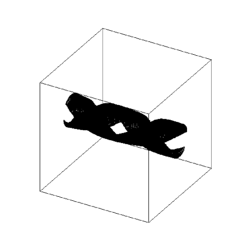
Figure 7: Ponomarenko dynamo with $\mbox{Rm}=400$. Left panel: surface of isovalue $B^{2}/2=10^{6}$ for the magnetic energy density at time $t=200$. Right panel: mesh geometry (for clarity, only “octs” boundaries are displayed here).

In order to validate the AMR implementation, we have also performed simulations on a Cartesian grid with $\mbox{Rm}=400$. The size of the box is $L_{\rm box}=2\pi/0.78$, similar to case II described above. For this run, we took $\ell_{\rm min}=5$ and $\ell_{\rm max}=8$, which has yield a maximum of $751360$ cells on the grid (this is a factor of $22$ smaller than the number of cells of a $256^{3}$ uniform grid). The refinement strategy was based on the magnitude of the velocity gradient. The growth rate of the magnetic energy in this case was measured to be $\sigma_{\rm AMR}=0.0562$ (see the star represented in figure 6). This is in very good agreement with the value $\sigma=0.0542$ obtained with the cylindrical version of the code for the same parameter set.

The structure of the growing eigenmode in this simulation is illustrated in figure 7. The left panel represents surfaces of isovalue of the magnetic energy density $B^{2}/2$ at $t=200$ while the structure of the AMR grid is illustrated on the right panel. The grid is only refined at the sharp boundary between the inner rotating cylinder and the outer motionless medium. This simulation demonstrates both the ability of the scheme to simulate the Ponomarenko dynamo using a Cartesian grid and the possibility to handle discontinuities in the flow which are not aligned with the grid.

4.3 The ABC Dynamo

We now consider another dynamo flow, known as the ABC-flow (for Arnold-Beltrami-Childress). It is defined by a periodic flow

$$\hbox{\bf u}=A\,(0,\sin x,\cos x)+B\,(\cos y,0,\sin y)+C\,(\sin z,\cos z,0)\,.$$ (53)

We limit our attention here to the classical case of $(A:B:C)=(1:1:1)$. Let us stress that this test is fully 3D and requires a significant computational effort.

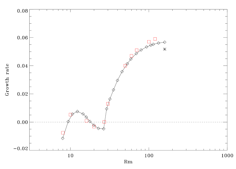
Figure 8: Growth rate for the ABC dynamo as a function of the magnetic Reynolds number. This diagram agrees remarkably well with the results obtained using a spectral description by Galloway and Frisch 1986 (shown as boxes). The star is obtained with the AMR implementation.

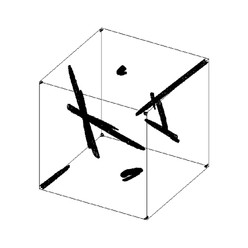
Figure 9: ABC dynamo investigated with the AMR strategy at $\mbox{Rm}=159$. On the left panel: surface of isovalue of the magnetic energy density $B^{2}/2=3\times 10^{19}$ at time $t=80$; on the right panel: the AMR mesh geometry (for clarity, only “octs” boundaries are displayed here).

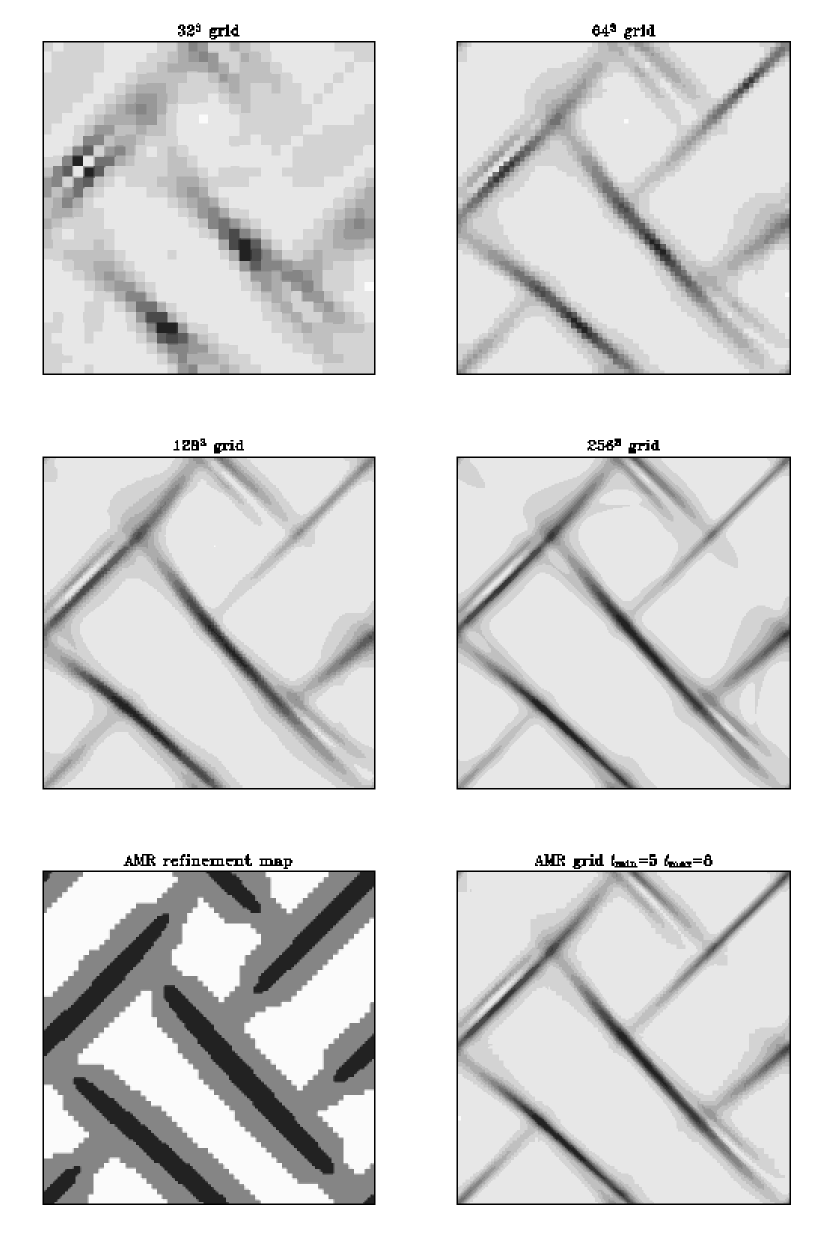
Figure 10: The ABC dynamo is investigated at $\mbox{Rm}=159$ with various resolutions. The projected magnetic energy density is represented for each run. The convergence is demonstrated on the Cartesian grid and the ability of the AMR grid to capture the solution is assessed.

This flow is known as a fast-dynamo: at large, but finite, $Rm$, eigenmodes in the form of cigar-shaped structures develop (e.g. Childress and Gilbert, 1995). They are very localized in space (again $\ell\sim\mbox{Rm}^{-1/2}$), therefore constituting ideal candidates for a investigation using the AMR methodology. Traditionally, these problems have been modeled using spectral methods (e.g. Galloway and Frisch, 1986). The choice of the velocity profile in the form of Fourier modes was largely guided by the underlying numerical method. More recently, Archontis et al. (2003) have investigated this flow using a staggered grid and array valued functions.

We want to emphasize here that because we are now investigating dynamo action at large Rm, the stability properties of the Godunov scheme will be essential. This will be particularly true using an AMR grid. The refinement strategy will ensure that the physical resistivity dominates on the finer grid which is centered around the cigar shaped magnetic structures (using a threshold on $\mid\mid\hbox{\bf B}\mid\mid$). Regions relying on a coarser grid, however, will be dominated by the numerical resistivity. The properties of the scheme, both in terms of stability and of low numerical resistivity are therefore essential ingredients to the success of the AMR methodology.

Dynamo action associated with this flow is not at all trivial. There are at least two regions of instability in the parameter space, one for $8.9\leq\mbox{Rm}\leq 17.5$ and a second for $\mbox{Rm}\geq 27$ (see Galloway and Frisch, 1986). This second instability has been followed up to Rm of a few thousand. We plan to use our methodology to investigate higher values of Rm in the near future. This intricate behavior of the growth rate with Rm suggests the use of high enough values of the magnetic Reynolds number for convergence study. Otherwise, an increase of the resisitivity (decrease in Rm) could yield an increase in the growth rate by sampling different regions of instability.

As in the case of the Ponomarenko dynamo, we have calculated the growth rate as a function of Rm. The corresponding graph, using a Cartesian grid with $(N_{x},N_{y},N_{z})=(128,128,128)$ is presented on figure 8 . This diagram is in excellent agreement with the spectral results of Galloway and Frisch, 1986, shown in the same figure as squares.

We now investigate this dynamo using the AMR scheme. We want to stress that using AMR without care for such problems is not free of risk, the grid being affected by the solution and vice versa. Although for both the advection and Ponomarenko tests, the solution has been well captured using straightforward refinement criteria, the situation is more subtle for the ABC flow, for which the field generation is not localized. If the strategy is not adequate, some regions of the flow might not be refined as they should be, and thus be subject to a large amount of numerical diffusivity. The choice of the optimal refinement strategy for the ABC flow is beyond the scope of the present study. It could for example be based on various flow properties, such as Liapunov exponents, stagnation points, etc, or on various field properties, such as gradients, truncation errors, etc.

As a first step, we have used here a criterion based on the magnetic energy density which allows the grid to be easily densified near the cigar-like structures: when the local magnetic energy density on level 5, 6, 7… is respectively greater than 4, 16, 64… times the mean energy density, new refinements are triggered. This strategy is best applied at large Rm for which the magnetic structures are well localized. We focus here on $\mbox{Rm}=159\,\,(=1000/2\pi)$.

The AMR simulation yields a growth rate of $0.052$ after $77$ hours of wall–time computing using $8$ processors. It is evolved until $t=80$. At that time, the grid is composed of $455659$ cells. The structure of the eigenmode and the topology of the grid are illustrated in figure 9. For comparison, the Cartesian grid simulation with $256^{3}$ cells yields a growth rate of $0.055$ but requires $138$ hours to evolve the solution only up to $t=46$ and using $64$ processors! The AMR simulation has therefore allowed a gain in memory of a factor of $37$, and a speed-up of $25$ in time. All our computations are compared on figure 10. The first four panels show the projected magnetic energy obtained varying the resolution from $32^{3}$ to $256^{3}$. Computations performed with $128^{3}$ and $256^{3}$ cells reveal very little differences and clearly indicate convergence. The two bottom snapshots illustrates the structure of the grid in the AMR simulations (left panel) and the projected magnetic energy (right panel). There is a good agreement between the AMR simulation and the run performed on the $256^{3}$ grid (about $10\%$).

5 Conclusions and perspectives

We have shown that the Constrained Transport approach for preserving the solenoidal character of the magnetic field could be combined with a Godunov method, provided a two-dimensional Riemann solver can be used. We have further shown how this could be combined with a MUSCL high order scheme. We considered three schemes for the predictive step, each with its own merits. For a uniform velocity field, these CT schemes are strictly equivalent to well known finite volume schemes on the staggered grid. This important result provides additional support to the advection properties of the CT framework.

We have implemented this strategy on a kinematic dynamo problem, for which only the induction equation needs to be considered. We have shown that the Godunov framework allows an efficient AMR treatment of fast dynamos, by ensuring the numerical stability of the scheme in regions solved with a coarse grid (for which the effects of the physical diffusion are vanishing).

The approach introduced here clearly needs to be adapted to the full set of MHD equations, for which solving the Riemann problem is no longer a trivial task. This important step raises several additional difficulties and is the object of a forthcoming paper (Fromang et al. (2006)).

References

- Archontis et al. (2003) Archontis, V., Dorch, S. B. F., Nordlund, A., Jan. 2003. Numerical simulations of kinematic dynamo action. Astronomy & Astrophysics 397, 393–399.
- Balsara (2001) Balsara, D. S., 2001. Divergence-free adaptive mesh refinement for magnetohydrodynamics. J. Comput. Phys. 174 (2), 614–648.
- Balsara and Spicer (1999) Balsara, D. S., Spicer, D. S., 1999. A staggered mesh algorithm using high order Godunov fluxes to ensure solenodial magnetic fields in magnetohydrodynamic simulations. J. Comput. Phys. 149 (2), 270–292.
- Berger and Colella (1989) Berger, M. J., Colella, P., May 1989. Local adaptive mesh refinement for shock hydrodynamics. Journal of Computational Physics 82, 64–84.
- Berger and Oliger (1984) Berger, M. J., Oliger, J., 1984. Adaptive mesh refinement for hyperbolic partial differential equations. J. Comp. Phys. 53, 484–512.
- Bouchut (2005) Bouchut, F., 2005. Non-linear Stability of Finite Volume Methods for Hyperbolic Conservation Laws. Frontiers in Mathematics, Birkhäuser.
- Brackbill and Barnes (1980) Brackbill, J. U., Barnes, D. C., May 1980. The effect of nonzero product of magnetic gradient and B on the numerical solution of the magnetohydrodynamic equations. Journal of Computational Physics 35, 426–430.
- Childress and Gilbert (1995) Childress, S., Gilbert, A. D., 1995. Stretch, Twist, Fold. The Fast Dynamo, XI, 406 pp.. Springer-Verlag Berlin Heidelberg New York. Also Lecture Notes in Physics, volume 37.
- Christensen et al. (2001) Christensen, U. R., Aubert, J., Cardin, P., Dormy, E., Gibbons, S., Glatzmaier, G. A., Grote, E., Honkura, Y., Jones, C., Kono, M., Matsushima, M., Sakuraba, A., Takahashi, F., Tilgner, A., Wicht, J., Zhang, K., Dec. 2001. A numerical dynamo benchmark. Physics of the Earth and Planetary Interiors 128, 25–34.
- Colella (1990) Colella, P., 1990. Multidimensional upwind methods for hyperbolic conservation laws. J. Comput. Phys. 87 (1), 171–200.
- Crockett et al. (2005) Crockett, R. K., Colella, P., Fisher, R. T., Klein, R. I., McKee, C. F., 2005. An unsplit, cell-centered godunov method for ideal mhd. Journal of Computational Physics 203, 422–448.
- Dedner et al. (2002) Dedner, A., Kemm, F., Kröner, D., Munz, C. D., Schnitzer, T., Wesenberg, M., 2002. Hyperbolic Divergence Cleaning for the MHD Equations. Journal of Computational Physics 175, 645–673.
- Evans and Hawley (1988) Evans, C. R., Hawley, J. F., Sep. 1988. Simulation of magnetohydrodynamic flows - A constrained transport method. The Astrophysical Journal 332, 659–677.
- Fromang et al. (2006) Fromang, S., Hennebelle, P., Teyssier, R., 2006. An MHD version of the AMR high order Godunov code RAMSES. Astronomy & Astrophysics , in prep. .
- Galloway and Frisch (1986) Galloway, D. J., Frisch, U., 1986. Dynamo action in a family of flows with chaotic streamlines. Geophys. Astrophys. Fluid Dynamics 36, 53–83.
- Gardiner and Stone (2005) Gardiner, T. A., Stone, J. M., May 2005. An unsplit Godunov method for ideal MHD via constrained transport . Journal of Computational Physics 205, 509–539.
- Gilbert (1988) Gilbert, A., 1988. Fast dynamo action in the Ponomarenko dynamo. Geophys. Astrophys. Fluid Dyn. 44, 241–258.
- Harder and Hansen (2005) Harder, H., Hansen, U., May 2005. A finite-volume solution method for thermal convection and dynamo problems in spherical shells. Geophysical Journal International 161, 522–532.
- Khokhlov (1998) Khokhlov, A. M., 1998. Fully threaded tree algorithms for adaptive refinement fluid dynamics simulations. J. Comput. Phys. 143 (2), 519–543.
- Kleimann et al. (2004) Kleimann, J., Kopp, A., Fichtner, H., Grauer, R., Germaschewski, K., Mar. 2004. Three-dimensional MHD high-resolution computations with CWENO employing adaptive mesh refinement. Computer Physics Communications 158, 47–56.
- Kravtsov et al. (1997) Kravtsov, A. V., Klypin, A. A., Khokhlov, A. M., Jul. 1997. Adaptive Refinement Tree: A New High-Resolution N-Body Code for Cosmological Simulations. The Astrophysical Journal Supplement Series 111, 73–+.
- Li and Li (2004) Li, S., Li, H., 2004. A novel approach of divergence-free reconstruction for adaptive mesh refinement. J. Comput. Phys. 199 (1), 1–15.
- Londrillo and Del Zanna (2000) Londrillo, P., Del Zanna, L., Feb. 2000. High-Order Upwind Schemes for Multidimensional Magnetohydrodynamics. The Astrophysical Journal 530, 508–524.
- Londrillo and Del Zanna (2004) Londrillo, P., Del Zanna, L., Mar. 2004. On the divergence-free condition in Godunov-type schemes for ideal magnetohydrodynamics: the upwind constrained transport method. Journal of Computational Physics 195, 17–48.
- Matsui and Okuda (2005) Matsui, H., Okuda, H., 2005. MHD dynamo simulation using the GeoFEM platform - verification by the dynamo benchmark test. International Journal of Computational Fluid Dynamics 19, 15–22.
- Plunian and Massé (2002) Plunian, F., Massé, P., 2002. Couplage magnétohydraulique: modélisation de la dynamo cinématique (pp. 215–247), in Electromagnétisme et éléments finis, 3, Ed. Meunier G. Hermes.
- Ponomarenko (1973) Ponomarenko, Y., 1973. On the theory of hydromagnetic dynamos (English translation). J. Appl. Mech. Tech. Phys. 14, 775–778.
- Popinet (2003) Popinet, S., 2003. Gerris: a tree-based adaptive solver for the incompressible euler equations in complex geometries. J. Comput. Phys. 190 (2), 572–600.
- Powell et al. (1999) Powell, K. G., Roe, P. L., Linde, T. J., Gombosi, T. I., De Zeeuw, D. L., 1999. A Solution-Adaptive Upwind Scheme for Ideal Magnetohydrodynamics. Journal of Computational Physics 154, 284–309.
- Ryu et al. (1998) Ryu, D., Miniati, F., Jones, T. W., Frank, A., Dec. 1998. A Divergence-free Upwind Code for Multidimensional Magnetohydrodynamic Flows. The Astrophysical Journal 509, 244–255.
- Samtaney et al. (2004) Samtaney, R., Jardin, S. C., Colella, P., Martin, D. F., Dec. 2004. 3D adaptive mesh refinement simulations of pellet injection in tokamaks. Computer Physics Communications 164, 220–228.
- Teyssier (2002) Teyssier, R., Apr. 2002. Cosmological hydrodynamics with adaptive mesh refinement. A new high resolution code called RAMSES. Astronomy & Astrophysics 385, 337–364.
- Toro (1999) Toro, E., 1999. Riemann Solvers and Numerical Methods for Fluid Dynamics. Springer-Verlag.
- Tóth (2000) Tóth, G., 2000. The =0 Constraint in Shock-Capturing Magnetohydrodynamics Codes. Journal of Computational Physics 161 (2), 605–652.
- Tóth and Roe (2002) Tóth, G., Roe, P. L., 2002. Divergence- and curl-preserving prolongation and restriction formulas. J. Comput. Phys. 180 (2), 736–750.
- van Leer (1977) van Leer, B., 1977. Towards the ultimate conservative difference scheme: IV. A new approach to numerical convection. Journal of Computational Physics 23, 276–299.
- Yee (1966) Yee, K., 1966. Numerical solution of initial boundary value problems involving Maxwell equations in isotropic media. IEEE Trans. Antenna Propagation 302.
- Ziegler (1999) Ziegler, U., Jan. 1999. A three-dimensional Cartesian adaptive mesh code for compressible magnetohydrodynamics. Computer Physics Communications 116, 65–77.