Interacting galaxies and cosmological parameters

We propose a (physical)-geometrical method to measure $\Omega_{m\circ}$ and $\Omega_{\Lambda\circ}$, the present rates of the density cosmological parameters for a Friedmann-Lemaître universe. The distribution of linear separations between two interacting galaxies, when both of them undergo a first massive starburst, is used as a standard of length. Statistical properties of the linear separations of such pairs of “interactivated” galaxies are estimated from the data in the Two Degree Field Galaxy Redshift Survey. Synthetic samples of interactivated pairs are generated with random orientations and a likely distribution of redshifts. The resolution of the inverse problem provides the probability densities of the retrieved cosmological parameters. The accuracies that can be achieved by that method on $\Omega_{m\circ}$ and $\Omega_{\Lambda\circ}$ are computed depending on the size of ongoing real samples. Observational prospects are investigated as the foreseeable surface densities on the sky and magnitudes of those objects.

1 Introduction

Variation in the scale factor $R(t)$ of a Friedmann-Lemaître (FL) universe with cosmic time $t$ affects the observable relations $m\longleftrightarrow z_{c}$ and $\theta\longleftrightarrow z_{c}$ between apparent magnitude $m$ and angular size $\theta$ versus the cosmological redshift $z_{c}$ of standard sources. When possible, a solution to the inverse problem may then supply the whole story of $R(t)$ and the spatial curvature.

The $m\longleftrightarrow z_{c}$ relation provided the first estimation of the expansion rate $H\buildrel{def}\over{=}\dot{R}/R$ (Lemaître Lem27 (1927)), a long time ago. Much more recently, supernovae SNIa (Riess et al. Riess98 (1998), Perlmutter et al. Perlm99 (1999)) were the standard candles that accredited – with the help of the angular power spectrum of the anisotropy for the Cosmic Microwave Background Radiation (CMBR) – the so-called “concordance model” in which the density parameters for cold matter ($\Omega_{m}\buildrel{def}\over{=}8\pi G\rho_{m}/3H^{2}$) and for cosmological constant ($\Omega_{\Lambda}\buildrel{def}\over{=}\Lambda c^{2}/3H^{2}$) have the present (index_∘) values $\Omega_{m\circ}\sim 1/3$ and $\Omega_{\Lambda\circ}\sim 2/3$. All this revived a dominant $\Omega_{\Lambda\circ}$ universe, after Lemaître (Lem27 (1927), Lem31 (1931)). But as pointed out by Blanchard et al (Blan03 (2003)), that concordance is not entirely free from weak hypotheses, and those authors argued that the previously dominant Einstein-de-Sitter model ($\Omega_{m}=1$ and $\Omega_{\Lambda}=0$) was still not excluded by available data.

The case for $\Omega_{\Lambda\circ}$ is important. That parameter is not only determinant for the geometrical age of the universe and for the evolution of large structures but, in the FL equations on the scale factor $R(t)$, the geometrical cosmological constant $\Lambda$ may be, at least formally and partly or totally, exchanged with a physical “vacuum energy”, a perfect and Lorentz invariant fluid of equation of state $p=w\rho c^{2}$ with $w_{\Lambda}=-1$ and $\rho_{\Lambda}=\Lambda c^{2}/4\pi G$ (Lemaître Lem34 (1934)) that this author judged to be “essentially the meaning of the cosmical constant”. And the cosmological tests that detected $\Omega_{\Lambda\circ}\not=0$ may also be used to constrain the $w\not=-1$ or $w\not=constant$ of more elusive fluids like dark energy or quintessence.

To that purpose the $\theta\longleftrightarrow z_{c}$ relation is also a promising cosmological test that was first investigated by Tolman (Tol30 (1930)). If an object has a projected linear separation $PS$ on the plane of the sky at the time of emission $t_{e}$, the radial motion of received photons leads to an observed angular size:

$$\theta_{\circ}(z_{c})=\frac{PS\ (1+z_{c})}{d}\buildrel{def}\over{=}\frac{PS}{d_{A}}\ \ .$$ (1)

In the above expression, $d$ is the “metric” or “comoving tranverse” or “proper motion” “distance” of the source and $d_{A}$ is its “angular size–distance”. The expressions for $d$ are obtained by intregration of the radial light’s movement from the source to the observer ($d_{-}$, $d_{f}$, $d_{+}$ respectively are for negative, null, and positive curvatures of space, $\Omega_{r}$ is the density parameter of radiation, and $\Omega_{k}\buildrel{def}\over{=}-kc^{2}/R^{2}H^{2}$ is the reduced curvature of space related to other $\Omega_{i}$ by $\Omega_{m}+\Omega_{r}+\Omega_{\Lambda}+\Omega_{k}=1$) :

$$d_{-}=\frac{c}{H_{\circ}\mid\Omega_{k\circ}\mid^{\frac{1}{2}}}\ \sinh\left[\mid\Omega_{k\circ}\mid^{\frac{1}{2}}F(z_{c})\right]\ \ \ (H^{3}\ \rm{space})$$ (2)

$$d_{f}=\frac{c}{H_{\circ}}\ F(z_{c})\ \ \ (E^{3}\ \rm{space})$$ (3)

$$d_{+}=\frac{c}{H_{\circ}\mid\Omega_{k\circ}\mid^{\frac{1}{2}}}\ \sin\left[\mid\Omega_{k\circ}\mid^{\frac{1}{2}}F(z_{c})\right]\ \ \ (S^{3}\ \rm{space})$$ (4)

with

$$\begin{array}[]{l}\displaystyle{F(z_{c})=\int_{0}^{z_{c}}[\Omega_{r\circ}(1+x)^{4}+\Omega_{m\circ}(1+x)^{3}}\\ \ \ \ \ \ \ \ \ \ \ \ \ \ \ \ \ \ \ \ \ \ \ \ \ \ \ +\Omega_{k\circ}(1+x)^{2}+\Omega_{\Lambda\circ}]^{-\frac{1}{2}}\ dx\ \ \ .\end{array}$$ (5)

We note that the $\theta_{\circ}\longleftrightarrow z_{c}$ relation is not directly linked to the projected separation $PS$ but to the product $H_{\circ}\cdot PS$, if the observational determination of real $PS$ uses – and is then inversely proportional to – the rate of $H_{\circ}$, i.e. when distances are deduced from redshifts and not directly from indicators.

The discriminating power of the $\theta_{\circ}\longleftrightarrow z_{c}$ relation versus some sets of cosmological parameters is displayed in Fig. 1. For currently favoured cosmological models, $\theta_{\circ}$ remains greater than a minimum value :

$$\theta_{\circ}(\arcsec)>\frac{PS(kpc)}{10}\ \ \ .$$ (6)

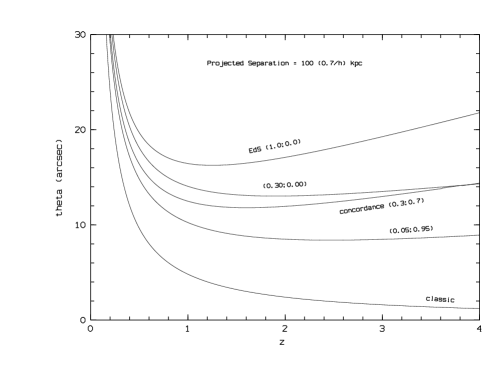
Figure 1: Sensitivity of the $\theta_{\circ}\longleftrightarrow z_{c}$ relation to $\Omega_{m\circ}$ and $\Omega_{\Lambda\circ}$.

Attempts to constrain the cosmological parameters with the $\theta_{\circ}\longleftrightarrow z_{c}$ relation have been performed. First conclusive results with radio-sources have been suggested by Kellermann (Kell93 (1993)) for the deceleration parameter $q_{\circ}$ ($q=\Omega_{r}+\Omega_{m}/2-\Omega_{\Lambda}$ and $q_{\circ}\approx\Omega_{m\circ}/2-\Omega_{\Lambda\circ}$ in our expanded universe). As reviewed by Gurvits et al. (Gurv99 (1999)), the large radio structures had supplied inconclusive or paradoxical data : classical $\theta_{\circ}\propto 1/z$ or even $\theta_{\circ}\sim$ constant! Those authors did focus on milliarcsec compact radio sources, which are presumably physically very young so not very related to or affected by the cosmic evolution of the intergalactic medium. They derived a constraint in that way on the deceleration parameter $q_{\circ}=0.21\pm 0.30$. Guerra et al. (Guerra00 (2000)) have obtained wide contours in the ($\Omega_{m\circ}$, $\Omega_{\Lambda\circ}$) plane with 20 powerful double-lobed radio galaxies as yardsticks. Lima & Alcaniz (Lima02 (2002)) and Chen & Ratra (Chen03 (2003)), using the data of Gurvits et al. (Gurv99 (1999)), have both derived wide constraints on the densities parameters and also on the index in the expression of the potential of the dark energy scalar field, which could challenge $\Lambda$. Zhu & Fujimoto (Zhu02 (2002)) with the data of Gurvits et al. (Gurv99 (1999)), Zhu et al. (Zhu04b (2004)) using the data of Guerra et al. (Guerra00 (2000)), and Zhu & Fujimoto (Zhu04 (2004)) also investigated the $\theta_{\circ}\longleftrightarrow z_{c}$ relation to constrain the $w$ parameter of dark energy and the free parameters of non-standard cosmologies.

The main problems encountered with astrophysical objects – or non-interacting pairs – in the cosmological utilization of their $\theta_{\circ}(z_{c})$ relation are:

• i) the statistical evolution of linear size with cosmic time (and then with $z_{c}$) as already mentioned for radio sources. This is well known for the clusters of galaxies whose relaxation time is comparable to the Hubble time ($H_{\circ}^{-1}$) and which are still accreting material in the central parts of superclusters. The more recent discovery that the bulk of galaxies are the result of multiple merging processes seems to exclude them for that purpose. As the intergalactic medium IGM is also evolving with cosmic time, the selection of very young (unmerged) galaxies does not seem to be a solution.

• ii) measurement biases due to fuzzy intrinsic photometric profiles of objects (galaxies, clusters of galaxies) and to the fast decrease in surface brightness with redshift.

• iii) redshifts 2 to 3 have to be reached to disentangle the partial degeneracy between $\Omega_{m\circ}$ and $\Omega_{\Lambda\circ}$.

With the purpose of avoiding the most important part of those drawbacks, our idea is to replace the standard objects by pairs of bright related objects. Physically this consists in finding pairs of objects displaying a special feature because they are at a characteristic physical distance from each other. Replacing diffuse objects by pairs of point-like (or relatively well “picked”) sources removes observational bias in the measure of $\theta_{\circ}$. If the physical process that causes the special feature is not sensitive to the cosmic evolution, the main drawback of the method is removed. If the objects furthermore have strong emission lines, measuring their redshift becomes obvious and the $\theta_{\circ}\longleftrightarrow z_{c}$ relation may then become an efficient way to measure cosmological parameters.

We long ago proposed to use this method with “interactivating AGNs” or “really double QSOs” (Reboul et al. reb85 (1985)). At that time those objects had just been discovered (Djorgovski et al. Djorg87 (1987)), and we considered a very wide field survey of interactivating double QSO at a limiting magnitude of $\sim 20$. We began a systematic search for these objects through a primary selection by colour criteria on Schmidt plates (Reboul et al. reb87 (1987); Vanderriest & Reboul Van91 (1991); Reboul et al. reb96 (1996)). (Another motivation of that search was to look for gravitational mirages).

True interactivated pairs of AGNs – essentially QSOs or Seyferts – are very uncommon: 14 cases of binary QSOs in the 11th Véron and Véron catalogue (Ver03 (2003)). But in fact real pairs of QSOs are the extreme avatar of the more common “interactivation of galaxies” by which we mean the mutual transformation of two encountering galaxies into a temporary pair of active objects (starbursts or sometimes AGNs).

The tidal deformations of encountering galaxies, their occasional merging and the resulting stellar streams in the merged object are now depicted fully by numerical simulations ever since the pioneering works of Toomre and Toomre (Toomre72 (1972)). But the whole dissipative process by which a close encounter of galaxies triggers observable massive starbursts and (sometimes) true AGNs is extremely complex and extends over a huge dynamical range of distances and densities.

The complete modeling, including induced starbursts, is more recent. Barnes & Hernquist (Barnes91 (1991)) have proved the rapid fall of gas towards nuclei in a merger. Mihos & Hernquist (Mihos94 (1994)) computed the evolution of the global star-formation rate (SFR) in galaxy merger events. Their Fig. 2, like the Fig. 1 of Springel & Hernquist (Spri05 (2005)), clearly demonstrates the two episodes of starburst in a merging encounter.

The primary starburst is induced by the first approach of the two galaxies. In the standard scenario, the dynamical friction transforms a quasi parabolic (minimal relative velocity and then maximum tidal efficiency) initial orbit before periapse into a one-tour quasi-elliptic one. The second and closer approach is much more dissipative and soon evolves in the merging.

In fact it is the second step that has been mainly studied in recent years. This intense, condensed, short, and dusty starburst is the likely source of extreme objects like ultra-luminous infrared galaxies (see Sanders & Mirabel, San96 (2000) for a review).

On the contrary, we expect the primary starburst to be the generator of yardsticks, through the combination of its luminosity curve and the first part of the bouncing relative orbit. The first bounce also has the qualities of large separations and well-defined central profiles for the two galaxies supplying easy measure of angular separation $\theta_{\circ}$.

The main purpose of this paper is to quantify the expected performances of such a method to constrain cosmological parameters through observations of primary interactivating galaxies.

2 Low-redshift sample

There is no available homogeneous sample of well-defined pairs of interactivated galaxies. Our own samples of FRV (Fringant et al. frv83 (1983), Vanderriest & Reboul Van91 (1991), Reboul & Vanderriest reb02 (2002) and references herein) sources were those that revealed to us a characteristic distance for interactivated galaxies and the narrow photometric profile of central starbursts (FWHM typically less than 500 pc). But, initially intended to find true “mirages” (gravitational lenses), those samples were limited from the start to angular separations less than $\sim 10\arcsec$ and are then presumably biased in favour of mid-evolved (close to merging) secondary starburst systems and in disfavour of long bouncing primary interactivation pairs. So we looked for another source to help estimate the statistical properties of the geometrical parameters for interactivated galaxies.

The release of the 2dFGRS Final Data Spectroscopic Catalogue (Colles et al. Colless03 (2003)) was an opportunity. We performed a systematic search of pairs among its 245 591 entries. We display (Fig. 2) the histogram for the distribution of projected separations for all the pairs of objects in the 2dFGRS catalogue that have redshifts measured by emission lines (and greater than 0.001) and angular separations less than 10′. A concordance $\Lambda$CDM model was assumed: $h_{\circ}=0.7,\ \Omega_{m\circ}=0.3,\ \Omega_{\Lambda\circ}=0.7$ ($H_{\circ}\buildrel{def}\over{=}100\ h_{\circ}\$ km s^-1 Mpc^-1). At those short distances $\Omega_{\Lambda\circ}$ is quite inefficient. We checked that the cut-off in angular separation does not significantly affect the histogram of projected separation in the displayed range.

We retained the following criteria for selection of the interactived candidates:

• angular separations $\theta_{\circ}\leq 10\arcmin$

• magnitude difference: $\left|B_{1}-B_{2}\right|<2$

• redshift of the two members of the pair measured by their emission lines (which is an a priori sign of a high ratio of emission lines versus continuum)

• number of identified emission lines $N_{el}\geq 5$ for the two members

• heliocentric redshift $z\geq 0.001$ to get observed $z\approx z_{c}$ in avoiding too high an interference of Doppler-Fizeau redshifts due to local motions of the centre of mass of interactivating galaxies

• relative radial velocities with cosmological correction

  $$\Delta v_{r}=\frac{2c\mid z_{2}-z_{1}\mid}{2+z_{1}+z_{2}}<75\ \rm{km}\ \rm{s}^{-1}$$ (7)

• projected separations $PS<300\ (0.7/h_{\circ})$ kpc computed with the “concordance” FL model.

The final selection is displayed in Fig. 3. Purged of two redundances (caused by a triplet) the “final” sample contains 68 pairs. As shown in Fig. 3, a population of 46 pairs with $PS<300\ (0.7/h_{\circ})$ kpc seems separable from the general background of more random associations.

A close inspection of those 46 pairs on DSS images revealed that one of them (300591– 300593) is probably formed by two HII regions in the complex of the perturbed (merged ?) galaxy NGC 4517. We removed that pair.

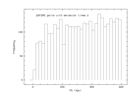
Figure 2: Histogram of the distribution of projected separations for the 3239 pairs in the 2dFGRS selected by : i) redshifts from emission lines and greater than 0.001, ii) angular separation less than 10′. The concordance model is assumed.

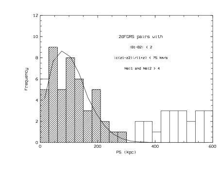
Figure 3: Selection of the sub-sample of interactivated galaxies candidates in the 2dFGRS. The zone of the 45 retained pairs with $PS<300\ (0.7/h_{\circ})$ kpc is hashed. The white case in the first bin is for the rejected pair in the arms of NGC 4517. The solid line displays the Poissonian distribution used for simulations.

The Multi-Object-Spectroscopy (MOS) with addressable fibres may induce a selection bias against close pairs through the mechanical width of “buttons” that attach fibres on the field plate, practically 33″ for the 2dF spectrograph. This drawback may be compensated for by a pertinent redundance of exposures. That bias may be evaluated (Mathew Colless, priv. com) when comparing photometric and spectroscopic catalogues of the 2dF. This inspection showed that the distribution of the number of pairs in angular separations are related well in the two catalogues above, as the number of pairs in the photometric catalogue are 30 % higher than in the spectroscopic one. That works, except for pairs closer than 18″ for which the ratio is higher. As there are only three such close pairs in our selected sample, we may estimate that this does not induce a noticeable bias in our estimated distribution of projected separations.

We then chose to extract the parameters of the distribution of $PS$ for interactivated galaxies from the sub-sample of 45 pairs with $PS<300(0.7/h_{\circ})$ kpc. Absolute magnitudes of the 90 objects range from -15.1 to -20.7 with -19.2 for the magnitude of mean luminosity and redshifts from 0.009 to 0.108 with a mean of 0.052. We fitted the histogram of $PS$ in Fig. 3 with a Poissonian probability law (a first attempt with a lognormal law was less satisfactory). The mean – and variance – of the Poissonian fitting is $105.3\ (0.7/h_{\circ})$ kpc .

We do not claim here to achieve a real measurement of the distribution of the projected separations of local interactivating galaxies: in the best case we got an estimation (presumably a majorant) of the relative dispersion of the $PS$. And there lies all we need to qualify the method. We note that the precise parameters of the real population will be updated on a larger sample with incoming data by the statistical study of the low redshift pairs that are spectroscopically confirmed.

At least, we tried to evaluate the orbital parameters of such encounters. A simple modeling with a Keplerian orbit between the first and second approaches and with an evolution of the SFR that is similar to that of Springel & Hernquist (Spri05 (2005)) seems to favour massive galaxies ($M_{1}+M_{2}\sim 10^{12}$ M_⊙) for the selected population. Fitting both the observed distribution of separations and that of relative radial velocities $\Delta v_{r}$ would indicate longer ($\times 2$ to $\times 3$) starbursts.

As explained above, we use that distribution of local projected separations to generate the synthetic samples, which includes the hypothesis that the statistical properties of the geometrical parameters of interactivations are independent of cosmic time. Reliance on that assumption is theoretically based on the consideration that the primum movens of both the interactivation – starburst – process and real separations is the – a priori constant – gravitational interaction. It is also founded on the fact that the $\sim 2.5\ 10^{5}$ 2dFGRS galaxies, from which our sample has been selected, have a wide dynamic of individual characteristics like masses and gas fractions. Then a statistical evolution of the characteristics of individual galaxies with redshift could have no first order effect on the linear separations of scarce interactivated pairs. The selection of primary interactivations is also an asset: those pairs are preferably constituted with gas-rich galaxies which are still quite free of strong merger experience. At any rate, numerical simulations would be the best way of quantifying how sensitive the distribution of separations is to parameters like mass, gas fraction, and gas properties of galaxies and then to estimate – and possibly correct – a redshift dependence.

3 Synthetic samples

3.1 Distribution in orientation

If $i$ is the inclination of the pair on the line of sight, the real linear separation $LS$ is related to the projected separation $PS$ by $LS=PS/\sin i$. If $i$ is not an easily observed parameter, the natural hypothesis for an isotropic distribution of pair orientation makes the set of possible directions homeomorphic to a Euclidean 2-sphere, and a simple integration on that sphere supplies the mean values: $<i>=1$ rad and $<\sin i>=\pi/4$. It is worth noting the latter value ($\sim 0.8$) of this projection factor, since it will explain why the unavailability of $i$ in the observations will not add a strong dispersion.

3.2 Distribution in linear separation

The expectation of the product of two independent random variables is the product of their expectations. Then the distribution of linear separations for the pairs of interactivated galaxies would have an expectation $105.3\ /\ (\pi/4)=134.1\ (0,7/h_{\circ})$ kpc.

There are two reasons for the dispersion of $PS$: linear separations and random orientations. The latter dispersion is that of $\sin i$. It has a standard deviation $\sigma\sim 0.22$ or a “relative dispersion” (standard deviation to mean ratio) of $\sim 0.22/(\pi/4)\approx 0.28$. That of the $PS$ of the 45 pairs extracted from the 2dFGRS is much greater : $72/109\approx 0.66$. Then the dispersion of the real sample is mainly due to the physical dispersion of linear separations, and the random inclination does not greatly affect the potentiality of the method.

We generated the linear separations in the mock samples of interactivated galaxies as a Poissonian distribution with expectation $134.1\ (0,7/h_{\circ})$ kpc before applying the projection effect of random orientation (previous subsection).

3.3 Distribution in redshift

The parentage between nuclear starbursts and true active nuclei, the similarity in their observing techniques, and the lack of deep samples of interactivated galaxies, all made it seems natural to use the distribution of redshift for a homogeneous sample of quasars.

Figure 4: Redshifts of QSOs in the 2QZ survey. We selected the 22 122 objects with only the label “QSO ”. This distribution of redshifts has been applied to the synthetic samples of interactivating galaxies

We chose the two-degree Field QSO redshift survey (2QZ) (Croom et al. Croom04 (2004)) in which we selected those 22 122 objects with the label “QSO ”. The histogram of redshifts is displayed in Fig. 4. In our synthetic process each pair then received a random redshift from that data base. All the random numbers and distributions above were generated with subroutines imported from “Numerical Recipes in Fortran” (imported from Press et al. Pre92 (1992)).

3.4 Distribution in $\Omega_{i\circ}$

With the purpose of estimating the inhomogeneity in the sensitivity of the method through the credible part of the $\Omega_{i\circ}$ field, we applied the whole procedure to a small set of tentative couples $(\Omega_{m\circ},\ \Omega_{\Lambda\circ}$). Then mock samples of ($\theta_{\circ}$, $z$) were generated through the Monte-Carlo method described above and with the general cosmological relations reviewed in Sect. 1.

4 Retrieving $\Omega_{i\circ}$

Retrieving $\Omega_{m\circ}$ and $\Omega_{\Lambda\circ}$ from the synthetic samples was solved by the Levenberg-Marquardt (LM) technique (routines in “Numerical Recipes”) which seemed well-suited to the non-linear and entangled inverse problem.

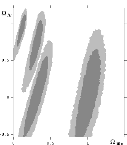
Figure 5: Normalized probability densities of retrieved cosmological parameters with 1000 pairs of interactivated galaxies. The 68% and 95% confidence levels appear in shaded and darker shaded areas for the four sets of ($\Omega_{m\circ}$, $\Omega_{\Lambda\circ}$): (1.0, 0.0), (0.3, 0.0), (0.3, 0.7), and (0.1, 0.9).

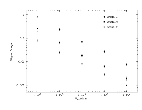
Figure 6: Internal precision ($\sigma$) on $\Omega_{m\circ}$ and $\Omega_{\Lambda\circ}$ versus number of pairs and for the “concordance” model, also shown with $\Omega_{f\circ}$ the precision with the flat space external condition $\Omega_{m\circ}+\Omega_{\Lambda\circ}=1$.

Figure  5 displays the potentiality of the method through the plausible zone of the ($\Omega_{m\circ},\ \Omega_{\Lambda\circ}$) field and only for 1000 pairs. We chose these four combinations:
(1.0, 0.0), (0.3, 0.0), (0.3, 0.7) and (0.1, 0.9). We assumed that all redshifts were known precisely. We checked the inversibility by applying that method to samples generated with zero dispersion in linear projected separations.

We summarise in Fig. 6 the standard deviations on $\Omega_{m\circ}$ and $\Omega_{\Lambda\circ}$ resulting from simulations ranging from $10^{2}$ to $10^{6}$ pairs. If an external condition is added to the sum $\Omega_{m\circ}+\Omega_{\Lambda\circ}$ (as with CMBR), the accuracy of the method is obviously enhanced. The standard deviations $\sigma_{i}$ of the fitted parameters all display a nominal decrease: $\sigma_{i}\propto 1/\sqrt{N\_pairs}$. As a matter of fact those accuracies are only internal to the method.

5 Observational prospects

5.1 Foreseeable data

As a surface of constant cosmic time of emisson $t_{e}$ is isometric to a Euclidean 2-sphere of radius $R(t_{e})r$, the elementary volume in a 1-steradian pencil and for sources emitting in the cosmic time interval $dt_{e}$ (thickness $dl$) is

$$dV=d_{A}^{2}\ dl=d_{A}^{2}\ c\ dt_{e}\ .$$ (8)

If $n(z_{c})$ is the density at redshift $z_{c}$, the number of sources per steradian in the range $\left[z_{c},z_{c}+dz_{c}\right]$ may be expressed as:

$$dN=n(z_{c})\ d_{A}^{2}\frac{c}{H(z_{c})(1+z_{c})}\ dz_{c}\ .$$ (9)

FL equations lead to

$$\frac{H}{H_{\circ}}=\left[\Omega_{m\circ}(1+z_{c})^{3}+1-\Omega_{m\circ}\right]^{{1\over 2}}$$ (10)

for a flat $\Lambda$CDM universe. Assuming $n(z_{c})=f_{\circ}(1+z_{c})^{m}$ ($m=3$ for a constant comoving density of sources), the total number of sources per steradian in the interval $\left[z_{c1},z_{c2}\right]$ may be deduced:

$$\begin{array}[]{l}\displaystyle{{N}=f_{\circ}\frac{c^{3}}{H_{\circ}^{3}}\int_{z_{c1}}^{z_{c2}}}[\Omega_{m\circ}(1+x)^{3}+1-\Omega_{m\circ}]^{-{1\over 2}}\\ \ \ \ \ \ \ \ \ \ \ \ \ \ \ \ \ \ \ \ \ \ \ \ \ \ \ \ \ \ \ \ \ \ \ \ (1+x)^{(m-3)}\ F^{2}(x)\ dx\ .\end{array}$$ (11)

Our 45 candidates were found in the $\sim 1500^{\tiny\squareforqed}$ (square degrees) field of the 2dFGRS. With a redshift interval $[0.001,0.108]$ and $m=3$, the local fequency is $f_{\circ}\sim 9400\ h^{3}\ {\mathrm{Gpc}^{-3}}$. For $h=0.7$ we get $f_{\circ}\sim 3000\ {\mathrm{Gpc}^{-3}}$.

We may evaluate the number of interactivated galaxies in a survey limited at $z_{l}\sim 3$. For the “concordance” model and $m=3$ we deduce a number of 80 interactivated pairs by square degree ($\sim 80^{{\tiny\ \squareforqed}^{-1}}$).

In fact it is presumable that the comoving density of interactivated pairs does increase with redshift, i.e. that the local real density $n(z_{c})$ increases more steeply than $(1+z_{c})^{3}$, leading to an underestimation of $n$. Le Fèvre & al (Lefev00 (2000)) derive a merger fraction of galaxies increasing as $\propto(1+z_{c})^{m}$ with $m={3.2\pm 0.6}$. Lavery & al. (Lav04 (2004)) deduce from collisional ring galaxies in HST deep field a galaxy interaction/merger rate with $m={5.2\pm 0.7}$ or even steeper. With $m=5$, the number of expected pairs by square degree up to $z_{c}=3$ climbs to $\sim 700^{{\tiny\ \squareforqed}^{-1}}$, a comfortable density for MOS. A $12^{{\tiny\ \squareforqed}}$ survey would then supply 1 000 interactivated pairs, if $m=3$. Some 10 000 pairs would be a foreseeable target in $100^{{\tiny\ \squareforqed}}$ and the total number of interactivated galaxies in a whole sky survey could be more than $10^{7}$ if $m>4$.

5.2 Inhomogeneities

Our universe is no longer the realisation of an FL model. The presence of inhomogeneities modifies the $\theta_{\circ}\longleftrightarrow z_{c}$ relation. This problem is difficult to solve mathematically. It was investigated long ago (Dashveski & Zeldovich Zeldo65 (1965), Dyer & Roeder Dyer72 (1972)). Hadrović & Binney (Hadro97 (1997)) used the methods of gravitational lensing to measure the involved biases. They derived a bias of $-0.17\pm 0.4$ on $q_{\circ}$, and showed that larger objects yield to smaller errors. Demianski et al. (Demia03 (2003)) derive exact solutions of $\theta_{\circ}(z)$ for some cases of locally inhomogeneous universes with a nonzero cosmological constant and approximate solutions for $z<10$. We note from those previous works that the size of our standard of length ($\sim 100$ kpc) would make our method less sensitive to inhomogeneities than would parsec size ultra-compact radio sources.

We also note that carrying out our method on real pairs of interactivated galaxies presupposes acquiring a wide-field imaging of those objects and then detecting all the possibly intervening galaxies or clusters close to the lines of sight. It would then be easy to exclude the most perturbed lines of sight and to limit the sample to regular directions of intervening space.

5.3 Observing

Interactivated galaxies with a mean projected separation above 100 kpc have (Sect. 3) a mean angular separation $\theta_{\circ}>10\arcsec$ over the whole range of $z$, and then the measure of $\theta_{\circ}$ will not add a significant dispersion in the data (the main dispersion remaining that of linear separation). The accuracy of measuring redshift $z$ is not a problem for those strong emission-line objects even with low dispersion spectroscopy (always compared to the intrinsic dispersion in the $\theta_{\circ}$ dimension).

The selection of primary interactivating pairs of galaxies seems achievable by wide-field imaging. Candidates may be selected by colours, magnitudes, angular separations, and morphology: the first approach of the two partners generally preserves a much simpler geometry for both of them than does the pre-merging second perigalacticon. Then a long or multi-slit spectrography with low dispersion (and low signal-to-noise ratio) would be enough to characterise and classify the starbursts and measure the redshifts. Integral field spectroscopy could be used – via its potentiality to supply velocity fields – to implement the classification criteria.

The main difficulty in running this program is obviously the faintness of those sources meant for spectroscopy with today’s telescopes. Without K-correction or extinction the distance modulus is supplied by the “luminosity distance” $d_{L}=d(1+z)$ (Mineur Min33 (1933), Robertson, Robert38 (1938)): $m-M=-5+5\log d_{L}$. The brightest members of the 45 2dFGRS pairs used in our ”real sample” would reach $V=26$ if located at $z=3$ in a concordance model (and close to $V=28$ for the mean of luminosities). But if we look at the distribution of 2dFQRS redshifts, only 21% have $z>2.$ and 4% $z>2.5$. The bulk of objects is centred on $z=1.6$, for which the V magnitudes would be 24.6 for the brightest ones and 26 for the mean of luminosity. The rejection (at any $z$) of less luminous objects could be an operational criterion.

If K-correction and – mainly intrinsic – extinction increase the above estimations, those two effects presumably are over-compensated by the increase of the intensities of starbursts with redshift: more gas in galaxies at remote times and the Schmidt law (Schmidt, Schmi59 (1959)) linking SFR to the the density of gas. As a matter of fact and even if they are mainly concerned with the “secondary” – pre-merger – starburst, many approaches in several wavelength ranges (see e. g. Mihos & Hernquist, Mihos94 (1994), Steidel & al, Steid99 (1999), Elbaz, Elbaz04 (2004)) measure a rapid increase of a factor $\sim 10$ (even without extinction correction) in the general SFR when looking backward in time from $z=0$ to $z\approx 1$ followed by a quasi-constant rate up to $z>3$.

Restricting the selection of candidates to balanced pairs – e.g. $\left|B_{1}-B_{2}\right|<1$ – could also be a means to favour strong starbursts. Another fact could help build feasibility in the future: due to its observational selection the 2QZ survey is, as already mentioned, very poor in $2<z<3$ objects and concentrated around $z\approx 1.5\pm 0.7$. In the real samples of interactivated galaxies, we may expect a distribution of redshifts that is less vanishing. Present uncertainties on that evolution mean that we do not try to further compute the foreseeable distribution in $z$ of a real sample of interactivated galaxies, but we do note that, in conjunction with the increase of starbursts luminosities with $z$, a high value of $m$ index or a distribution of $z$ simply that is flatter than for 2QZ would make the $\theta_{\circ}\longleftrightarrow z_{c}$ relation more sensitive to cosmological parameters, peculiar to $\Omega_{\Lambda\circ}$, but with the drawback of an increase in the fraction of faint high z objects.

With the foreseeable progress in the interactivation models, classifying diagnostics could be deduced. In each class the dispersion in linear (and projected) separations is expected to be lower, and each sub-sample could supply independent estimations of $\Omega_{i\circ}$ thereby giving both a test and more accuracy.

Finally the method could perhaps be applied to much brighter objects like interactivated pairs of Seyferts, if it could be established that they also have a characteristic distance distribution.

6 Conclusion

We studied a new method of observational cosmology using the angular size versus redshift relation and “primary interactivation” of pairs of galaxies as a natural generator of yardsticks. The properties of the population was estimated from the 2dFGRS. The number of those interactivated sources in the observable universe is much more than needed. Monte Carlo simulations show that an accuracy of $\pm 0.1$ on $\Omega_{m\circ}$ and $\Omega_{\Lambda\circ}$ seems feasible with a $\sim 10^{\tiny\squareforqed}$ survey. Reaching $\pm 0.01$ would imply a much wider survey and additional tests against bias. The method could also be used for constraining other free parameters of non-vacuum dark energy, quintessence, or other modified FL cosmologies. The main problem seems to be the faintness of remote sources for spectroscopy with today’s optical telescopes.